Geometric and Material Variability of the Probability of Landward Slope Failure for Homogeneous River Levees

Abstract

Holistic flood risk management (FRM) aims at minimizing the flood risk (FR) for an entire river basin. To this end, the probability of flooding and its consequences must also be taken into account in the planning of flood risk management measures. If the FR is to be limited by the flooding probability value (e.g., by changing the structural reliability), knowledge of the variability of the limit state is required. As an example, this study quantifies for the first time the variability of the probability of a landside slope failure on homogeneous river levees, using the Monte Carlo simulation. In the slip circle method developed by Krey that is used for this purpose, four geometric and six material input parameters are included as being uncertain, of which four emerge in the result as being relevant influencing variables of the failure probability. These analyses extend our understanding of landward slope failure by the variability of the limit state; the results allow a targeted adjustment of the local failure probability to limit the flood risk. In the future, the methodology presented is to be supplemented by the integration of parameter dependencies and, once in use, expanded to include structured cross-sections or additional failure mechanisms.

1. Introduction

Holistic flood risk management (FRM) aims at achieving a global minimum of flood risk (FR) in a river basin. Quantifying flood risk (FR) requires a comprehensive understanding of river basin processes, the genesis of floods, the behavior of flood protection systems, and the interaction of floods with floodplains. Therefore, and in light of global climatic changes, the aforementioned aspects have become the focus of current scientific work. Thus, AI-based methods for rainfall-runoff modeling [1] and advanced methods for remote sensing [2,3] are being developed, the regionality of flood events is being analyzed [4] and the behavior of the structural components of an FRM system is being described using advanced methods [5,6,7]. In addition, attempts are being made to transfer the vulnerability of floodplains into damage functions and, thus, to feed them into flood risk assessment [8,9].

$$FR=P\left(E\right)·C\left(E\right).$$

(1)

The FR is calculated according to Equation (1) from the product of the probability of occurrence, P, of an undesirable event, E, and the monetized consequences, C, that are associated with the event [10]:

In the context of this work, the unplanned flooding of a flood protection area as a result of structural failure is understood as one such undesirable event. Various failure mechanisms can cause such an event (e.g., overflow, slope failure, piping, or heave), even though this study is limited to the landside slope failure of a homogeneous river levee. While further failure mechanisms can be found elsewhere, e.g., in CIRIA [11] and ENW [12], the analyses of their probabilities can be taken from the works of Kortenhaus [13], Heyer [14] or Özer et al. [15].

The consequences of unplanned flooding depend, on the one hand, on the respective failure mechanism and, on the other hand, on the water level within the protected area. With hydraulic conditions assumed to be stationary for the purposes of this study, combined with the assumption that a levee breach inevitably results in the flooding of the protected area behind it, the consequences are simplified into a constant. As a result, the flood risk for this study can be described according to Equation (2):

$$FR=P_f·C \left(\mathrm{EUR}\right).$$

(2)

$P\left(E\right)$ or $P_f$ cannot be reduced to zero; in other words, there is always one FR that remains [16,17], and the public funds for the FRM are limited. Therefore, there is a need for a benefit-cost assessment in connection with the planning of FRM measures. For this reason, in Germany, there is a general principle of economic efficiency in the applicable regulations [18]. The key question of holistic FRM is, therefore: How can the risk associated with flood events be minimized using the available means?

On the one hand, a targeted industrial and settlement policy offers the possibility of influencing the consequences and, as a result, the FR [19]. On the other hand, the probability of flooding can be influenced. From a hydraulic point of view, upstream, downstream, and on-site measures are available for this purpose [12]. For example, runoff can be retained in the upper reaches of a river, so that the associated retention of the flood wave leads to a reduction in the flood peak at the reference site [16,20,21]. Regarding undercurrent, the discharge capacity can be increased, for example, by shortening flow paths or removing bottlenecks, which also results in a water level reduction at the reference site [22,23]. Finally, protective structures (such as river levees) can be built to prevent the flooding of a protected area [11].

If decision-makers define an acceptable flood risk ${\mathit{FR}}_{\mathit{req}}$ to be economically safeguarded, according to Equation (3), higher, acceptable probabilities of failure, $P_{f,\mathit{req},}$ will be the result for less vulnerable areas (small values for C) than for intensively used or highly vulnerable areas.

$$P_{f,req}=\frac{F{R}_{req}}{C} (-)$$

(3)

As a result, during a flood event, the hydraulic system tends to be relieved in less critical areas, i.e., the failure and flooding of a protected area, thus minimizing C for the benefit of the entire catchment area. To ensure the effectiveness of this approach, the over-dimensioning of protective structures (e.g., river levees) must be avoided. If, contrary to expectations, they should hold up in the case of a hydraulic event with a very low probability of occurrence, this increases the runoff and, thus, the risk of undercurrent. Therefore, knowledge of $P_f$ and its variability are essential when planning FRM measures.

The subject of this article is the variability of failure probability, using as an example the landside slope failure at homogeneous levee cross-sections. The variability is analyzed as a result of both geometrical and material input parameters. Therefore, this article begins with explaining the methodology of the study, then details the setup of the empirical experiment and the results, moving on to a discussion of the findings and, finally, our conclusions and outlook.

2. Methodology

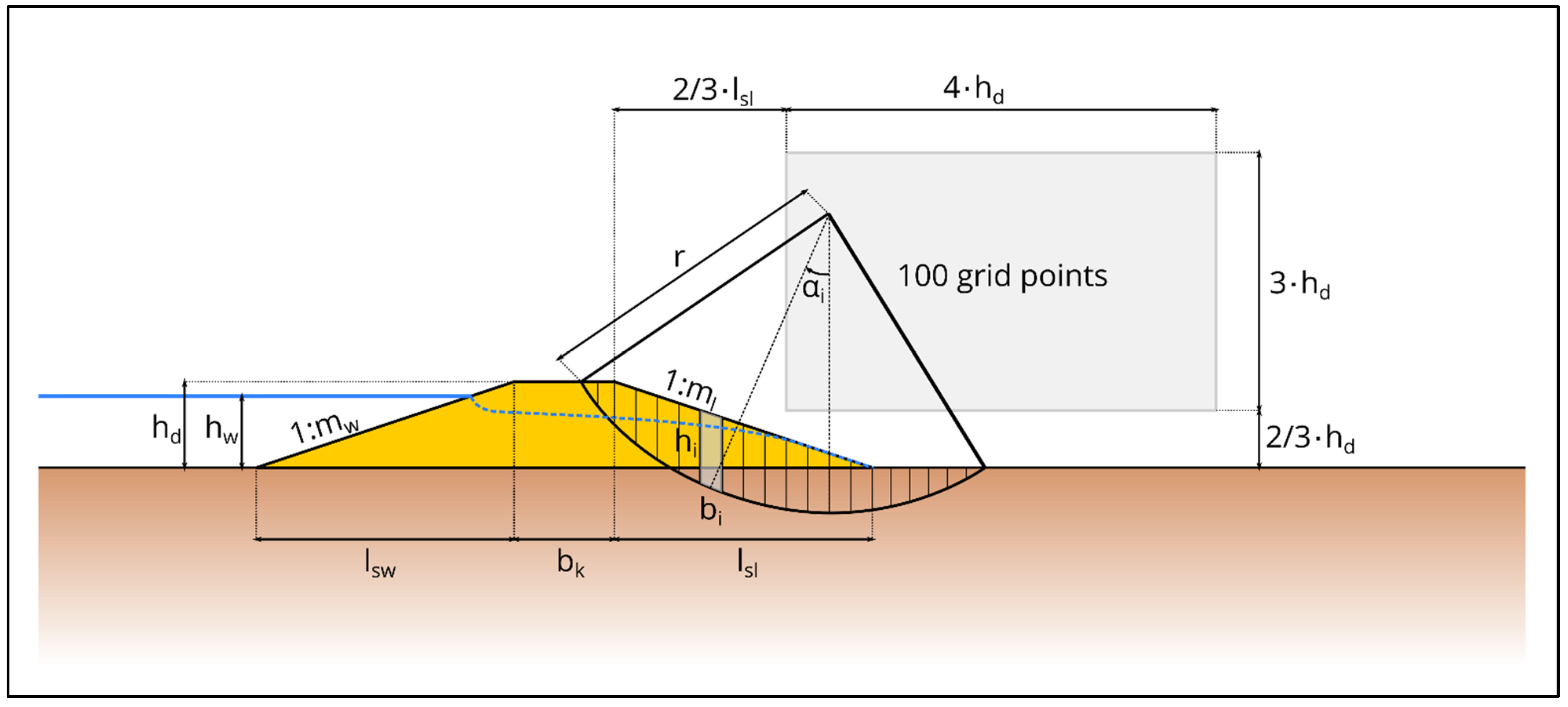
2.1. Levee Slope Stability

Levee failures occur repeatedly in connection with flood events and, in terms of a central levee failure database (ILPD) [24], failures can be categorized (e.g., according to the type of failure mechanism, return period of the hydraulic load, or geographical location) [15]. In practice, this results in a failure rate depending on the respective category, which can provide general indications of potentially critical areas [25]. The analysis of individual failure cases helps to broaden our understanding of the process leading to failure [7] and explains, for example, failures on cross-sections that were attested as being stable shortly before the event [6].

However, future-oriented flood risk management that adapts to climate change also requires enhanced forecasting methods, e.g., for risk-based design. While limit state analyses based on laboratory tests are only possible on a small scale [26] and finite element analyses, such as random-finite-element analyses [27], are computationally expensive, analytical methods, due to their simplicity, offer the possibility of running a large number of simulations in a short time, thus allowing less specific but very comprehensive studies.

With regard to the aforementioned ILPD, landward slope failure, both in the form of micro-stability (where sliding mass is limited to the levee cubature) and macro-stability (where sliding mass includes the subsoil (see also [24])) is one of the failure mechanisms most frequently observed on river levees [14,15]. Other failure mechanisms relevant to river levees are overflow and backward piping, initiated by suffusion and heave [15,28,29,30]. To calculate the slope stability analytically, the effects and the resistance of a sliding mass on an effective plane (sliding surface) are compared and, thus, the reliability against sliding is checked. While the calculation method developed by Janbu [31] determines the moment equilibrium of an entire sliding mass with a circular-cylindrical sliding surface, in the methods developed by Bishop [32], Krey [31], and Fellenius [33], this analysis takes place with many small sliding bodies (vertical lamellae). The lamella-based method according to Bishop corresponds to the state of the art in Germany [34]. This is an iterative procedure for which an initial value of stability must be assumed. Since the Krey method is based on the same sliding surface, it assesses the critical state ($S=R$) equally [31] and is not iterative; it has its advantages over the Bishop method in terms of the computing time required for implementation via numerical, probabilistic analyses. Consequently, this is the method used in the context of this work. Conventionally, the stability statement is made using the safety factor $\eta =R/S$ (cf. Equation (4) and Figure 1). In Equation (4), $T_i$ is the tangential force, and $G_i$ is the weight of the $i$-th lamella of width $b_i$ in the sliding surface, inclined at an angle, ${\alpha }_i,$ to the vertical. $\phi$ denotes the angle of friction and $c$ denotes the cohesion of the soil.

$$\eta =\frac{R}{S}=\frac{{{\displaystyle \sum }}_{i=1}^n{T}_i·r}{{{\displaystyle \sum }}_{i=1}^n{G}_i·r·\sin {\alpha }_i}=\frac{{{\displaystyle \sum }}_{i=1}^n\left(\frac{G_i·\tan \phi +c·b_i}{\sin {\alpha }_i·\tan \phi +\cos {\alpha }_i}\right)·r}{{{\displaystyle \sum }}_{i=1}^n{G}_i·r·\sin {\alpha }_i} (-)$$

(4)

For the analysis of the probability of failure (cf. Section 2.3), it is recommended to compare stress and resistance based on the reliability $z$ (cf. Equation (5)). Compared to the consideration of $\eta$, $z$ has procedural advantages, which are described in Section 2.3.

$$z=R-S={{\displaystyle \sum }}_{i=1}^n\left(\frac{G_i·\tan \phi +c·b_i}{\sin {\alpha }_i·\tan \phi +\cos {\alpha }_i}\right)·r-{{\displaystyle \sum }}_{i=1}^n{G}_i·r·\sin {\alpha }_i (-)$$

(5)

The weight force $G_i$ is calculated from the gravitational constant $g$, the cross-sectional area of a lamella, $A_i$, the moisture density of each soil, ${\rho }_{f,j,}$ and its percentage of the cross-sectional area. $p_{s,i,j}$.

$$G_i=g·A_i·{{\displaystyle \sum }}_{j=1}^m{\rho }_{f,j}·\frac{p_{s,i,j}}{100} (\mathrm{kN}/\mathrm{m})$$

(6)

The moisture density is determined in turn from the grain density, ${\rho }_g$, the porosity, $n,$ and the water content, $w$.

$${\rho }_f=\left(1-n\right)·{\rho }_g·\left(1+w\right) (\mathrm{kg}/{\mathrm{m}}^3)$$

(7)

2.2. Probabilistic Input Parameters

To determine the probability of failure, the availability of stochastic distributions of the input parameters is a mandatory requirement [35,36]. In the context of slope stability, the porosity, as the ratio of the pore volume to the sample volume ${n=V}_{\mathit{pore}}{/V}_{\mathit{sample}}$, the internal friction angle $\phi$, the cohesion $c$, the grain density ${\rho }_g,$ and the water content $w,$ are relevant variables. For frequently performed soil mechanical tests (e.g., sieve analysis, dynamic probing), there are collections of stochastic quantities, such as those found in Baecher and Christian [35] or ISSMGE-TC304 [37]. In a previous study, distributions of selected soil mechanical parameters were estimated by transforming the results from classification tests [38]. In combination with comprehensive literature research [13,31,39,40,41,42,43,44,45,46,47,48,49], as well as on experience from the development of the calculation program used [50,51], this study is based on the distributions given in

Table 1. Distribution type (distribution), the expected value (E), and coefficient of variation (COV) of the friction angle $\phi$, the cohesion $c$ and the porosity $n$ for 13 soil types, classified according to the German regulations (DIN 18196). The data entries used in the reference levee system are highlighted in grey (literature resources: [13,31,39,40,41,42,43,44,45,46,47,48,49]).

Soil Types	$\mathbf{Friction}\mathbf{Angle}\mathbf{\phi }$			$\mathbf{Cohesion}\mathit{c}$			$\mathbf{Porosity}\mathit{n}$
	Distribution	E [°]	COV [−]	Distribution	E [kN/m²]	COV [−]	Distribution	E [−]	COV [−]
GE	Normal	36.4	0:1	Lognormal	0	0.3	Normal	0.30	0.2
GW, GI		36.9			0
GU, GT		38			3.5
GU*, GT*		35.5			10
SE		35.3			0			0.40
SW, SI		35.5			0
SU, ST		34.5			3
SU*, ST*		32			9.3
UL		30.1	0.3		5.6			0.50
UM, UA		27.9			8.4
TL		26.9			15.6
TM		24.3			20
TA		21.6			23.1

.

Due to the generally small variability of grain density [52] and the sparse availability of water content distribution, the same invariant input distributions are used for both soils considered in this study. Accordingly, a normal distribution, with an expected value of $\mathrm{E}=2.650\frac{\mathrm{kg}}{{\mathrm{m}}^3}$ and a coefficient of variation of $\mathrm{COV}=10\%,$ is considered for ${\rho }_g,$ and $\mathrm{w}$ enters the analyses using an exponential distribution with $\mathrm{E}=0.075$ and $\mathrm{COV}=30\%$, in accordance with the recommendations of Bachmann et al. [51].

2.3. Determination of Failure Probability

In terms of the analysis of slope stability, failure is a condition wherein the stress exceeds the resistance $\left(S>R\right)$. If the resistance is greater than the stress ($S<R$), there is a state of non-failure, which in engineering practice is referred to as “stable”. If the stress and resistance are equal ($S=R$), the limit state is present. According to Equation (5), failure occurs when $z$ is less than zero. The probability of failure can, therefore, be determined by integrating the density function of the reliability $f\left(z\right)$ over the negative range of values (cf. Equation (8)).

$$P_f=P\left(z<0\right)={{\displaystyle \int }}_{-\infty }^{0}f\left(z\right)dz (-)$$

(8)

Due to the partly non-normally distributed input parameters (cf. Table 1) and the often non-linear limit state equations (cf. Equation (5)), $f_z\left(z\right)$ usually results in a complex density function, the integration of which is not trivially possible. However, in order to estimate $P_f$, both analytical (e.g., FOSM, FORM, SORM) and numerical methods, such as the Monte Carlo simulation (MCS), are available. An overview of analytical approximation methods can be found in, e.g., Baecher and Christian [35], Ang and Tang [36], and Schneider and Schlatter [53]. While Baecher and Christian [35] and the DWA Deutsche Vereinigung für Wasserwirtschaft, Abwasser und Abfall [54] give an introduction to Monte Carlo analysis, Möllmann [55] and Huber [56] provide additional optimization methods. The implementation of the MCS used in this study is subject to the open-source software ProMaIDes [50]. $P_f$ is approximated by the $n_{\mathrm{sim}}$-fold repetition of the stability analysis with scattering input parameters according to their distribution. At the same time, the number of parameter combinations leading to failure is recorded in a counter variable, $n_f$. The approximate failure probability, $P_{f,\mathrm{MCS}},$ is thus obtained according to Equation (10) for the realized simulation number, $n_p$.

$$\underset{n_{sim}\to \infty }{\lim }{P}_{f,MCS}=P_f=\frac{n_f}{n_{sim}} (-)$$

(9)

$$\underset{n_{sim}\to n_p}{\lim }{P}_{f,MCS}\approx P_f=\frac{n_f}{n_p} (-)$$

(10)

$$n_p=\frac{10}{P_f} (-)$$

(11)

The larger the value of $n_p$, the more accurate the approximation of $P_f$. However, an increase in $n_p$ is accompanied by a longer calculation time, so it is common practice to choose an $n_p$ value an order of magnitude larger than the expected probability of failure. For an expected failure probability of the order of $P_f \approx 1 \times {10}^{-3}$, $n_p \ge 1 {\times 10}^4$, simulations must thus be carried out (cf. Equation (11)).

The probabilistic assessment of levee stability is usually carried out for defined river levee cross-sections with stochastically describable material properties. If either the geometric or the material input parameters are changeable, this applies equally to the stability assessment. This variability may be a consequence of epistemic uncertainties or of the more targeted influencing of input parameters in the context of planning FRM measures.

3. Setup of Empirical Experiment

To quantify the variability of a landward slope failure, stability analyses are conducted for the cross-section of a homogeneous reference levee on cohesive subsoil (see Figure 1) that is geared toward the minimum requirements in Germany [9]. The levee’s dimensions are: height ${\mathrm{h}}_{\mathrm{d}}=4.5 \mathrm{m}$, crown width ${\mathrm{b}}_{\mathrm{k}}=3.5 \mathrm{m},$ with both a water and landside slope inclination of ${\mathrm{m}}_{\mathrm{w}}{=\mathrm{m}}_{\mathrm{l}}=3$. Therefore, the reference levee has a cross-sectional area of $\mathrm{A}=76.5 {\mathrm{m}}^2$ and presents at a deterministic water level, ${\mathrm{h}}_{\mathrm{w}}=4.0 \mathrm{m}$, with the minimum freeboard ${\mathrm{f}}_{\min }=0.5 \mathrm{m}$.

The reference condition has a failure probability of $P_{f,\mathrm{ref}}$. During the analyses, this is modified geometrically and in terms of its material properties. To put these modifications into perspective, the modified parameter configuration $X_i\prime$ is compared with the reference state $X_i$ (see Equation (12)). The modified parameters are the four geometric input parameters (${\mathrm{h}}_{\mathrm{d}}$, ${\mathrm{b}}_{\mathrm{k}}$, ${\mathrm{m}}_{\mathrm{w}}$, ${\mathrm{m}}_{\mathrm{l}}$; see Figure 2), along with the expected value $\mathrm{E}$ and the coefficient of variation $\mathrm{COV}$ of the internal friction angle $\phi$, the cohesion $c,$ and the porosity $n$. The modifications are based on the experience intervals reported in the literature for both $\mathrm{E}$ and $\mathrm{COV}$, so that the investigation intervals of the material analysis are defined as $\left[0.7·{\mathrm{E}}_{\mathrm{rel}}{ < \mathrm{E}}_{\mathrm{rel}} < 1.3·{\mathrm{E}}_{\mathrm{rel}}\right]$ and $[0.3·{\mathrm{COV}}_{\mathrm{rel}}{ < \mathrm{COV}}_{\mathrm{rel}} < 5·{\mathrm{COV}}_{\mathrm{rel}}]$.

$$X_{i,rel}=\frac{X_i^{\prime }}{X_i} mit X_i=\left(\mathrm{A}, \mathrm{E}, \mathrm{COV}\right) (-)$$

(12)

Table 2. Study intervals of the geometric variables and the associated reference cross-sectional area.

Nr.	Variable Xi	Unit	$\mathbf{Bounds} \mathbf{of} \mathbf{the} \mathbf{Interval} \mathbf{of} {\mathit{X}}_{\mathit{i}}$		$\mathbf{Bounds} \mathbf{of} \mathbf{the} \mathbf{Interval} \mathbf{of} {\mathit{X}}_{\mathit{i},\mathit{r}\mathit{e}\mathit{l}}$
			Lower	Upper	Lower	Upper
1	${\mathrm{h}}_{\mathrm{D}}$	m	4.00	6.0	0.8	1.7
2	${\mathrm{b}}_{\mathrm{K}}$	m	0.10	8.0	0.8	1.2
3	${\mathrm{m}}_{\mathrm{w}}$	-	1.50	5	0.8	1.2
4	${\mathrm{m}}_{\mathrm{l}}$	-	1.50	5	0.8	1.2
5	$\mathrm{E}\left(\phi \right)$	°	24.2	44.9	0.7	1.3
6	$\mathrm{E}\left(c\right)$	kN/m²	2.1	5.1	0.7	1.3
7	$\mathrm{E}\left(n\right)$	-	0.3	0.5	0.7	1.3
8	$\mathrm{COV}\left(\phi \right)$	%	3.0	50.0	0.3	5.0
9	$\mathrm{COV}\left(c\right)$	%	9.0	150.0	0.3	5.0
10	$\mathrm{COV}\left(n\right)$	%	6.0	100.0	0.3	5.0

provides a summary of the studied intervals in both absolute and relative bounds. The comparison of the reference and the modified states results in discrete values for the influence of the investigated parameters. Using regression analysis, empirical functions according to Equation (13) are determined (see Appendix A).

$$P_f=f\left(X_{i,rel}\right) (-)$$

(13)

In addition, the variability of the expected value $\mathrm{E}$ and the coefficient of variation $\mathrm{COV}$ are integrated into the analyses. Based on a reference system with the material properties presented in Table 1, either $\mathrm{E}$ or $\mathrm{COV}$ for the aforementioned soil mechanical variables are changed to take account of material-related variability (see Table 2).

In practice, a special role is assigned to cohesion in the stability analyses, as its physical cause and ubiquitous effectiveness are discussed in the soil mechanics community, e.g., as found in Kolymbas [32] or Kempfert and Raithel [52]. Cohesion is taken into account by engineering conservative analyses, which partly neglect cohesion or only include it proportionally. In the context of this work, cohesion is taken under consideration by analyzing the scenarios defined in

Table 3. Consideration of cohesion in the individual scenarios; if “yes”, $c$ is considered as a random variable, if “no”, $\mathrm{E}\left(c\right)=0$ and $\mathrm{COV}\left(c\right)=0$.

Scenario	Cohesion
	Levee	Subsoil
1	No	No
2-1	Yes	No
2-2	No	Yes
3	Yes	Yes

.

4. Results

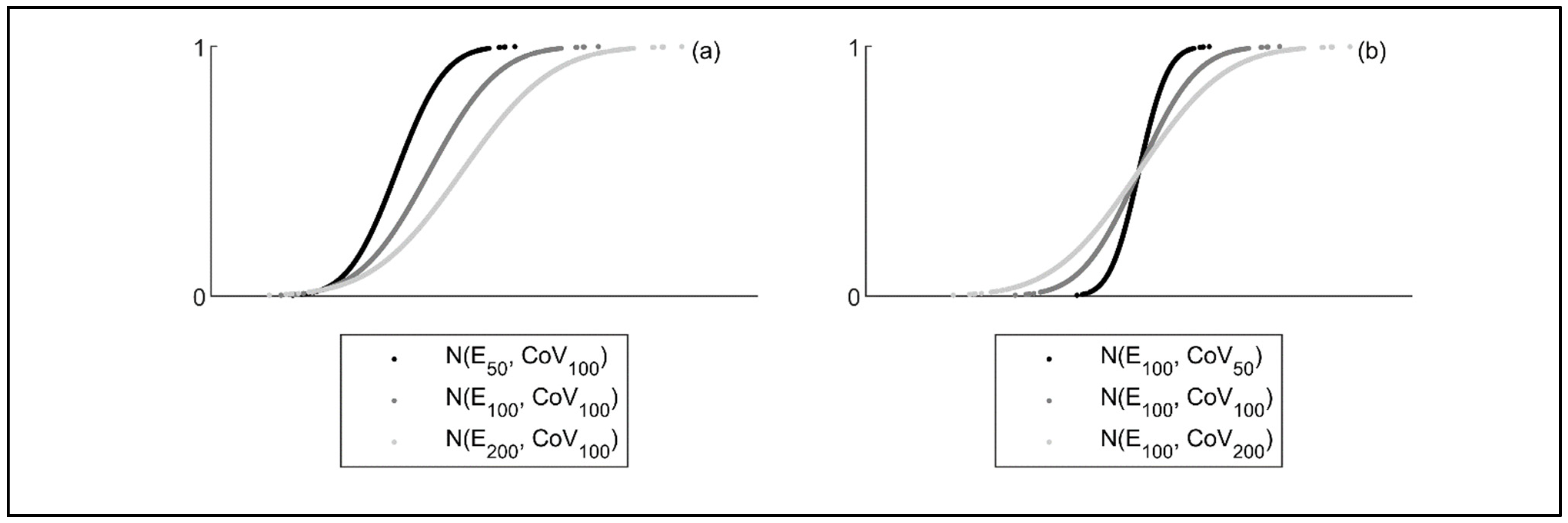
4.1. Variability Quantification

For the ten input parameters considered as variables according to Table 2, discrete function curves will result for each scenario in Table 3 with regard to Equation (13). This means that for eight of the parameters, there are four functions each and for the two analyses of cohesion, there are two functions each (cf. Figure 3). For the reference condition (abscissa value 1.0), the expected failure probability from Scenario 1 is 4.2 × 10⁻¹, which is over 600 times higher than for Scenario 3 with 6.8 × 10⁻⁴. This illustrates the relevance of the engineering approach to cohesion in terms of model definition.

The landward slope inclination, ${\mathrm{m}}_{\mathrm{l}}$, the expected value of the internal friction angle $\mathrm{E}\left(\phi \right)$, the coefficient of variation $\mathrm{COV}\left(\phi \right),$ and the expected value of porosity $\mathrm{E}\left(n\right)$ have an influence on the probability of a landward slope failure. For these four input parameters, the trends that are quantified by means of regression analysis can be found in the Appendix A (cf.

Table A1. Evaluation of the trends of the airside slope ${\mathrm{m}}_{\mathrm{l}}$ and the expected value, as well as the coefficient of variation of the friction angle $\mathrm{E}\left(\phi \right)$ and the expected value, as well as the coefficient of variation of porosity $\mathrm{E}\left(n\right)$.

Variable	Scenario	Model	Equation	Validity Interval	R2
${\mathrm{m}}_{\mathrm{l}}$	1	rational	$P_f=\frac{0.2974{\mathrm{A}}_{\mathrm{rel}}^2-0.7061{\mathrm{A}}_{\mathrm{rel}}+0.4279}{{\mathrm{A}}_{\mathrm{rel}}^2-1.833{\mathrm{A}}_{\mathrm{rel}}+0.8794}$	$0.8<{\mathrm{A}}_{\mathrm{rel}}<1.2$	0.9985
	2-1	rational	$P_f=\frac{-1139{\mathrm{A}}_{\mathrm{rel}}+1745}{{\mathrm{A}}_{\mathrm{rel}}^2+1.863·{10}^4{\mathrm{A}}_{\mathrm{rel}}-1.323·{10}^4}$	$0.8<{\mathrm{A}}_{\mathrm{rel}}<1.2$	0.9962
	2-2	rational	$P_f=\frac{-0.2286{\mathrm{A}}_{\mathrm{rel}}^3+0.907{\mathrm{A}}_{\mathrm{rel}}^2-1.185{\mathrm{A}}_{\mathrm{rel}}+0.5112{\mathrm{A}}_{\mathrm{rel}}}{{\mathrm{A}}_{\mathrm{rel}}^2-1.792{\mathrm{A}}_{\mathrm{rel}}+0.8205}$	$0.8<{\mathrm{A}}_{\mathrm{rel}}<1.2$	0.9970
	3	exponential	$P_f=6.319·{10}^{10}{\mathrm{e}}^{-35.89{\mathrm{A}}_{\mathrm{rel}}}+1.822·{10}^{-4}{\mathrm{e}}^{0.7624{\mathrm{A}}_{\mathrm{rel}}}$	$0.8<{\mathrm{A}}_{\mathrm{rel}}<1.2$	0.9807
$\mathrm{E}\left(\phi \right)$	1	rational	$P_f=\frac{0.09514{\mathrm{E}}_{\mathrm{rel}}{\left(\phi \right)}^2-0.1209{\mathrm{E}}_{\mathrm{rel}}\left(\phi \right)+0.04229}{{\mathrm{E}}_{\mathrm{rel}}{\left(\phi \right)}^3-2.087{\mathrm{E}}_{\mathrm{rel}}{\left(\phi \right)}^2+1.472{\mathrm{E}}_{\mathrm{rel}}\left(\phi \right)-0.3463}$	$0.7<{\mathrm{E}}_{\mathrm{rel}}\left(\phi \right)<1.3$	0.9998
	2-1	rational	$P_f=\frac{0.07275{\mathrm{E}}_{\mathrm{rel}}{\left(\phi \right)}^2-0.1738{\mathrm{E}}_{\mathrm{rel}}\left(\phi \right)+0.1895}{{\mathrm{E}}_{\mathrm{rel}}\left(\phi \right)-0.1557}$	$0.7<{\mathrm{E}}_{\mathrm{rel}}\left(\phi \right)<1.3$	0.9996
	2-2	rational	$P_f=\frac{0.153{\mathrm{E}}_{\mathrm{rel}}{\left(\phi \right)}^2-0.4036{\mathrm{E}}_{\mathrm{rel}}\left(\phi \right)+0.2674}{{\mathrm{E}}_{\mathrm{rel}}{\left(\phi \right)}^2-1.562{\mathrm{E}}_{\mathrm{rel}}\left(\phi \right)+0.665}$	$0.7<{\mathrm{E}}_{\mathrm{rel}}\left(\phi \right)<1.3$	0.9998
	3	exponential	$P_f=27.51{\mathrm{e}}^{-14.86{\mathrm{E}}_{\mathrm{rel}}\left(\phi \right)}+7.548·{10}^{-4}{\mathrm{e}}^{-0.1102{\mathrm{E}}_{\mathrm{rel}}\left(\phi \right)}$	$0.7<{\mathrm{E}}_{\mathrm{rel}}\left(\phi \right)<1.3$	0.9852
$\mathrm{E}\left(n\right)$	1	linear	$P_f=0.5566{\mathrm{E}}_{\mathrm{rel}}\left(n\right)-0.1115$	$0.7<{\mathrm{E}}_{\mathrm{rel}}\left(n\right)<1.3$	0.9855
	2-1	polynomial	$P_f=0.03047{\mathrm{E}}_{\mathrm{rel}}{\left(n\right)}^2-0.06989{\mathrm{E}}_{\mathrm{rel}}\left(n\right)+0.1437$	$0.7<{\mathrm{E}}_{\mathrm{rel}}\left(n\right)<1.3$	0.9804
	2-2	linear	$P_f=0.5678{\mathrm{E}}_{\mathrm{rel}}\left(n\right)-0.3834$	$0.7<{\mathrm{E}}_{\mathrm{rel}}\left(n\right)<1.3$	0.9675
	3	linear	$P_f=-1.26·{10}^{-3}{\mathrm{E}}_{\mathrm{rel}}\left(n\right)+2.003·{10}^{-3}$	$0.7<{\mathrm{E}}_{\mathrm{rel}}\left(n\right)<1.3$	0.9879
$\mathrm{CoV}\left(\phi \right)$	1	rational	$P_f=\frac{7.434·{10}^{-3}{\mathrm{CoV}}_{\mathrm{rel}}{\left(\phi \right)}^3+0.4776{\mathrm{CoV}}_{\mathrm{rel}}{\left(\phi \right)}^2-0.4388{\mathrm{CoV}}_{\mathrm{rel}}\left(\phi \right)+0.3401}{{\mathrm{CoV}}_{\mathrm{rel}}{\left(\phi \right)}^2-0.9612{\mathrm{CoV}}_{\mathrm{rel}}\left(\phi \right)+0.8566}$	$0.3<{\mathrm{CoV}}_{\mathrm{rel}}\left(\phi \right)<5$	0.9981
	2-1	rational	$P_f=\frac{0.1827{\mathrm{CoV}}_{\mathrm{rel}}{\left(\phi \right)}^2-0.8458{\mathrm{CoV}}_{\mathrm{rel}}\left(\phi \right)+2.53}{{\mathrm{CoV}}_{\mathrm{rel}}{\left(\phi \right)}^2-7.259{\mathrm{CoV}}_{\mathrm{rel}}\left(\phi \right)+24.16}$	$0.3<{\mathrm{CoV}}_{\mathrm{rel}}\left(\phi \right)<5$	0.9995
	2-2	rational	$P_f=\frac{0.4889{\mathrm{CoV}}_{\mathrm{rel}}{\left(\phi \right)}^2-0.2789{\mathrm{CoV}}_{\mathrm{rel}}\left(\phi \right)+0.1017}{{\mathrm{CoV}}_{\mathrm{rel}}{\left(\phi \right)}^2+0.4419{\mathrm{CoV}}_{\mathrm{rel}}\left(\phi \right)+0.4462}$	$0.3<{\mathrm{CoV}}_{\mathrm{rel}}\left(\phi \right)<5$	0.9996
	3	rational	$P_f=\frac{0.09995{\mathrm{CoV}}_{\mathrm{rel}}{\left(\phi \right)}^2-0.2471{\mathrm{CoV}}_{\mathrm{rel}}\left(\phi \right)+0.1435}{{\mathrm{CoV}}_{\mathrm{rel}}{\left(\phi \right)}^2-7.619{\mathrm{CoV}}_{\mathrm{rel}}\left(\phi \right)+25.52}$	$0.3<{\mathrm{CoV}}_{\mathrm{rel}}\left(\phi \right)<5$	0.9992
$\mathrm{CoV}\left(n\right)$	1	rational	$P_f=\frac{0.5572{\mathrm{CoV}}_{\mathrm{rel}}{\left(n\right)}^2-0.1406{\mathrm{CoV}}_{\mathrm{rel}}\left(n\right)+1.658}{{\mathrm{CoV}}_{\mathrm{rel}}{\left(n\right)}^2-0.1796{\mathrm{CoV}}_{\mathrm{rel}}\left(n\right)+4}$	$0.3<{\mathrm{CoV}}_{\mathrm{rel}}\left(n\right)<5$	0.9974
	2-1	rational	$P_f=\frac{0.1473{\mathrm{CoV}}_{\mathrm{rel}}{\left(n\right)}^2-0.9986{\mathrm{CoV}}_{\mathrm{rel}}\left(n\right)+3.094}{{\mathrm{CoV}}_{\mathrm{rel}}{\left(n\right)}^2-8.887{\mathrm{CoV}}_{\mathrm{rel}}\left(n\right)+29.41}$	$0.3<{\mathrm{CoV}}_{\mathrm{rel}}\left(n\right)<5$	0.9996
	2-2	rational	$P_f=\frac{0.4022{\mathrm{CoV}}_{\mathrm{rel}}{\left(n\right)}^2-0.1748{\mathrm{CoV}}_{\mathrm{rel}}\left(n\right)+0.8819}{{\mathrm{CoV}}_{\mathrm{rel}}{\left(n\right)}^2-0.6803{\mathrm{CoV}}_{\mathrm{rel}}\left(n\right)+6.501}$	$0.3<{\mathrm{CoV}}_{\mathrm{rel}}\left(n\right)<5$	0.9997
	3	rational	$P_f=\frac{5.954·{10}^{-3}{\mathrm{CoV}}_{\mathrm{rel}}{\left(n\right)}^3-1.624·{10}^{-3}{\mathrm{CoV}}_{\mathrm{rel}}{\left(n\right)}^2-1.655·{10}^{-3}{\mathrm{CoV}}_{\mathrm{rel}}\left(n\right)+0.01233}{{\mathrm{CoV}}_{\mathrm{rel}}{\left(n\right)}^2-7.861{\mathrm{CoV}}_{\mathrm{rel}}\left(n\right)+20.4}$	$0.3<{\mathrm{CoV}}_{\mathrm{rel}}\left(n\right)<5$	0.9995

). On the other hand, the results for the water-side slope ${\mathrm{m}}_{\mathrm{w}}$, the crown width ${\mathrm{b}}_{\mathrm{K}}$, and the expected value of the cohesion $\mathrm{E}\left(c\right),$ as well as the coefficients of variation of cohesion $\mathrm{COV}\left(c\right)$ and porosity $\mathrm{COV}\left(n\right),$ do not show any influences within the reported experience intervals. In light of the slip circle illustrated in Figure 1, it becomes clear that the water-side slope has no influence, and the crown width has only a small influence on the geometry of the sliding mass. With an expected value of 3 kN/m² and a coefficient of variation of 30 percent, the cohesive effect of the levee body is small, both in general and in comparison to that of the subsoil (cf. Table 1). The section modulus from Equation (5) is, therefore, largely determined by the properties of the subsoil, so that changes to the values of the cohesion in the levee body have no effect on the stability statement. Accordingly, macro stability prevails.

In detail, a negatively correlated trend can be seen for the landward slope ${\mathrm{m}}_{\mathrm{l}}$ in all scenarios. This means that the flatter the slope and the larger the relative cross-sectional area according to Equation (12) (cf. Figure 3), the smaller the probability of failure of the landside slope. In Scenarios 1 and 2-1, the reduction in failure probability is smaller than in Scenarios 2-2 and 3, with the smallest calculated failure probability associated with a value of 4.6 × 10⁻⁴ for Scenario 3 and a 20% increase in cross-sectional area (corresponding to a levee slope of ${\mathrm{m}}_{\mathrm{l}}=5$). The expected value of the friction angle $\mathrm{E}\left(\phi \right)$ also shows a negatively correlated trend and exhibits the greatest influence for scenarios with a cohesive substrate. The influence of the subsoil is also confirmed in the results on the coefficient of variation of the internal friction angle, $\mathrm{COV}\left(\phi \right)$. However, this shows a positively correlated trend, i.e., the more the internal friction angle scatters, the greater the expected probability of failure. In the context of the internal friction angle and within the considered value intervals, the probability of failure is reduced to 6.4 × 10⁻⁴ (in the case of $1.3·\mathrm{E}\left(\phi \right)=44.9°$) or else 6.8 × 10⁻⁴ (in the case of $0.3·\mathrm{VarK}\left(\phi \right)=3\%$).

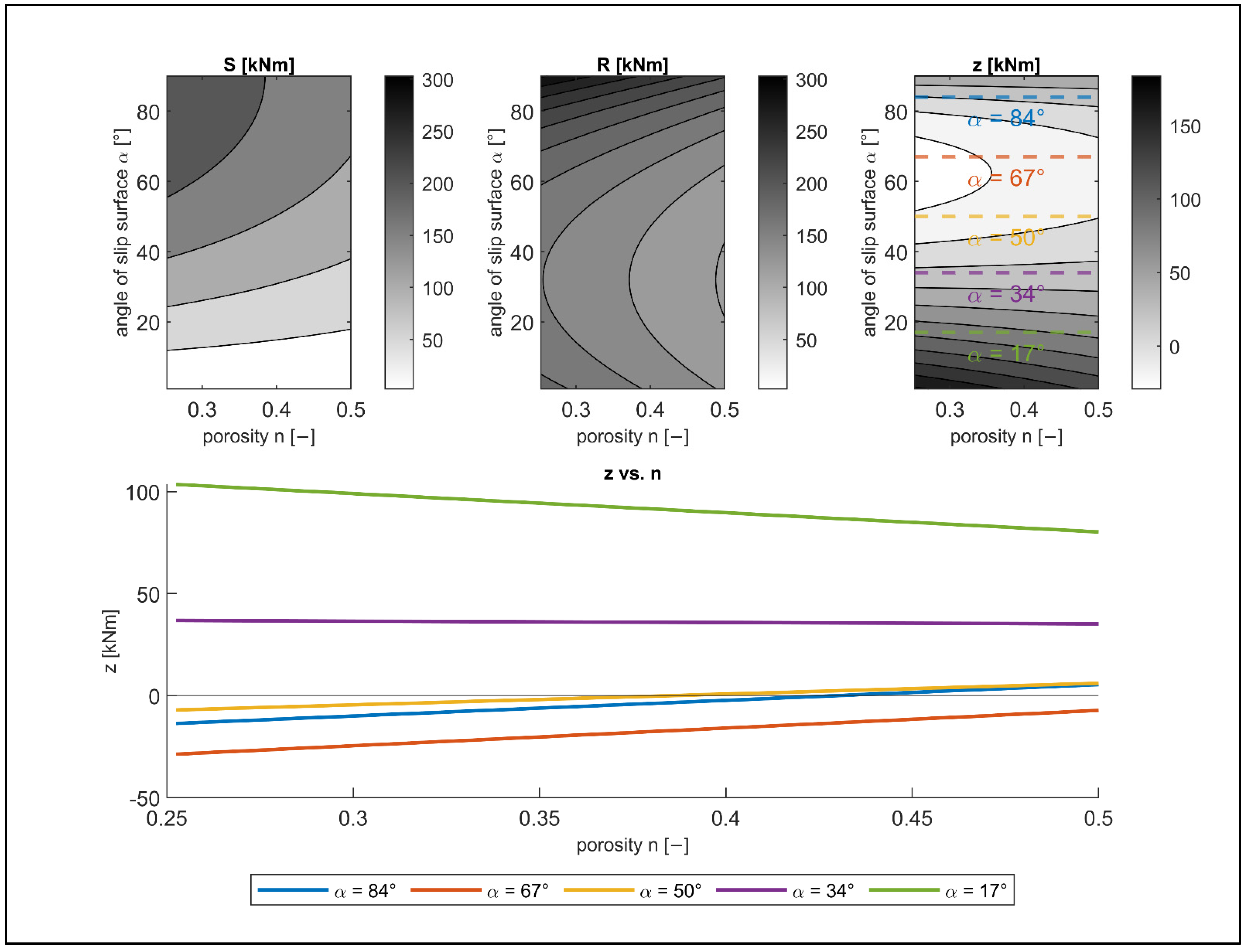
4.2. Influence of Porosity

It is striking that the results for the expected value of porosity $\mathrm{E}\left(n\right)$ show positively correlated trends for cohesionless levee cross-sections and no or negatively correlated trends for cohesive levee cross-sections. An increase in $\mathrm{E}\left(n\right)$ means an increase in the pore fraction of a defined soil volume. Since the pores are usually filled with either water or air, the increase in pores means a reduction in the average density and, in connection with gravity, also in the density of the soil. Consequently, as $\mathrm{E}\left(n\right)$ increases, the weight force of the floor lamella, $G_i,$ decreases. Now, according to Equation (5), $G_i$ has an influence on both the driving and the holding moments of the slip circle, so that the influence of the porosity is shown in the following using a deterministic interval calculation, for the sake of clarity.

If one considers a single lamella as a vertical column on a slip circle, the stress $S$ (driving moment), the resistance $R$ (holding moment) and the reliability $z$ can be determined for different positions of the lamella along the slip circle (cf. Figure 4). If the porosity is included in the analysis via a value interval, the influences of the sliding surface inclination $\alpha$ and the porosity $n$ on the reliability $z$ are shown using Equations (5)–(7).

For a dry lamella 0.5 m wide and 2.0 m high, with a friction angle of 32°, a cohesion of 10 kN/m² and a grain density of 2650 kg/m³, $z$ is calculated over the interval $n=[0.25,\dots ,0.5]$ according to Figure 5. The largest value of the impact $S=G·r·\sin \alpha$ results in the largest slip surface inclination and the smallest porosity (in the example where $S=243 \mathrm{kNm}/\mathrm{m}$). If $\alpha$ is a constant, $S$ decreases linearly with $n$. In contrast, this decrease in $S$ occurs with a constant $n$ corresponding to the sine function value for $\alpha$, so that $S$ becomes zero with a horizontal sliding surface, as a result of $\sin 0°=0$.

For the resistance, $R,$ it is noticeable that when $\alpha =34°$, the result is a minimum of $160.5 \mathrm{kNm}/\mathrm{m}$; hence, there are larger resistances from $G$, both in the steep area of the slope $\left(R_{90°}=3029 \mathrm{kNm}/\mathrm{m}\right)$ and in the horizontal area of the slope $\left(R_{0°}=187.5 \mathrm{kNm}/\mathrm{m}\right)$. This is due to the divisor of R (cf. Equation (5)), which equally includes the sine and cosine of the slip surface inclination in the calculation of the mobilized tangential force.

The superposition of stress and resistance, calculated according to Equation (5), results in a minimum of reliability at a slip surface inclination of $\alpha =63°$. After evaluating the results for discrete slip surface inclinations in relation to the porosity, opposite trends can be seen for $z$. While a decrease in $z$ can be observed for the lamella with a contact area inclined by 17°, the opposite is true for lamellae with strongly inclined contact areas (α = 50°, 67°, 84°). As can be seen from the example of $\alpha =34°$, the trend reversal occurs at this point on the slope.

From the analysis given as an example, it can generally be deduced with regard to slope stability that positively correlated trends arise when the upper slip circle lamellae (in the example: $\alpha > 34°$) and, thus, micro-stability are decisive for the stability statement. In contrast, negatively correlated trends exist in the case of macro-stability and are largely determined by the lower slip circle lamellae ($\alpha < 34°$). For the analysis results in Figure 3, this means micro-stability for the non-cohesive levee cross-sections (Scenarios 1 and 2-2) and macro-stability for the fully cohesive system in Scenario 3. In Scenario 2-1, there is a failure mechanism between micro- and macro-stability.

In connection with the levee height, ${\mathrm{h}}_{\mathrm{D}}$, there are slightly negatively correlated trends for cohesionless levee cross-sections. In the case of cohesive levee cross-sections, the probability of failure decreases with a cohesionless subsoil (Scenario 2-1) and an increase in the probability of failure when the subsoil is cohesive (Scenario 3). The reason for the trend in Scenario 2-1 is the additional, stabilizing tangential force, which results from a longer sliding surface in the cohesive levee cross-section. Since the sliding surface runs within the levee cross-section due to micro-stability, the resistance in the upper slope area increases, and the probability of failure decreases. In Scenario 3, on the other hand, the effective resistance is largely determined by the strength properties of the subsoil, so that an increase in the levee and the associated increase in the driving moment override the increase in the tangential force described above.

5. Discussion

5.1. General

With this systematic analysis of a reference levee system, the variability of the failure probability (here, calculated for the landside slope failure mechanism) can be shown and quantified. For reasons of available computer capacity, the analytical method according to Krey is used in this study, although advanced calculation methods are available for assessing the slope stability [57,58,59].

5.2. Geometric Influences

This study is based on a homogeneous reference levee with a cross-sectional area of $\mathrm{A}=76.5 {\mathrm{m}}^2$. Both larger and smaller levee cross-sections have not been considered. The authors assume that there are basically similar trends for different levee cross-sections, although these cannot necessarily be described using the functions given in Table A1. Since rule-compliant levees with a smaller cross-section also have a minimum freeboard of 0.5 m (based on German standards), this results in a relatively lower water height for these levees (${\mathrm{h}}_{\mathrm{w},\mathrm{rel}}{=\mathrm{h}}_{\mathrm{w}}{/\mathrm{h}}_{\mathrm{d}} )$. Against the background of a positive correlation between the relative level of impoundment and the probability of failure, for example, resulting from an analysis of fragility curves [60,61], it can be assumed that the probability of failure of lower, non-cohesive levees is, in principle, smaller. Conversely, a more critical situation is expected for higher, cohesionless levees. In the cohesive case, contradictory trends would be expected in accordance with the previous findings.

Due to the exclusive consideration of homogeneous levee cross-sections, which are only rarely planned and implemented in engineering practice [62,63], no influence of the cross-sectional structure on the probability of a landside slope failure can be derived from the results. However, since both the integration of drainage bodies and of seals lead to lower phreatic lines [64], a reduction in the probability of failure due to the levees’ cross-sectional structure can generally be assumed. The extent to which the phreatic line is lowered as a result of individual cross-sectional components is also largely determined in the stationary case by the saturated permeabilities in the system [65] and, therefore, goes beyond the input parameters considered here.

Furthermore, the levee cross-sections are treated as deterministic variables in the course of this analysis; that is, epistemic uncertainties of the geometry, for example resulting from the measurement or the manufacturing tolerances, are neglected here due to the expected minor changes in ${\mathrm{A}}_{\mathrm{rel}}$. Whether this assumption is justified may have to be examined further.

5.3. Material Influences

Due to the generally sparse availability of distribution of soil mechanical parameters [38], the stochastic information considered here is the result of a comprehensive literature search [13,31,39,40,41,42,43,44,45,46,47,48,49]. In this way, the distribution type, the expected value, and the coefficient of variation of each input variable can be defined for the purposes of this study, but the three statements cannot necessarily be traced back to one and the same source. Therefore, the results are accompanied by uncertainties regarding the common validity of the stochastic information.

As part of the material analysis, on the one hand, the expected value E, and, on the other hand, the coefficient of variation COV are varied within an examination interval. While a change in the coefficient of variation $\mathrm{COV}$ only leads to a change in the standard deviation $\mathsf{\sigma }=\mathrm{E}·\mathrm{COV}$, a change in $\mathrm{E}$ also causes a change in $\mathrm{COV}$ (cf. Figure 6). This procedure is intended to take into account a reduced, absolute scatter of small parameter values. However, this means that changes in the resulting variable $P_f$ are ultimately the result of both changes and can no longer be traced back to a single change. In the analyses, dependencies of soil mechanical parameters, e.g., between the internal friction angle and the porosity, are neglected. It can be assumed that the consideration of dependencies (e.g., via the soil density) leads to correlating trends and, therefore, a multivariate problem arises.

6. Conclusions and Outlook

This study quantifies for the first time the influence of geometric and material input parameters on the probability of a landside slope failure on homogeneous river levee cross-sections and, thus, demonstrates the variability of the limit state. The analysis shows that the landside slope, the expected value of the internal friction angle, the coefficient of variation, and the expected value of porosity have the greatest influence on $P_f$.

The results thus confirm the qualitative recommendations of the recognized rules of engineering [18] that the probability of a landside slope failure can be reduced by the flat design of the inland slope. If these findings are included in the structural design of levee cross-sections, they allow the probability of failure to be controlled and can, thus, contribute to a holistic flood risk management according to Equation (1). In this way, a risk-based cross-sectional design can henceforth be achieved through the targeted change of:

• The landward slope of the levee;
• The expected value of the friction angle or porosity (e.g., by selecting a different material); or
• The coefficient of variation of the friction angle (e.g., by arranging a corresponding quality-check).

In the future, the presented findings should be extended to include influences due to multi-dimensional parameter dependencies, such as between the internal friction angle, the cohesion, and the porosity. Several methods of multivariate stochastics are suitable for this purpose. In order to achieve practical applicability in the medium to long term, the analysis of structured cross-sections and other relevant failure mechanisms is recommended.

References

1. Tikhamarine, Y.; Souag-Gamane, D.; Ahmed, A.N.; Sammen, S.S.; Kisi, O.; Huang, Y.F.; El-Shafie, A. Rainfall-runoff modelling using improved machine learning methods: Harris hawks optimizer vs. particle swarm optimization. J. Hydrol. 2020, 589, 125133. [Google Scholar] [CrossRef]
2. Wan, W.; Guo, W.; Huang, H.; Liu, J. Nonnegative and Nonlocal Sparse Tensor Factorization-Based Hyperspectral Image Super-Resolution. IEEE Trans. Geosci. Remote Sens. 2020, 58, 8384–8394. [Google Scholar] [CrossRef]
3. Wang, P.; Wang, L.; Leung, H.; Zhang, G. Super-Resolution Mapping Based on Spatial–Spectral Correlation for Spectral Imagery. IEEE Trans. Geosci. Remote Sens. 2021, 59, 2256–2268. [Google Scholar] [CrossRef]
4. Thieken, A.H.; Samprogna Mohor, G.; Kreibich, H.; Müller, M. Compound inland flood events: Different pathways, different impacts and different coping options. Nat. Hazards Earth Syst. Sci. 2022, 22, 165–185. [Google Scholar] [CrossRef]
5. Özer, I.E.; Rikkert, S.J.H.; van Leijen, F.J.; Jonkman, S.N.; Hanssen, R.F. Sub-seasonal Levee Deformation Observed Using Satellite Radar Interferometry to Enhance Flood Protection. Sci. Rep. 2019, 9, 2646. [Google Scholar] [CrossRef] [PubMed] [Green Version]
6. Kool, J.; Kanning, W.; Heyer, T.; Jommi, C.; Jonkman, S.N. Forensic Analysis of Levee Failures: The Breitenhagen Case. Int. J. Geoengin. Case Hist. 2019, 5, 71–92. [Google Scholar]
7. Kool, J.J.; Kanning, W.; Jommi, C.; Jonkman, S.N. A Bayesian hindcasting method of levee failures applied to the Breitenhagen slope failure. Georisk Assess. Manag. Risk Eng. Syst. Geohazards 2020, 15, 299–316. [Google Scholar] [CrossRef]
8. Khairul, I.M.; Rasmy, M.; Ohara, M.; Takeuchi, K. Developing Flood Vulnerability Functions through Questionnaire Survey for Flood Risk Assessments in the Meghna Basin, Bangladesh. Water 2022, 14, 369. [Google Scholar] [CrossRef]
9. Blanco-Vogt, A.; Schanze, J. Assessment of the physical flood susceptibility of buildings on a large scale—Conceptual and methodological frameworks. Nat. Hazards Earth Syst. Sci. 2014, 14, 2105–2117. [Google Scholar] [CrossRef] [Green Version]
10. Merz, B. Hochwasserrisiken: Grenzen und Möglichkeiten der Risikoabschätzung: Mit 33 Tabellen; Schweizerbart: Stuttgart, Germany, 2006; ISBN 3510652207. [Google Scholar]
11. CIRIA. The International Levee Handbook; CIRIA: London, UK, 2013; ISBN 978-0-86017-734-0. [Google Scholar]
12. ENW. Fundamentals of Flood Protection, December 2016-English edition April 2017; Ministry of Infrastructure and the Environment and the Expertise Network for Flood Protection (ENW): Breda, The Netherlands, 2017; ISBN 9789089021601.
13. Kortenhaus, A. Probabilistische Methoden für Nordseedeiche. Ph.D. Thesis, Technische Universität Carolo-Wilhelmina zu Braunschweig, Braunschweig, Germany, 2003. [Google Scholar]
14. Heyer, T. Zuverlässigkeitsbewertung von Flussdeichen nach dem Verfahren der Logistischen Regression. Ph.D. Thesis, Technische Universität Dresden, Dresden, Germany, 2011. ISBN 9783867801973. [Google Scholar]
15. Özer, I.E.; van Damme, M.; Jonkman, S.N. Towards an International Levee Performance Database (ILPD) and Its Use for Macro-Scale Analysis of Levee Breaches and Failures. Water 2020, 12, 119. [Google Scholar] [CrossRef] [Green Version]
16. Müller, U. Hochwasserrisikomanagement: Theorie und Praxis; Vieweg + Teubner: Wiesbaden, Germany, 2010; ISBN 9783834812476. [Google Scholar]
17. Bachmann, D. Beitrag zur Entwicklung Eines Entscheidungsunterstützungssystems zur Bewertung und Planung von Hochwasserschutzmaßnahmen. Ph.D. Thesis, RWTH Aachen University, Aachen, Germany, 2012. [Google Scholar]
18. DWA Deutsche Vereinigung für Wasserwirtschaft, Abwasser und Abfall. Merkblatt DWA-M 507-1: Deiche an Fließgewässern. Teil 1: Planung, Bau und Betrieb, Dezember 2011; Deutsche Vereinigung für Wasserwirtschaft Abwasser und Abfall: Hennef, Germany, 2011; ISBN 978-3-941897-76-2. [Google Scholar]
19. Merz, B.; Bittner, R. Management von Hochwasserrisiken: Mit Beiträgen aus den RIMAX-Forschungsprojekten; Förderaktivität Risikomanagement Extremer Hochwasserereignisse; Schweizerbart: Stuttgart, Germany, 2011; ISBN 9783510652686. [Google Scholar]
20. Federal Ministry for the Environment. Nature Conservation and Nuclear Safety; National Water Strategy: Berlin, Germany, 2021.
21. Patt, H.; Jüpner, R. Hochwasser-Handbuch: Auswirkungen und Schutz; Springer: Wiesbaden, Germany, 2020; ISBN 9783658267421. [Google Scholar]
22. Tümmers, H.-J. Der Rhein: Ein europäischer Fluß und seine Geschichte; Beck: München, Germany, 1999; ISBN 3406448232. [Google Scholar]
23. Die Elbe—Wasserstraße und Auenlandschaft: Vorträge zum Wasserbaukolloquium am 14.10.1993; Lattermann, E. (Ed.) Selbstverlag der Technischen Universität Dresden: Dresden, Germany, 1994. [Google Scholar]
24. ILPD. Available online: https://leveefailures.tudelft.nl/ (accessed on 16 September 2021).
25. Kool, J.J.; Kanning, W.; Jonkman, S.N. The influence of deviating conditions on levee failure rates. J. Flood Risk Manag. 2022, in press. [Google Scholar] [CrossRef]
26. Di Matteo, L.; Valigi, D.; Ricco, R.; Romeo, S. Effect of Laboratory Repeatability of Direct Shear Test on Slope Stability. In Geotechnical Safety and Risk V.; Schweckendiek, T., Ed.; IOS Press: Amsterdam, The Netherlands, 2015; pp. 808–812. ISBN 9781614995791. [Google Scholar]
27. Griffiths, D.V.; Huang, J.; Fenton, G.A. Probabilistic Slope Stability Analysis using RFEM with Non-Stationary Random Fields. In Geotechnical Safety and Risk V.; Schweckendiek, T., Ed.; IOS Press: Amsterdam, The Netherlands, 2015; pp. 704–709. ISBN 9781614995791. [Google Scholar]
28. Wewer, M.; Aguilar-López, J.P.; Kok, M.; Bogaard, T. A transient backward erosion piping model based on laminar flow transport equations. Comput. Geotech. 2021, 132, 103992. [Google Scholar] [CrossRef]
29. Weißmann, R. Probabilistische Bewertung der Zuverlässigkeit von Flussdeichen unter Hydraulischen und Geotechnischen Gesichtspunkten. Ph.D. Thesis, Karlsruher Institut für Technologie, Karlsruhe, Germany, 2014. [Google Scholar]
30. Lendering, K.; Schweckendiek, T.; Kok, M. Quantifying the failure probability of a canal levee. Georisk Assess. Manag. Risk Eng. Syst. Geohazards 2018, 12, 203–217. [Google Scholar] [CrossRef]
31. Türke, H. Statik im Erdbau, 3rd ed.; John Wiley & Sons: Hoboken, NJ, USA, 1999; ISBN 3-433-01791-3. [Google Scholar]
32. Kolymbas, D. Geotechnik: Bodenmechanik, Grundbau und Tunnelbau; Springer: Berlin, Germany, 2016; ISBN 978-3-662-53592-9. [Google Scholar]
33. Lang, H.-J.; Huder, J.; Amann, P.; Puzrin, A.M. Bodenmechanik und Grundbau—Das Verhalten von Böden und Fels und Die Wichtigsten Grundbaulichen Konzepte; Springer: Berlin/Heidelberg, Germany, 2011; ISBN 978-3-642-14686-2. [Google Scholar]
34. DIN Deutsches Institut für Normung e. V. E DIN 4084 Baugrund: Geländebruchberechnung; Beuth Verlag GmbH: Berlin, Germany; Wien, Austria; Zürich, Switzerland, 2021. [Google Scholar]
35. Baecher, G.B.; Christian, J.T. Reliability and Statistics in Geotechnical Engineering; Wiley: Chichester, UK, 2003; ISBN 9780471498339. [Google Scholar]
36. Ang, A.H.-S.; Tang, W.H. Probability Concepts in Engineering Planning and Design, 2nd ed.; John Wiley & Sons: Hoboken, NJ, USA; Chichester, UK, 2006; ISBN 9780471720645. [Google Scholar]
37. ISSMGE-TC304. 304dB TC304 Databases. Available online: http://140.112.12.21/issmge/tc304.htm (accessed on 27 January 2022).
38. Schwiersch, N.; Heyer, T.; Stamm, J. Enriching flood risk analyses with distributions of soil mechanical parameters through the statistical analysis of classification experiments. J. Flood Risk Manag. 2022, in press. [Google Scholar] [CrossRef]
39. Bautabellen für Ingenieure: Mit Berechnungshinweisen und Beispielen; Albert, A. (Ed.) Bundesanzeiger Verl.: Köln, Germany, 2014; ISBN 978-3-8462-0304-0. [Google Scholar]
40. Arbeitsausschuss Ufereinfassungen; Deutsche Gesellschaft für Geotechnik; Wilhelm Ernst & Sohn. Empfehlungen des Arbeitsausschusses “Ufereinfassungen”: Häfen und Wasserstrassen EAU 2012; 11. vollständig überarbeitete Auflage; Ernst & Sohn: Berlin, Germany, 2012; ISBN 978-3-433-01848-4. [Google Scholar]
41. Lee, I.K.; White, W.; Ingles, O.G. Geotechnical Engineering; Pitman: Boston, MA, USA, 1983. [Google Scholar]
42. Lacasse, S.; Nadim, F. Uncertainties in characterizing soil properties. Uncertain. Geol. Environ. 1996, 49–75. [Google Scholar]
43. Lumb, P. Application of statistics in soil mechanics. In Soil Mechanics: New Horizons; Newnes-Butterworth: London, UK, 1974; pp. 221–239. [Google Scholar]
44. Stichting Civieltechnisch Centrum Uitvoering Research en Regelgeving; Technische Adviescommissie voor de Waterkeringen. Probabilistic Design of Flood Defences; CUR: Gouda, The Netherlands, 1990; ISBN 90-376-0009-3. [Google Scholar]
45. Simmer, K. Grundbau; Teubner: Stuttgart, Germany, 1980; ISBN 3-519-25231-7. [Google Scholar]
46. Magnan, J.-P. Cours de Méchanique des Sols et des Roches. Skriputm; Ecole Nationale des Points et Chaussees: Paris, France, 2000. [Google Scholar]
47. Schmalz, B. Grundwasser Modul 269: Grundwasserströmung; Universität Kiel: Kiel, Germany, 2011. [Google Scholar]
48. Koch, M. Skript Ingenieurhydrologie I. Skriptum; Universität Kassel: Kassel, Germany, 2003. [Google Scholar]
49. Phoon, K.-K.; Kulkhawy, F.H. Characterization of Geotechnical Variability. Can. Geotech. J. 1999, 36, 612–624. [Google Scholar] [CrossRef]
50. Bachmann, D. ProMaIDes Documentation. Available online: https://promaides.myjetbrains.com/youtrack/articles/PMID-A-7/General (accessed on 22 October 2021).
51. Bachmann, D.; Schneppe, F.; Jenning, S.; Huber, N.P.; Schüttrumpf, H. Zuverlässigkeitsbezogene Analyse der Emscherdeiche zur Erweiterung des D³-HOWIS-Systems: Emscher, Fluss-km 0,0 bis 19,7. Hauptbericht; RWTH Aachen: Aachen, Germany, 2011. [Google Scholar]
52. Kempfert, H.-G.; Raithel, M. Bodenmechanik und Grundbau; Bauwerk: Berlin, Germany, 2007; ISBN 9783899321487. [Google Scholar]
53. Schneider, J.; Schlatter, H.P. Sicherheit und Zuverlässigkeit im Bauwesen: Grundwissen für Ingenieure; Teubner, B.G., Ed.; vdf Hochschulverlag AG an der ETH: Stuttgart, Germany; Zürich, Switzerland, 1996; ISBN 3728121673. [Google Scholar]
54. DWA Deutsche Vereinigung für Wasserwirtschaft, Abwasser und Abfall. In Merkblatt DWA-M 520—Probabilistische Methoden im Wasserbau: Entwurf; Deutsche Vereinigung für Wasserwirtschaft Abwasser und Abfall: Hennef (Sieg), Germany, 2022; unpublished.
55. Möllmann, A.F.D. Probabilistische Untersuchung von Hochwasserschutzdeichen mit analytischen Verfahren und der Finite-Elemente-Methode. Ph.D. Thesis, Universität Stuttgart, Stuttgart, Germany, 2009. [Google Scholar]
56. Huber, N.P. Probabilistische Modellierung von Versagensprozessen bei Staudämmen. Ph.D. Thesis, RWTH Aachen, 2008; Shaker: Aachen, Germany, 2011; ISBN 9783844004014. [Google Scholar]
57. Wang, Y.; Cao, Z.; Au, S.-K. Practical reliability analysis of slope stability by advanced Monte Carlo simulations in a spreadsheet. Can. Geotech. J. 2011, 48, 162–172. [Google Scholar] [CrossRef]
58. Griffiths, D.V.; Fenton, G.A. Probabilistic Slope Stability Analysis by Finite Elements. J. Geotech. Geoenviron. Eng. 2004, 130, 507–518. [Google Scholar] [CrossRef] [Green Version]
59. Ho, I.-H. Parametric Studies of Slope Stability Analyses Using Three-Dimensional Finite Element Technique: Geometric Effect. J. GeoEngineering 2014, 9, 33–43. [Google Scholar]
60. Bachmann, D.; Huber, N.P.; Johann, G.; Schüttrumpf, H. Fragility curves in operational dike reliability assessment. Georisk Assess. Manag. Risk Eng. Syst. Geohazards 2013, 7, 49–60. [Google Scholar] [CrossRef]
61. López Acosta, N.P.; Carillo Tutivén, J.R.; Barba Galdámez, D.F.; Jaimes Téllez, M.Á.; Zwanenburg, C. Obtaining fragility curves on levees subjected to flooding. In Geotechnical Engineering—Foundation of the Future: Proceedings of the XVII European Conference on Soil Mechanics and Geotechnical Engineering, Reykjavik; Sigursteinsson, H., Ed.; The Icelandic Geotechnical Society, IGS: Reykjavik, Iceland, 2019; ISBN 9789935943613. [Google Scholar]
62. Abtahi, M. General and Stability Analysis of Levee Failures by Means of Probabilistic Approaches. Ph.D. Thesis, Technische Universität Dresden, Dresden, Germany, 2018. [Google Scholar]
63. Jacob, G. Recherche und Beurteilung der Unterschiedlichen Bauweisen von Flussdeichen Entlang der Deutschen Elbe. Bachelor‘s Thesis, Technische Universität Dresden, Dresden, Germany, 2019. [Google Scholar]
64. Haselsteiner, R. Hochwasserschutzdeiche an Fließgewässern und ihre Durchsickerung. Ph.D. Thesis, Technische Universität München, München, Germany, 2007. [Google Scholar]
65. Schwiersch, N.; Dumke, B.; Stamm, J. Probabilistic determination of the phreatic line in river levees under steady-state conditions and its effect on the stability statement. In Proceedings of the 31st European Safety and Reliability Conference, Angers, France, 19–23 September 2021; Castanier, B., Cepin, M., Bigaud, D., Berenguer, C., Eds.; Research Publishing Singapore: Singapore, 2021; pp. 1777–1782, ISBN 978-981-18-2016-8. [Google Scholar]
Figure 1. Parameterization of a homogeneous levee cross-section of sand with fines (SU and ST) on a cohesive subsoil (TL), for use in automated stability analysis following the Krey method.
Sustainability 14 02833 g001
Figure 2. Modification of (a) the waterside slope, (b) the landside slope, (c) the crest width, and (d) the levee height to determine the geometric variability.
Sustainability 14 02833 g002
Figure 3. Variability of the probability of landside slope failure (micro- and macro-stability) with respect to geometry (mW, hD, bK, mL), as well as material properties (E, COV); an abscissa value of 1.0 corresponds to the reference system, gray shaded areas go beyond the values reported in the literature.
Sustainability 14 02833 g003
Figure 4. Model presentation for analyzing the reliability of a single lamella at different positions on the slip circle.
Sustainability 14 02833 g004
Figure 5. Influence of the slip surface inclination α and the porosity n on the action S , the resistance R and the reliability z = R   S for a dry slope lamella with the following properties—width: 0.5 m, height: 2.0 m, friction angle: 32°, cohesion: 10 kN/m², grain density: 2650 kg/m³.
Sustainability 14 02833 g005
Figure 6. Change of normal distributions with the variability of (a) the expected value, and (b) the coefficient of variation.
Sustainability 14 02833 g006