Time–Cost Schedules and Project–Threats Indication

Abstract

One of the most common disciplines in a business or economic project is timing and resource review. Despite the frequency of use, the level of sophistication is not high enough to maintain its level of importance. Exceeding deadlines and non-compliance with contractual costs is more than common. Moreover, there are projects where uncertainties are a naturally accompanying phenomenon. Research projects, implementation of solutions in a time-limited situation, or in an environment of limited knowledge creates risk. Any project proposal faces future realization risks when its planning management does not know with certainty where the current risks and uncertainties may come from. Decision-making, risk management dynamics, and simulations have developed in recent decades into an erudite and useful discipline. The aim is to indicate how much of the time–cost schedule proposal is stable, controllable, and economically feasible. The approach is based on the idea that modern resource scheduling requires nonlinear dynamic calculating models and simulations. The methodology presented is based on the dynamics of underlying physical and economic processes that form a spatial pattern of a time series. The article’s objective is devoted to the early indication of a dynamic project schedule’s instability and predisposition to bifurcation and chaos. In other words, the aim is to show not only what will happen but how diverse and damaging the project may become in the future.

1. Introduction

The idea of production planning, scheduling, and control (PPSC) has been used in modern economic and business applications for the last three centuries [1]. Today, risk, uncertainty, and simulation are substantial parts of entrepreneurship and are common to economic dynamics. The expectations of PPSC might suffer from unintentionally undesirable chaotic consequences. Such a time–cost schedule undermines the efficiency of rudimentary project documentation [2,3]. Management decisions based on empirical schedules can be counterproductive and may have long-term negative “Trojan horse” consequences.

1.1. Publication Frequency

The term PPSC has been cited in 1584 publication links in the citation database Web of Science from 1.Q/2021 to present. The kernel terms are time and cost scheduling (TCS) and refer to 25,752 publications, divided into research segments, as shown in

Table 1. The frequency of publications to TCS topics. Source: Web of Science 2021.

Record Count 100% = 25,752; Selection for >5.00%	Records	%
engineering electrical electronic	5822	22.61
operations research management science	4347	16.88
computer science theory methods	3308	12.85
engineering industrial	2603	10.11
computer science information systems	2364	9.18
telecommunications	2086	8.10
computer science interdisciplinary applications	2069	8.03
computer science hardware architecture	1768	6.86
computer science artificial intelligence	1686	6.55
management	1610	6.25
engineering manufacturing	1542	5.99
automation control systems	1473	5.72
energy fuels	1450	5.63
engineering civil	1425	5.53
computer science software engineering	1328	5.16

.

The definition of risk in engineering is formulated as the product of an activity’s risk probability and (cost) consequences evaluation. A calculation of the risk may be considered satisfactory for well-defined situations with a small number of influences; extensive feedback issues in risk evaluation may result in chaos and require improvements [4]. Exceeding deadlines and increased implementation costs cause this deviation from the desired result. Further discussion of this theory and comments are available in [5].

The early recognition of the built-in prerequisites for chaotic time and cost instability will help increase project utility; however, this will only be effective in the early stages of the project proposal. The need for sophisticated management is presented in the useful opinion of [6]: “Without chaos there would be no creation, no structure and no existence. After all, order is merely the repetition of patterns; chaos is the process that establishes those patterns. Without this creative self-organizing force, the universe would be devoid of biological life, the birth of stars and galaxies-everything we have come to know”.

The basic attitude is that it is desirable to develop more comprehensive methods and advanced computer software for the evaluation of risk and its original roots in organizational structure. However, the priority for a more comprehensive risk management structure seems to be more urgent than the technical indicators themselves.

There are a few fundamental approaches [7,8,9] to risk evaluation:

(a)

Parametric methods;

(b)

Simulation on the basis of classical input–output observations;

(c)

Simulations on the basis of the Monte Carlo method and pseudo-random numbers, the presented paper extends this scheme;

(d)

Identification of build-in deterministic chaos in the structure of a model.

The last two methodologies mentioned are associated with the approach presented in this paper, which was undertaken to emphasize that risk evaluation and indicators are the only requirements for risk management as it maneuvers into a coordinated process. Modern management practice requires more complex tools for a wide range of routine management decisions, such as cost–benefit analysis, decision trees, game theory, heuristic methods, optimization, etc. Increased industrial production and productivity require more sophisticated tools for analysis [10] and decision support, which will fundamentally depend on better decision analysis [11,12]. Extensive studies of the escalation of durations and costs in major projects yield surprising results [13]. The outcome is that long-term productivity declines in key technological processes. The justification is mostly the divergence between expected and realized costs [14]. For example, in nuclear power plants, the costs of the reactor containment building more than doubled, primarily due to declining industrial investment labor productivity. Construction productivity in recent US nuclear power plants reported up to 13 times lower production speeds than original industry expectations [13]. The situation in the EU indicated a similar dynamic, as discussed in [15].

1.2. Article Contributions

The contribution of this article is the extension of tools for the evaluation of project proposals and the implementation of preparations (investments, strategies, research activities, etc.). The dynamic properties of design and implementation (including use) have not yet been reflected in the tools of engineering practice. The potential for development based on industrial vitality is being exhausted, and the lack of stability of economic and technical projects is limiting for development. A deeper analysis of project feasibility is necessary. Visual tools processed in the text, such as phase portraits in loops, show signs of situations that require further analysis. Phase portraits without loop formations can be described as practically acceptable. Responsible management should not create statements, but find solutions. Identifying threats and critical situations is the first step. Targeted proposals for changes and adjustments are the second step. We also consider modifications (design, economic, etc.) to the parameters of inputs (volumes, ranges, production speeds, acceleration of critical processes, etc.) of individual partially implemented activities. Behind the outputs are the parameters of the project as a whole (deadlines, realized total volumes, implementation speeds, minimization of changes in acceleration +/−) during implementation, and more.

Dynamical processes, including economics, physics, mathematics, biology, engineering, and more, have played a prominent role in many disciplines for more than a century.

Many types of research have focused on issues of static and dynamic models, fractals, self-similarity. The exaggeration of objectivity can be associated with the start of modern development with the work of Leibnitz (1646–1716) on recursive self-similarity, and later by Weierstrasse, who describes continuous non-differentiable functions. The first fractal is attributed to the Czech mathematician Bernard Bolzano (1781–1848) in [16]; interesting details are provided in [17]. Dynamic processes are developed into broad, diversified areas regarding long-range dependences, long-memory data, time series analysis, and numerous others.

Harrod offers interesting early standpoints to dynamic theory in [18], which states, “Static theory consists of a classification of terms with a view to systematic thinking, together with the extraction of such knowledge about the adjustments due to a change of circumstances …”. He brings up an inspiring idea: “Attempts to construct a dynamic theory have recently been proceeding upon another line-namely, by the study of time lags between certain adjustments”.

2. Methods

The study addresses the issue of time and cost dynamics as a basic time-management tool. Time and financial resources are considered to be the main endogenous realization factors. It seeks perspective for evaluation views related to approaches such as Time-schedule, Gant graphs, Cyclogram, Flow-Line diagrams, and many other software products. Early recognition of scheduling quality for its future use is a sought-after benefit. The need for timely evaluation is confirmed by the frequency of failures of large and costly projects in the past.

In the project input chain, the main default components are based on activity set A and subsequent calculations. The dominant structure is composed of links describing the feasibility of the project, set up as graph G_Org(A). After implementation, it is given as a calculation structure:

P_Inputs(A)⟹[quantities Q → prices π → costs C → production speeds (C’)^inv → durations (D)] | G_Org(A)

(1)

where:

P_Inputs(A)—is a description input of all activities A = (A₁, A₂, …, A_m),

A—is a description set arranged by G_Org(A), where A_i extent is ∀i ∈ m,

Q—is set of quantities Q = (Q₁, Q₂, …, Q_m), where Q_i > 0, ∀i ∈ m,

π—is set of unit prices π = (π₁, π₂, …, π_m), π_i ≥ 0, ∀i ∈ m,

C—is set of costs C = (C₁, C₂, …, C_m),

(C’)^inv’is set of production flow (C’)^inv. = ((C₁’)^inv., (C₂’)^inv., …, (C_m’)^inv.),

D—set of durations D = (D₁, D₂, …, D_m),

G_Org(A)—organizational structure of all activities (network structure).

The elementary outputs are the duration and cost of activities, total project costs, and project duration. Reasonable stands to implant schemes of relations are given and extended calculation in

Table 2. Input data TAB_Input(A) for the dynamic time-schedule calculation—example. On the left are deterministic inputs; on the right are the relations to the risk inputs database.

Dynamic Schedule Inputs
Simulation 100×
Inputs	Inputs	Inputs	Calculation	Inputs
Activity A	Quantity QA inputs (*)	Price π per QA unit	Costs CA = πA QA	Speed (**) Q′A
Activity A1	20	5	100.00	19.00
Activity A2	7.5	10	75.00	12.00
Activity A3	10	55	550.00	87.00
Activity A4	20	20	400.00	48.00
Activity A5	5	20	100.00	25.00
	Total Costs (TC)		1225.00

(*) # of working hours, m³, m², tons, t.€, …. (**) External influence, risk ranges, ….

.

The reality is that the input data is burdened with risks and uncertainties. Simplified time scheduling examples and interrelated cost flow shows how to evaluate risk by very moderate calculation based on spreadsheets.

The diagram in Figure 1 deals with the calculation for the input data of individual activities A. This is an isolated deterministic and static calculation. The calculation of static (fixed) project input variables is in Table 2. However, for the needs of schedules, we consider time series outputs with medium-term or long-term time stability. This knowledge is available based on Table 2’s data and knowledge about G_Org. The output presentation P_Output is provided in

Table 3. External inputs, calculation, time dependency of activities, time and resources schedule: (*) hours, m³, m², tons, t.€, …, (**) Uncertain estimation, red color indicates Q′_t, yellow color indicates project time series {Q´_t}, {Q″_t}, {Q‴_t}, green color indicates cumulative project time series {Q_t}.

Dynamic Schedule: Costs									Dynamic Schedule: Durations
External Data Inputs						Calculation
Activity A	Quantity Inputs (*)			Price per Q Unit		Costs [t. €]			Speed (**) of Production		Start [Weeks]			Duration [Weeks]		End [Weeks]			End [Weeks]
Activity A1	20			5		100.00			15.00		1.00			7.00		8.00			8.00
Activity A2	7.5			10		75.00			12.00		6.00			7.00		13.00			13.00
Activity A3	10			55		550.00			70.00		9.00			8.00		16.00			16.00
Activity A4	20			20		400.00			60.00		11.00			7.00		18.00			18.00
Activity A5	5			20		100.00			20.00		16.00			5.00		21.00			21.00
	Total Costs TC…					1225.00
	Dynamic Network: Production Speed. Acceleration. Prod. Cumulated
Activity A	8.1	9.1	10.1	11.1	12.1	13.1	14.1	15.1	16.1	17.1	18.1	19.1	20.1	21.1	22.1	23.1	24.1	25.1	26.1	27.1
	1	2	3	4	5	6	7	8	9	10	11	12	13	14	15	16	17	18	19	20
Activity A1	15	15	15	15	15	15	10
Activity A2						12	12	12	12	12	12	3
Activity A3									70	70	70	70	70	70	70	60
Activity A4											60	60	60	60	60	60	40
Activity A5																20	20	20	20	20
Cash Flow{Q´t}	15	15	15	15	15	27	22	12	82	82	142	133	130	130	130	140	60	20	20	20
Accel. {Q´´t}	15	0	0	0	0	12	−5	−10	70	0	60	−9	−3	0	0	10	−80	−40	0	0
Impuls {Q´´´t}	15	−15	0	0	0	12	−17	−5	80	−70	60	−69	6	3	0	10	−90	40	40	0
Cumul. prod {Qt}	15	30	45	60	75	102	124	136	218	300	442	575	705	835	965	1105	1165	1185	1205	1225

. In this context, the table processor calculation in Table 3 is a quasi-autoregressive (AR) model. The autoregressive model is a part of a process that describes time-varying processes in economics, technology, design, etc.

The vectors described in Table 3 mimic the definitions of a physical application. For the needs of process processing, their enumeration is considered as a vector of volumes, symbolically as Q = (Q₁, Q₂, …, Q_m). Similarly, in the case of costs, it is a list of parameters C = (C₁, C₂, …, C_m).

Incorporating risks and uncertainties into the model allows further multiple simulations, based on Table 3 as the source of a variable process. The model results are presented and discussed in Section 2.1 and further. Table 3 is able to absorb and express time-varying external processes in economics, management, decision making, etc. [20]. The AR model’s output variables depend on its own project structure and on imprecisely predictable inputs. In this view, the model is a form of extensive stochastic difference equations or recurrence relations. However, the formulation based on differential equations is difficult to achieve in construction or investment practice. Outputs can be divided into (a) physical volumes determining the scope and schedule of resources and (b) providing the scope and schedule in financial terms. We will call both particular quantitative series in Table 3 related to A as inputs_A, π_A, C_A, C′_A, columns $\forall i\in m$ in Table 3. Related outputs follow in Table 3 based on G_Org(A). The outputs for particular project activity A_i are distributed due to durations into quantities, speeds, accelerations, impulses. Table 3 shows only production speed (see red-colored calendar bar chart) [21].

P_Outputs(A) = [D_A, t_Start, t_End, {Q_t}, {Q′_t}, {Q′′_t}, {Q′′′_t}] | G_Org(A), for ∀t ∈ n

(2)

where:

• P_Outputs(A)—is time and resource schedule of all activities,
• D = (D₁, D₂, …, D_m), and D_i > 0, ∀i ∈ m are durations of activities D_i = f_D(Q_i, Q_i′),
• t_Start = ($t_1^S$, $t_2^S$, …, $t_m^S$), where $t_i^S$≥0, and $t_i^S$ = f_S(G_Org(A), D), for ∀i ∈ m, are activity starting time,
• t_End = ($t_1^E$, $t_2^E$,…, $t_n^E$), where $t_i^E$. ≥0, and $t_i^E$ = f_E(G_Org(A), D), for ∀i ∈ m, are activity ending time.
• {Q_t}—is sum of project time series cumulative quantities for all project activities A_i where ∀i ∈ m. Values are positioned in time, like results produced by differential equations in [22],
• {Q_i}—time series quantities of individual activities, where t > 0 ∀t ∈ n.

Time series are given from the calculation of changes in implementation volumes in t, see structure P_Outputs(A) in (2):

• {Q_t} or as {C_t′} … time series for ∀t ∈ n of resources-flow, or cash-flow during production time t needed for each activity A_i for ∀i ∈ m,
• {Q_t′} or as {C_t′} … time series for ∀t ∈ n of resources-flow, or cash-flow during production time t needed for the project activities A as a whole,
• {Q_t″} alias {C_t″} … time series for ∀t ∈ n of resources-flow or cash-flow changes (acceleration) created in time t for each activity A_i for ∀i ∈ m,
• {Q_t″} alias {C_t″} … time series for ∀t ∈ n of resources-flow or cash-flow changes (acceleration) created in time t for the all A of project as a whole,
• {Q_t‴} alias {C_t‴} … time series for ∀t ∈ n of changes of acceleration (impulses) in t for project activities A_i,
• {Q_t‴} alias {C_t‴} … changes of accelerations (impulses) in time t for ∀t ∈ n for project as a whole A.

The calculation is based on two working steps, Ad1 and Ad2:

(1)

Concentration of information content from the description of project activities as a whole and decomposition of A to A₁, A₂, …, A_m. Decomposition defines the context and obligations such as technical drawings, reports, norms, standards, environment, environmental, legal, economic, moral, and more, than the contemplate into P_Inputs, see Table 2.

(2)

Creating a singular form of time and cost schedule of resources:

• for individual activities A_i while respecting the links of G_Org,
• for aggregation of time series of resources and indicators of the project as a whole.

Mathematical notation proposed by Zindulka in [19] is here adapted for use in Ad1 and Ad2.

Ad1 is focused on the decomposition and classification of material components of the project. This is a technical, economic, contractual sequence of the project proposal in the time and resource definition for A_i. Formal entry of quantitative inputs of the calculation, following Figure 1 and on consolidation in Table 2, we will state in (1).

Ad2 aims to calculate the time and resource schedule TAB_Output of individual quantitative parameters of activities A (for example, cost, energy, etc.) while respecting the organizational relationships, where G_Org(A) is node oriented acyclic graph and {∙} are time series qualitative outputs, see rows of project dynamic flows in Table 3.

2.1. The Basic Time-Scheduling Outputs

We will summarize for an illustrative example of a schedule how to solve the calculation of (a) the terms and links between activities implemented in G_Org and how to address (b) the allocation of resource needs over time. The outputs from relations (1) and (2) have the character of time series—dynamic quantitative flows and qualitative indicators. Quantitative outputs represent time series for individual activities {Q_t}_A and for the project as a whole {Q_t}_A. Table 3 shows both the quantitative side (left part) and the qualitative part—indicators of individual activities {Q′_t}_A, eventually derived {Q″_t}_A, {Q‴_t}_A. For the project as a whole, qualitative indicators {Q′_t}_A, {Q″_t}_A, {Q‴_t}_A. They are useful for finding weaknesses (risks) in assessing the project design as a whole. Subsequent projection of knowledge into the details of activities creates a path to the necessary changes, revisions, and completions. This is a process that influences project efficiency. In addition, it allows the control of external environmental, legal, ethical, municipal, and other influences. The implemented TAB_Project(A) and G_Org(A) are a composite of knowledge. The table processor presentation is a useful, flexible, but still limited surrogate of reality; however, it is generally the only available one [23].

However, as the analysis of real projects in [13,15,23] shows, real projects are predisposed by the time schedule network topology but strongly profit-oriented; in short, they are cost-increase driven. The topology of time schedules dynamics is still not routinely verified for indicators such as dynamic stability, chaos, etc. [24].

2.2. Comment on the Structure G_Org(A)

Indicators of the efficiency of the follow-up process can be derived from quantitative and qualitative time series TAB_Project projected into the schedule. In Table 3, the outputs have the capacity to capture both the structure of causal links of activities and the volatility of external influences (prices, legislation, design flaws, technology, ecology, safety, third party harm, and other influences).

The inputs of the calculation may include a broader context of activities. They enable the complexity of pop-is: physical volumes, unit prices, realization productivity, risk nodes, and activities. These are nested data in factual description A. Table 2 and Table 3 are followed by parameters such as:

Calculation of duration D_A, where D_A ≈ Q_A/Q_A″ ≈ t_End − t_Start. However, the final resource and productivity framework corrects the broader context G_Org. The calculation of quantitative and qualitative characteristics for a project and for an individual A_i is gaining both complexity and importance.

In addition, the data of description A are mostly based on the technical documentation and economic specifications (design, assignment, contractual definition) of the project.

The default task TAB_Project can be advantageously used to simulate the effects of external influences. Aggregated outputs of the project as a whole {Q}_Sim, {Q′}_Sim, including derived qualitative time series of indicators {Q″}_Sim and {Q‴}_Sim, they enable a comparison of the consequences of externalities (risks, uncertainties, changes in technical design, etc.). To the output time series {Q_t′}_Sim both the input data of the simulation calculation Table 3 and the recalculations from the effect of externalities are included.

Microeconomics generally solves problems of many dimensions, moreover burdened by the volatility of input parameters. The obtained outputs place demands on the imagination of management. Visualization is a kind of subsidiary tool for interpreting the obtained indicators. The interpretation of the provided output data generally requires the ability to reflect the specifics of the economics of the project design. We are looking for applications in comparing (a) variant solutions, (b) management measures, (c) alternatives, (d) substitution of resources (material, people, machines, information), (e) taking risks, uncertainties, (f) marking crisis periods of the implementation of the project, and more.

2.3. Extension of Interpretation

The time series elements Q_A′ are derived of Q_A, and are interpreted there as the production speed. Further, we see organizational and management information included as causal relations of partial activities. The principal calculation scheme is related to Figure 1’s scheme.

The practical applications are supported mostly by node-oriented graphs (other commercial presentations are tree graphs, chronograms, cyclograms, etc.); these techniques describe causal (organizational) dependencies of project activities A. For the purpose of this study, causal graphs were designated as G_Org(A).

The calculation example in Figure 2 is an illustration of (left part) externalities with references to separate external data files and (right part) dependencies between individual activities within the calculation of the organizational structure of the implementation of activities.

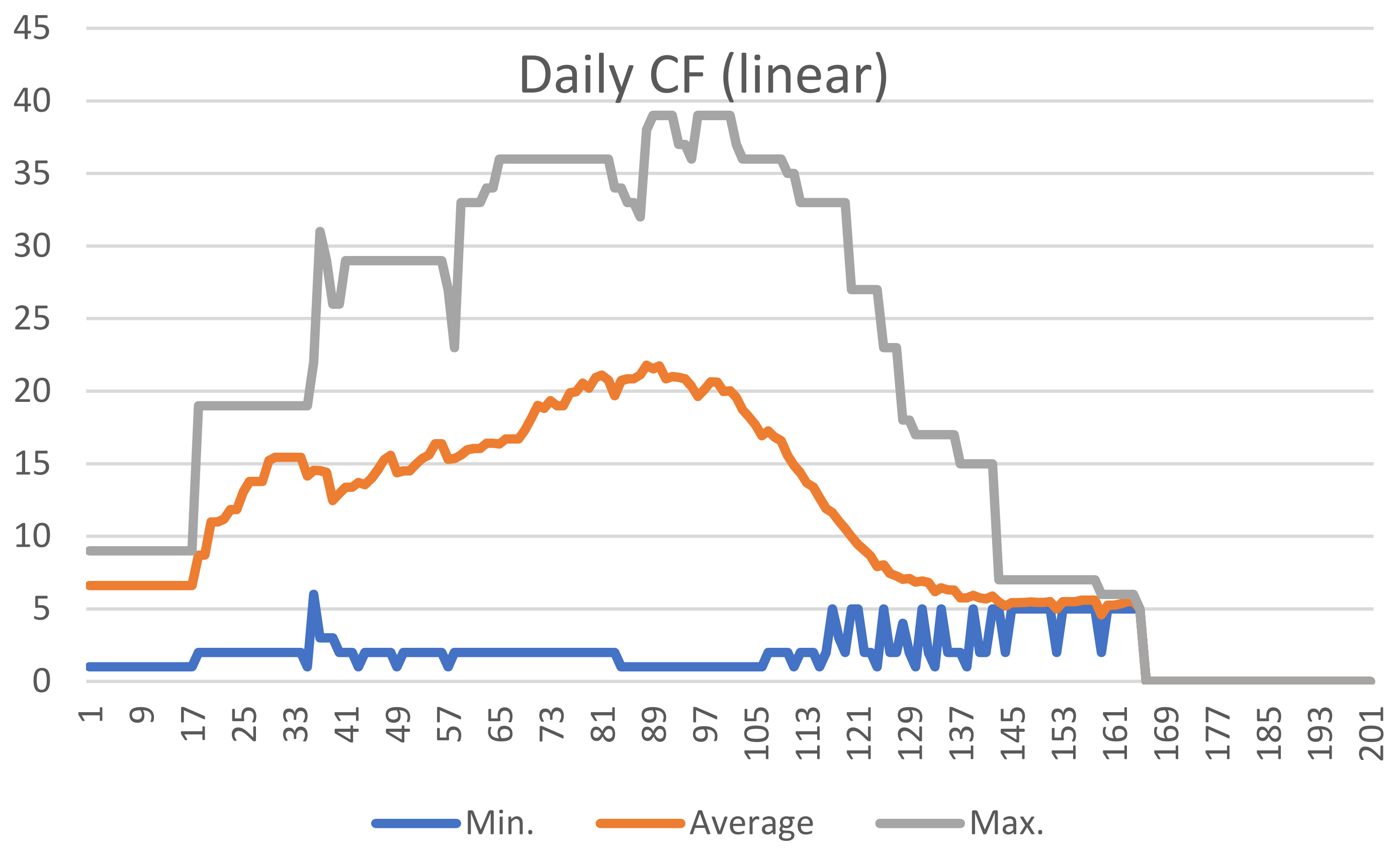
2.4. Time Series of Production Speeds-Simulation

The Cash Flow [24] is shown in Figure 3 for the linear (upper(a) part) and logistic (lower(b) part) resource distribution for activities A. The individual phases of the waveforms in the graphs are shown for 100 simulations.

The comment blocks in the context of G_Org(A) are marked as separately, and further supplemented by comments (a) Com 1–6, (b) Com 1–4. A visual comparison between the 2 parts of Figure 3 indicate significant differences between the linear distribution of resources (financial resources Q in terms of costs C) and the use of logistics functions of the distribution of resources C.

2.4.1. Linear Resource Drawing Schedule—Comment

• Com 1: The start of the project assumes a jump in production capacity. The jump increase does not correspond to the practice of implementation.
• Com 2: The onset of follow-up activities A_i misses the follow-up to the ongoing start-up activities; changes are needed in G_Org(A).
• Com 3: Some follow-up activities do not continue in parallel with ongoing activities. For some activities, the production speed decreases. The opportunity to increase production speed steadily is wasted.
• Com 4: Organizational and technological continuity of activities lead to disturbances in the flow of production speeds. A decrease to the level of the start of implementation can be expected with the concurrence of some external influences. Increasing production speed seems unworkable.
• Com 5: The consequences of the missed opportunities commented on in points 1 to 4 lead to congestion of activities. The expected consequences are chaotic states of coordination of activities, space constraints during implementation, defects in the quality of execution, and more.
• Com 6: A wide range of project completion dates, the completion slippages represent about 1/3 of the total project duration.

A change in the method of financing is chosen as a variant solution. The linear distribution of the funding source is to be replaced by another resource distribution curve; this example uses a logistic curve. Individual activities differ mainly in the pace of development and termination of production processes.

2.4.2. Comment for the Schedule of Drawing Resources by the Logistics Function

• Com 1: The achieved pace of implementation is not used to establish follow-up activities. The dynamics of implementation speeds are lost.
• Com 2: Individual activities start with a time delay. The achieved realization speeds are not linked in such a way that there is an effect of increasing the realization speed.
• Com 3: Activities that are supposed to create a precondition for the rapid completion of project implementation start with a time delay.
• Com 4: The finishing process is disorganized and extensive.

The weakness of the proposed implementation schedule of the investigated project is the low compactness (looseness) of the structure G_Org(A) in the implementation of the proposal.

In a similar way, it is possible to compare proposals for the implementation of alternative solutions (design, organizational, energy intensity, safety measures, and more).

2.5. Simulation of the Duration of the Project as a Whole D_A

Schematic model TAB_Project|Sim in Figure 2 and Figure 3 provides a variety of factual input data and calculated time series data [25]. In addition to the rate of utilization of resources is the knowledge about the potential of durations D_A volatility. Graphical presentation and statistical analysis of the time series [19] allows assessing the potential dynamics of external influences (for example, the expected development of material prices, wages, labor availability, traffic intensity, machinery, and other externalities). The durations are dominant application outputs of Figure 3, listed as {D_A}_Sim in Figure 4.

3. Analysis of Time Series Outputs

Time-schedule series obtained on the basis of TAB_Project creates decomposition time series data {Q_A1} to {Q′_t}_A1; {Q′_t}_A2; {Q′_t}_An, in Table 3, cost series for A₁ is {15; 15; 15; 15; 15; 15; 10}_A1. For A₂ linear decomposition is given as {12; 12; 12; 12; 12; 12; 3}_A2. Values for {Q″_t}_A, {Q‴_t}_A are further derived as differences. It indicates internal and external influences and their fluctuations. The idea used in practice is that the project schedule is compiled for the needs of technical execution of the work; i.e., for the contracting subject, it is the need to keep the proposed deadlines and estimated costs economical priority (including external resources such as the environment, future expected LCC costs of maintenance, renewal, modernization cycles, etc.) [26]. The robust economic framework of the contract is based on design, duration, costs. The fact is, regardless of the degree of sophistication of the proposals, the parameters of the introduced inputs are degraded due to external influences. The result is a degradation of confidence in the methodology for the processing time and cost schedules. Especially for projects with high demands on input resources (investments, innovations, etc.), exceeding the limits is a threat to the economic substance of the project [26]. For example, in [13], the authors evaluated the data of realized nuclear power plants in the US and described the state of the data for several decades as follows, “Relatedly, containment building costs more than doubled from 1976 to 2017, due only in part to safety regulations. Labor productivity in recent plants is up to 13 times lower than industry expectations”.

The authors formulate the conclusion that the results point to a gap between expected and realized costs stemming from low resilience to time- and site-dependent construction conditions [27,28].

On the one hand, large-scale projects shape the efficiency and effectiveness of national economic units [23]. On the other hand, they often exceed the limits of completion dates and costs. There is no doubt that the balance between economic intentions and implemented practice is disturbed. Equilibrium disorders affect both models of connected process theory and investment efficiency models. The disparity between the intention and the reality generally has devastating economic consequences.

The present study looks for early warning signals. Defects can lie in both the theory and the applied practice of the dominant technical and financial paradigm. The source of defects is, among other things, gaps in the harmonization of national versions of the legislation of the Building Laws of the EU countries and in the area of methods for solving time and cost schedules. There are a number of models for which practical application has not led to the desired results [7] and many cases where the application of the model (strategy, solution, project, and operation) in real conditions has led to devastating results [10].

The problem of non-standard behavior (let us call it nonlinear non-periodic oscillations) can be incorporated into the project design of the solution itself. This situation causes manifestations of instability and consequently chaos [29] in the implementation processes [30,31,32]. Early identification and classification of the problem can enable managerial measures and effective targeting. There are a number of diversified approaches to managing different processes over time, for example, optimization, formalization of operator sequences, etc. [33,34,35,36,37,38].

3.1. Information Potential

Output analysis allows the creation of volatility characteristics of terms and resource needs profiles. One of the profiling issues of the projects is the trend towards increasing or underestimating the expected use of resources. The illustrative example of Figure 4 shows the differences embedded in the linear or logistical distribution of resources for the individual project activities A_i.

Information for users lies in the knowledge of the space that opens up between the expected resource requirements {averQ′_t}_Sim and minimal {minQ′_t}_Sim, or maximum {maxQ′_t}_Sim resource requirements for the duration of the project. Tracing the material causes of resource requirements allows potential changes in specifications for the creation of qualified technical, organizational, and technological evaluations. The graph in Figure 5 evaluates a relatively wide-ranging data set of cash-flows {Q′_t}_Sim. It makes it possible to prevent disproportions in the budgeting of available resources during the preparation and implementation of the project. Finally, it enables changes focused on the design and decision-making of the management [39].

Visual comparison of the obtained waveforms indicates:

• More realistic dynamics of monitored processes with the distribution of resources based on the logistics function;
• The limits of high implementation speeds {maxQ′_t}_Sim, and their economic complexity;
• The limits of low implementation speeds {minQ′_t}_Sim; accompanying phenomena are slowing down or interrupting the implementation, organizational complexity of the project, errors in the preparation of the implementation, and more;
• Alternating cycles of the increase and slowdown of implementation with economic consequences;
• The unresolved continuity of implementation activities, especially {maxQ′_t}_Sim; their limiting manifestation may be both interruptions of project implementation and cycles in implementation speeds.

The defined space of the project implementation dynamics in Figure 5 between {minQ′_t}_Sim and {maxQ′_t}_Sim is a space for managing changes in implementation speeds (+/−). Change alone is not undesirable, but meeting the goal of the change is crucial. If it leads to the deterioration of some dimension of the quality of the project (read as environment, deadline, cost, integral benefit, etc.), the goal is in the wrong direction. Change as such is an opportunity—the potential for achieving a goal.

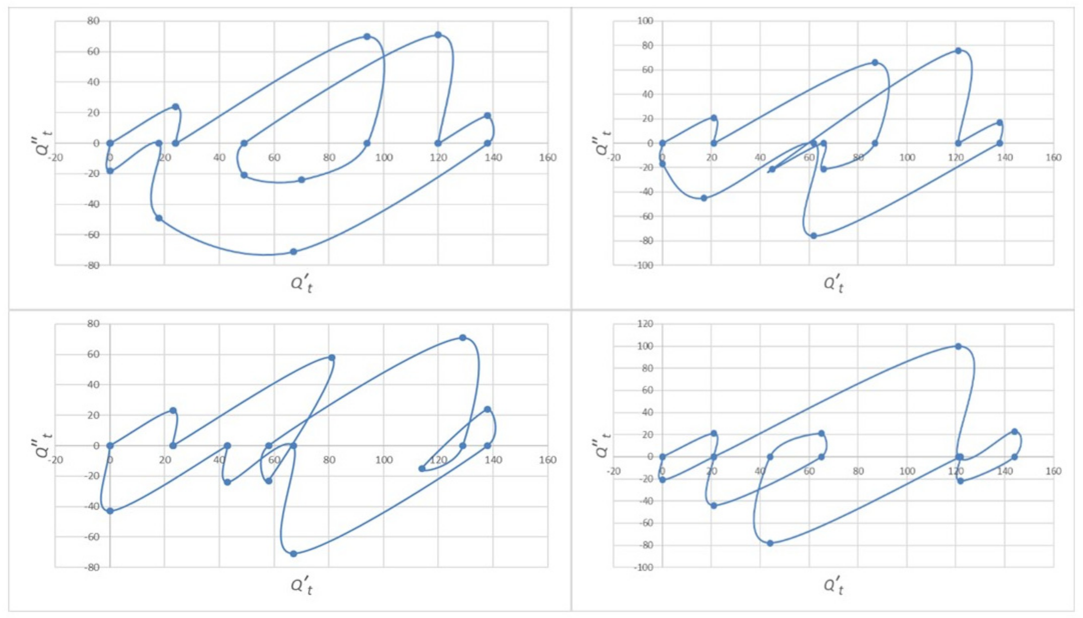
3.2. Phase Portrait Speed and Acceleration

The individual simulation time series outputs based on the dynamic model in TAB_Project make it possible to create a number of purpose-oriented project characteristics. Behavior of the time schedule model, with a certain degree of simplification tolerance, can be assigned change and volume outputs in each interval t:

TAB_Project(A_t) ⇒ [{C_t}, {C′′_t}, {C′_t}]

(3)

In Figure 6, a phase portrait of the speed of realization is given through speed {Q′_t} and acceleration {Q′′_t}. The calculation is based on a linear distribution of resources for all activities A. Outputs are based on deterministic inputs and externalities. Entering the volatilities of the input parameters allows the calculation of their combinations and consequences on the outputs. The result is a wide range of output data. Volatility limits of the simulation unit TAB_Project(A)│Sim are indicated in Section 3.1. The outputs of the simulation spectrum of the data in TAB_Project provide a quick overview of the nature of the design with a phase portrait. They enable the orientation of the obtained results by looking at (a) the order of project implementation; (b) the consequences of acceleration volatility and acceleration of project activities A, projected into shortening project implementation time; (c) the consequences of phase portrait symmetry losses; and (d) a tendency to bifurcation.

The basic focus of the study is the time-cost schedule and extension of effectiveness indicators. The phase-portrait of acceleration against speed is a powerful tool for more insight into the problem. Both qualitative indicators require energy availability. The phase-portrait plot is, in a certain sense, an “energy” transfer certificate.

Assume that, in the project shown in Figure 6a,b, on the right are references to the ideal state for a selection of several other projects (e.g., technology, construction, etc.). The compared project in Figure 6b on the left needs substantially higher changes in production speed than project Figure 6b on the right. The requirements for changes in production speed demand costs, qualified management, and time to implement. The project in Figure 6b on the left does not have matched production rates. It indicates higher costs and more difficult management.

More rectifications are shown in Figure 7. The maximum implementation rate exceeds 190 units valuing resources per time unit t. Maximum acceleration required (+/−) reaches almost 100 units per time unit. The proposed reference proposal is demanding, both on the speed of implementation and on the ability to balance the continuous organizational structures of project implementation.

The presented alternative designs for selection shown illustratively in the phase portraits of Figure 7 show significantly lower production speeds, around 140 units. Acceleration of production speeds is also at the level of about 80 units, with the exception of the design segment in the southeast corner in Figure 7. Phase portraits {Q″_t} towards {Q′_t} allow their evaluation to specify energy intensity. The prerequisite is the incorporation of the functions of the economics of energy intensity of the implemented processes into the calculation TAB_Project. Phase portraits comparison may show hidden economic relations (cointegration, causality) in the project structure [37]. Graphical interpretation is used in other methods as a close returns test, which predicates the existence of an unstable situation [33]. The phase portraits method could be used for comparative techniques for time-series analysis tasks [25].

3.3. Application Potential

The scope for the use of indicators of the dynamics of time and resource schedules of economic and technical project proposals is extensive. It mainly concerns investment projects, innovation projects, strategic development projects related to public and private projects [40,41,42].

An example is the European Green Deal and its Action Energy, abandoning fossil fuels while reducing CO₂ in the EU. However, the cessation of mining is provoking extensive dynamic responses and the need for new technologies and resources. Active investment projects of the past create new investment commitments for the future. They allow the analysis and formulation of new starting points and solutions.

The time and resource feasibility of the study is based on the schedule of project proposal sources such as:

• revitalization, here a new design of the excavated space;
• potential, use of giant mining mechanisms on alternative projects;
• analysis, time and cost schedules of investments;
• life cycle projects, new investment projects.

The indicated application possibilities of dynamic schedules enable the completion of branch-based economic support.

4. Conclusions

The time schedule of project resources is a visualization of organizational, economic, and technical dependencies before the preparation of an investment project. It anticipates future implementation states and situations. It contains instructions for implementation and determines the evolution of the project during use. However, it can also be a source of introduced, unrecognized, even objectively unrecognizable mistakes.

The tools of so-called early warning and decision-making are fragmentary or even absent. They make many decisions as careful as they are wrong. The sources of mistakes are presented in [20] and can be mostly related to:

(a)

factual specifications of the proposal (for example, technical, economic, legal, ecological or technological, and other errors);

(b)

misleading specifications of time and resource preparation of project activities (engineering of multiple works, project weaknesses, responsibility for risks, etc.);

(c)

misleading dispositions with available project resources (substitution of design, certification, durability, energy intensity, emissions, and more).

The project solution is an entry into the future and does not yet exist in this space and time (implementation, use, deconstruction, economic and legal standards). It is an effort to overcome the burden of data acquired in the past in favor of the vitality of new solutions in the future. Changes, speed, acceleration become the defining side aspects. The project design serves to verify the efficiency and petrifies the increase in ex-ante benefits.

Research focus, expansion, and stability are issues discussed in economics. In investment projects, the acquisition of tangible and intangible assets is associated with time scheduling as one of the key documents. However, the priority is not significantly reflected in research projects. In the citation database Web of Science, the result for Time Scheduling for May 2021 is about 153,000 publication results. For Investment Time Scheduling, the capacity of the research effort decreases to approx. 1100 results and results for Investment Cost Time Scheduling further decrease to 0.6 thousand.

Timely indication and marking of narrow profiles, including economic consequences, is one of the prerequisites for creating projects with a predicate—green, smart, affordable, sustainable/circular/life cycle.

References

1. Hilton, B.C. A History of Planning and Production Control 1750 to 2000; Book Guild Ltd.: Lewes, UK, 2005; p. 296. ISBN 1857769961. [Google Scholar]
2. Dasović, B.; Klanšek, U. Integration of mixed-integer nonlinear program and project management tool to support sustainable cost-optimal construction scheduling. Sustainability 2021, 13, 12173. [Google Scholar] [CrossRef]
3. Zlatanovic, M.; Matejevic, B. Usage of dynamic plans in civil engineering of Serbia. Facta Univ.-Ser. Arch. Civ. Eng. 2011, 9, 57–75. [Google Scholar] [CrossRef]
4. Holton, G.A. Defining risk. Financ. Anal. J. 2004, 60, 19–25. [Google Scholar] [CrossRef] [Green Version]
5. Burch, H.A. Basic Social Policy and Planning: Strategies and Practice Method; The Haworth Press, Inc.: Binghamton, NY, USA, 1996. [Google Scholar]
6. Samuels, L.K. Chaos Gets a Bad Rap: Importance of Chaology to Liberty. Strike-The-Root. 18 February 2015. Available online: http://www.strike-the-root.com/chaos-gets-bad-rap-importance-of-chaology-to-liberty (accessed on 25 November 2021).
7. Crouhy, M.; Gaqlai, D.; Mark, R. Risk Management; McGraw-Hill: New York, NY, USA, 2001. [Google Scholar]
8. Bareiša, E.; Karčiauskas, E.; Mačikénas, E.; Motiejunas, K. Research and development of teaching software engineering processes. In CompSysTech ’07: Proceedings of the International Conference on Computer Systems and Technologies, Ruse, Bulgaria, 14–15 June 2007; ACM Press: New York, NY, USA, 2007; ISBN 9789549641509. [Google Scholar] [CrossRef]
9. Koulinas, G.K.; Demesouka, O.E.; Sidas, K.A.; Koulouriotis, D.E. A TOPSIS—Risk Matrix and Monte Carlo Expert System for Risk Assessment in Engineering Projects. Sustainability 2021, 13, 11277. [Google Scholar] [CrossRef]
10. Flemming, C.; Netzker, M.; Schöttle, A. Probabilistic consideration of cost and quantity risks in a detailed estimate. Bautechnik 2011, 88, 94–101. [Google Scholar] [CrossRef]
11. Jorion, P. Value at Risk: The New Benchmark for Managing Financial Risk, 2nd ed.; McGraw-Hill: New York, NY, USA, 2001. [Google Scholar]
12. Tichý, T.; Brož, J.; Bělinová, Z.; Pirník, R. Analysis of predictive maintenance for tunnel systems. Sustainability 2021, 13, 3977. [Google Scholar] [CrossRef]
13. Eash-Gates, P.; Klemun, M.M.; Kavlak, G.; McNerney, J.; Buongiorno, J.; Trancik, J.E. Sources of cost overrun in nuclear power plant construction call for a new approach to engineering design. Joule 2020, 4, 2348–2373. [Google Scholar] [CrossRef]
14. Mohamed, H.H.; Ibrahim, A.H.; Soliman, A.A. Toward reducing construction project delivery time under limited resources. Sustainability 2021, 13, 11035. [Google Scholar] [CrossRef]
15. Bush, T.A.; Girmscheid, G. Projektrisikomanagement in der Bauwirtschaft; Beuth: Berlin, Germany, 2014; p. 242. ISBN 9783410223153. (In German) [Google Scholar]
16. Beran, J.; Feng, Y.; Grosh, S.; Kulik, R. Long-Memory Processes, Probabilistic Properties and Statistical Methods; Springer: Berlin/Heidelberg, Germany, 2013. [Google Scholar]
17. Rychlik, K. The Theory of Real Numbers in Bolzano’s Handwritten Papers; Publishing House of the Czechoslovak Academy of Sciences: Prague, Czech Republic, 1962. (In Czech) [Google Scholar]
18. Harrod, F.R. An essay in dynamic theory. In The Economic Journal; Palgrave Macmillan: London, UK, 1939; pp. 14–33. [Google Scholar]
19. Beran, V.; Dlask, P.; Eaton, D.; Hromada, E.; Zindulka, O. Mapping of synchronous activities through virtual management momentum simulation. Constr. Innov. Inf. Process Manag. 2011, 11, 190–211. [Google Scholar] [CrossRef]
20. Beran, V.; Teichmann, M.; Kuda, F. Decision-making rules and the influence of memory data. Sustainability 2021, 13, 1396. [Google Scholar] [CrossRef]
21. Beran, V.; Teichmann, M.; Kuda, F.; Zdarilova, R. Dynamics of regional development in regional and municipal economy. Sustainability 2020, 12, 9234. [Google Scholar] [CrossRef]
22. Kuda, F.; Teichmann, M. Maintenance of infrastructural constructions with use of modern technologies. Vytap. Vetr. Instal. 2017, 26, 18–21. (In Czech) [Google Scholar]
23. Awad, T.; Guardiola, J.; Fraíz, D. Sustainable construction: Improving productivity through lean construction. Sustainability 2021, 13, 13877. [Google Scholar] [CrossRef]
24. Rosłon, J.; Książek-Nowak, M.; Nowak, P.; Zawistowski, J. Cash-flow schedules optimization within life cycle costing (LCC). Sustainability 2020, 12, 8201. [Google Scholar] [CrossRef]
25. Fulcher, B.D.; Little, M.A.; Jones, N.S. Highly comparative time-series analysis: The empirical structure of time series and their methods. J. R. Soc. Interface 2013, 10, 20130048. [Google Scholar] [CrossRef]
26. Tichý, T.; Brož, J.; Bělinová, Z.; Kouba, P. Predictive diagnostics usage for telematic systems maintenance. In 2020 Smart City Symposium Prague; IEEE Press: New York, NY, USA, 2020; ISBN 978-1-7281-6821-0. [Google Scholar] [CrossRef]
27. Flyvbjerg, B.; Bruzelius, N.; Rothengatter, W. Megaprojects and Risk—An Anatomy of Ambition; Cambridge University Press: Cambridge, UK, 2003. [Google Scholar]
28. Flyvbjerg, B.; Steward, A. Olympic Proportions: Cost and Cost Overrun at the Olympics 1960–2012; Said Business School Working Paper; University of Oxford: Oxford, UK, 2012. [Google Scholar]
29. Marwan, N.; Romano, M.C.; Thiel, M.; Kurths, J. Recurrence plots for the analysis of complex systems. Phys. Rep. 2007, 438, 237–329. [Google Scholar] [CrossRef]
30. Prigogine, I.; Stengers, I. Order out of Chaos, Man’s New Dialogue with Nature; Bantam Books: New York, NY, USA, 1984. [Google Scholar]
31. Holton, G.A. Time: The Second Dimension of Risk. Financ. Anal. J. 1992, 48, 38–45. [Google Scholar] [CrossRef]
32. Samuels, L.K. In Defense of Chaos: The Chaology of Politics, Economics and Human Action; Cobden Press: London, UK, 2014. [Google Scholar]
33. Mindlin, G.B.; Gilmore, R. Topological analysis and synthesis of chaotic time series. Physica D 1992, 58, 229–242. [Google Scholar] [CrossRef]
34. Kong, Q.; Lee, C.-Y.; Teo, C.-P.; Zheng, Z. Scheduling arrivals to a stochastic service delivery system using copositive cones. Oper. Res. 2013, 61, 711–726. [Google Scholar] [CrossRef] [Green Version]
35. Shvetsova, O.A.; Lee, J.H. Minimizing the environmental impact of industrial production: Evidence from South Korean waste treatment investment projects. Appl. Sci. 2020, 10, 3489. [Google Scholar] [CrossRef]
36. Liu, Z. Chaotic time series analysis. Math. Probl. Eng. 2010, 2010, 720190. [Google Scholar] [CrossRef] [Green Version]
37. Gu, Z.; Xu, Y. Chaotic dynamics analysis based on financial time series. Complexity 2021, 2021, 2373423. [Google Scholar] [CrossRef]
38. Teichmann, M.; Kuta, D.; Endel, S.; Szeligova, N. Modeling and optimization of the drinking water supply network—A system case study from the Czech Republic. Sustainability 2020, 12, 9984. [Google Scholar] [CrossRef]
39. Rodionova, E.A.; Shvetsova, O.A.; Epstein, M.Z. Multicriterial approach to investment project’s estimation under risk conditions. Rev. Espac. 2018, 39, 28–44. [Google Scholar]
40. Lehtonen, J.-M.; Appelqvist, P.; Ruohala, T.; Mattila, I. Factory scheduling: Simulation-based finite scheduling at Albany International. In Proceedings of the 2003 Winter Simulation Conference, New Orleans, LA, USA, 7–10 December 2003; pp. 1449–1455. [Google Scholar]
41. Szeligova, N.; Teichmann, M.; Kuda, F. Research of the disparities in the process of revitalization of brownfields in small towns and cities. Sustainability 2021, 13, 1232. [Google Scholar] [CrossRef]
42. Jíšová, J.; Tichý, T.; Filip, J.; Navrátilová, K.; Thomayer, L. The application of the latest territorial components for sustainable mobility in district cities. IOP Conf. Ser. Earth Environ. Sci. 2021, 900, 012012. [Google Scholar] [CrossRef]
Figure 1. Mapping of quantities Q, cost C, durations D, and integration to total costs. The TCProject and TDProject are calculated in Table 2 and Table 3, and Figure 2; transformed in the specification—(arrow symbols, inversion tool, standard, etc.) into a feasible economic interpretation. Source: adapted and extended from [19].
Sustainability 14 02828 g001
Figure 2. Dynamic schedule example: externalities based on GOrg(A), calculation of cost and duration.
Sustainability 14 02828 g002
Figure 3. Project multiple cash flows {Qt′}Sim (100 times), interpretation as production speed per time unit; comparative segments (a,b) show linear and logistic resource distribution function, comparative analysis.
Sustainability 14 02828 g003aSustainability 14 02828 g003b
Figure 4. Simulation of project time series durations {DA}Sim.
Sustainability 14 02828 g004
Figure 5. Cash flow—linear distribution, {minQt}Sim, {averQt}Sim, {maxQt}Sim.
Sustainability 14 02828 g005
Figure 6. Simulation for Time schedule TABProject output analysis: (a) {Qt} and (b) phase portrait: production process acceleration {Qt} to production speed {Qt}.
Sustainability 14 02828 g006
Figure 7. Acceleration of phase portraits {Qt} to the production speed{Qt} for linear distribution of resources A; loss of symmetry, simulation outputs are based on TABProject, impact of externalities is included.
Sustainability 14 02828 g007