Article

A Threshold Model of Tailings Sand Liquefaction Based on PSO-SVM

1
School of Civil Engineering, Liaoning Technical University, Fuxin 123099, China
2
Liaoning Key Laboratory of Mine Subsidence Disaster Prevention and Control, Liaoning Technical University, Fuxin 123099, China
3
College of Civil and Transportation Engineering, Hohai University, Nanjing 210003, China
*
Author to whom correspondence should be addressed.
Sustainability 2022, 14(5), 2720; https://doi.org/10.3390/su14052720
Submission received: 22 November 2021 / Revised: 22 February 2022 / Accepted: 22 February 2022 / Published: 25 February 2022

Abstract

:
The liquefaction of tailings sand caused by seismic loads is a major problem in ensuring the safety of tailings ponds. Liquefaction may cause uncontrolled fluidized failure of the dam body, causing considerable damage to the lives, property and environment of people downstream. In this paper, a prototype tailings sand is used as the material to consider the main factors affecting liquefaction (i.e., dynamic load, soil quality, burial and static conditions). By embedding acceleration, pore pressure and earth pressure sensors in the rigid design of the self-designed rigid model box, different types of seismic waves of different ground motion amplitudes (PGA) were induced in a shaking table test of tailings sand liquefaction. The seismic intensity, waveform (class II, III and IV seismic waves) and active earth pressure of the PGA characterizing dynamic factors were obtained, and the static factors were characterized. The dynamic shear stress ratio, the peak acceleration of the earthquake, the pore pressure of the drainage factor and the buried depth (overlying effective pressure) characterize the soil conditions. SPSS software was used to analyze the factor dimension reduction, and the most suitable factors for factor analysis were obtained. Particle Swarm Optimization (PSO) was used to optimize the parameters, and the improved PSO-SVM algorithm was compared with the existing genetic algorithm (GA) and grid node search (GS). The algorithm used in this paper is fast and has a relatively high accuracy rate of 92.7%. The established threshold model method is of great significance to predict the liquefaction of tailings sand soil under the action of ground motions and to carry out safety managemenin advance, which can provide a certain reference for the project.

1. Introduction

Tailings disposal has always been an important concern worldwide [1,2,3], with the goal of protecting the environment and people from the hazards associated with tailings storage. Currently, the upstream method is mostly used to construct tailings dams [4], but this makes the immersion line higher and leads to the sand in the dam becoming fully saturated. In addition, tailings sand is very sensitive to the ground motion load and prone to liquefaction deformation and even instability and damage. According to the statistical analysis by the World Commission on Dams (ICOLD), since the beginning of the twentieth century, more than 200 cases of tailings dam accidents have been recorded, and most of them were related to earthquakes since the saturated tailings are prone to liquefaction due to earthquake motions, which leads to local dam failure [5,6,7]. Therefore, the determination of liquefaction factors, the liquefaction potential of vulnerable areas and the prediction of possible damage are among the most important research topics in geotechnical earthquake engineering.
To date, many methods have been developed to determine the potential of sand liquefaction. However, most of these methods use some state to separate the nonliquefaction region from the liquefaction region to establish evaluation criteria based on the data obtained from in situ tests. For example, the standard penetration test (SPT), static penetration test (CPT), flat blade expansion test (DMTS), shear wave velocity test (SWV) and self-drilling side pressure test (SBPT) are the most commonly used test methods to predict the possibility of liquefaction [8,9,10,11,12,13]. However, the randomness, complexity and uncertainty of a soil mass make it difficult to adopt appropriate empirical equations for regression analysis [14,15,16,17,18]. Therefore, many experts and scholars try to develop simpler and more practical scientific analysis models to predict the possibility of liquefaction and establish methods to distinguish the liquefaction of sandy soil [19]:
In recent years, the soft computing method, especially the artificial neural network method [20,21,22,23,24], has been widely used in geotechnical engineering to determine the bearing capacity of shallow pile foundations, the settlement and stability of soil slopes and the behavior, such as compressibility parameters, in actual solutions. In addition, in the past 20 years, researchers have tried to use different artificial intelligence methods to predict the liquefaction potential of soil. Goh [25,26,27] proposed different Artificial Neural Network (ANN) models to predict soil liquefaction potential based on actual field records of SPT, CPT and shear wave velocity data. Juang and Chen [28] used historical databases including CPT measurements to evaluate the liquefaction resistance of sand with various ANN models. Rahman and Wang [29] developed a fuzzy neural network model for liquefaction potential evaluation by using a large database of liquefaction cases based on SPTs. Baziar and Nilipour [30] used ANN and back-propagation algorithms to determine liquefaction in different locations based on CPT results. Hanna et al. [31] proposed a generalized regression neural network model to predict the liquefaction potential of soil sediments using SPT-based data, including field tests of the 1999 Turkey and Taiwan earthquakes. Chern et al. [32] developed a fuzzy neural network model to evaluate the soil liquefaction potential of a CPT field database, which includes actual liquefaction records of more than 11 major earthquakes between 1964 and 1999. Erzin and Ecemis [33] proposed different ANN models to predict cone penetration and liquefaction resistance. Xue and Xiao [34] proposed a hybrid genetic algorithm (GA) and support vector machine (SVM) to predict soil liquefaction potential by using CPT-based field data from large earthquakes from 1964 to 1983. Xue and Liu [35] proposed two optimization techniques, a genetic algorithm (GA) and particle swarm optimization (PSO), to improve the performance of a CPT-based neural network model for the prediction of soil liquefaction sensitivity based on field data of large earthquakes from 1964 to 1983. Hoang and Bui [36] proposed a novel soft computing model named KFDA-LSSVM, (combines kernel Fisher discriminant analysis with a least squares SVM) to evaluate earthquake-induced soil liquefaction.
In summary, experts and scholars have conducted many studies on the liquefaction phenomenon of sand under a dynamic load, but tailings sand is neither cohesive soil nor noncohesive, and there are few studies on the liquefaction phenomenon after the complex solid-liquid-gas-chemical coupling action. Therefore, for the liquefaction of ore tailings, there is an urgent need to propose a comprehensive consideration of various factors, and the convergence rate is relatively fast to determine the liquefaction threshold. This article takes prototype tailings sand as the material, considers the main factors affecting liquefaction (i.e., the dynamic load, the soil and buried and static conditions), uses SPSS software for factor dimension reduction analysis in order to determine the most suitable for factor analysis of influencing factors. It then uses the particle swarm method of parameter optimization (PSO) to generate into the support vector machine (SVM) for liquefaction condition prediction. The established threshold model method is of great significance for predicting the liquefaction of sandy soil under the action of ground motion, which can be used for reference in engineering.

2. Materials and Methods

2.1. Test Equipment

Given the destructive and unpredictable nature of earthquakes, it is very difficult to perform field tests directly. To study the flow characteristics of tailings after liquefaction under earthquake action, based on the existing research results at home and abroad, a laboratory shaking table test was adopted [37]. The model test of tailings sand liquefaction was carried out by the ANCO R-232H seismic simulator of the Liaoning University of Engineering Technology. The data acquisition system used in the experiment was mainly divided into two parts: a DH-3817K dynamic and static data acquisition instrument was used for pore pressure and earth pressure data acquisition. Acceleration acquisition was performed using a DH-5981 dynamic data acquisition instrument [38].

2.2. Test Material

Tailings sand was selected from the Tongnai iron mine in Fuxin, Liaoning. The basic physical and mechanical indexes of the ore tailings are shown in Table 1, and the specific grading curve is shown in Figure 1.
According to the research [39], the vibration process of tailings sand was divided into two stages, and the dynamic strength of unsaturated tailings sand was greater than that of saturated tailings.
In addition, the preparation method of saturated sand was as follows:
(1) Before preparing the model, first arranged the pore pressure gauge, earth pressure gauge and accelerometer at the predetermined position of the model box by flexible arrangement;
(2) Injected a certain amount of pure water into the model box;
(3) Prepared the tailings sand layer in 10 layers, and the vibrating sand shaker evenly sprinkled the tailing sand from the sand outlet. In order to ensure the uniformity of the tailing sand layer, if unevenness occurred, the surface was smoothed in time;
(4) Controlled the height of the water surface to be 5 cm above the sand layer in each operation to ensure that the prepared tailing sand was in a saturated state (maximum thickness 75 cm). However, in order to simulate the saturation state of the tailings sand in the actual tailings dam more realistically, the tailings sand between 75–90 cm from the platform height was not saturated, to ensure that the tailings sand was in a half-saturated state;
(5) Performed the test after the elements were still for 24 h.

2.3. Test Model Box

Considering the advantages and disadvantages of rigid boxes, flexible boxes and shearing model boxes, an improved new rigid model box was proposed. The vibrating table model test of tailings sand was carried out to verify the applicability of the model box. The experimental results showed that the natural vibration frequency of the model tailings sand and box was 2.36 Hz after white noise scanning, and the natural vibration frequency of the model box before the test was 12.25 Hz. The natural vibration frequency of the model box after the test was 10.91 Hz. The fundamental frequency of the empty model box was 5 times involves the vibration frequency of the model box with tailings sand, which is much greater than 2 times. Therefore, the model box does not affect the vibration characteristics of the free area of the model tailings sand and does not generate a self-vibration phenomenon. The vibration frequency meets the test requirements of the vibrating table.
According to the advantages and disadvantages of the rigid box, the flexible box and the shear model box, the boundary of the test model box was processed as follows:
(1) Treatment of the friction bottom: First, in order to avoid the relative sliding of the tailings sand and the bottom of the steel box as much as possible and to ensure that the test tailings sand and the bottom of the model box have a good bond, the inner side of the bottom plate was sprinkled with gravel of different sizes to simulate a friction boundary.
(2) Sliding boundary treatment: To reduce the frictional resistance between the tailings sand and the wall of the model box as much as possible and improve the rigidity of the tailings sand, lubricating oil was applied to the inner wall of the model box along the vibration direction as the sliding boundary treatment.
(3) Flexible boundary treatment: In order to minimize the influence of the sidewall boundary of the model box perpendicular to the ground motion direction on the dynamic response of the tailings sand in the box, the sidewall of the model box was lined with molded polystyrene foam board as the flexible boundary treatment.
In addition, four rectangular pipes were welded vertically along the four corners of the frame. Each side was welded into an “x” shape with rectangular pipes. The model box can hardly be bent and deformed. It is difficult for the model floor and the bottom of the tailings to slip relative to each other, but due to the great restraint formed around it, the free shear deformation of the model tailings sand in the horizontal direction is inevitably restricted. On the basis of the rigid box, the tailings sand should not be bent or deformed horizontally during the design.
The 2-norm method was used to test the designed model box boundary effect. The 2-norm method formula is as follows:
α = x i x j x i = Σ ( x i x j ) 2 Σ ( x i ) 2
where: x i is the reference point acceleration (central acceleration); x j is the comparing point acceleration (boundary point acceleration). Both are the maximal acceleration values at these points, and “i” and “j” both represent different time moments.
As seen from the definition, the magnitude of α reflects the degree of deviation of the boundary point acceleration from the center point acceleration over the full time range. If α is 0, then the two signals are identical, and the boundary effect can be completely eliminated. As seen from Table 2, the boundary norm index of different types of seismic waves (El Centro wave, Traft wave and Shanghai wave) is below 10%, which meets the boundary design requirements of the model box. Among them, peak acceleration is the actual captured acceleration applied to the box. The reference point acceleration is the center acceleration. The comparison point acceleration is the boundary point acceleration.

2.4. Sensor and Measuring Point Arrangement

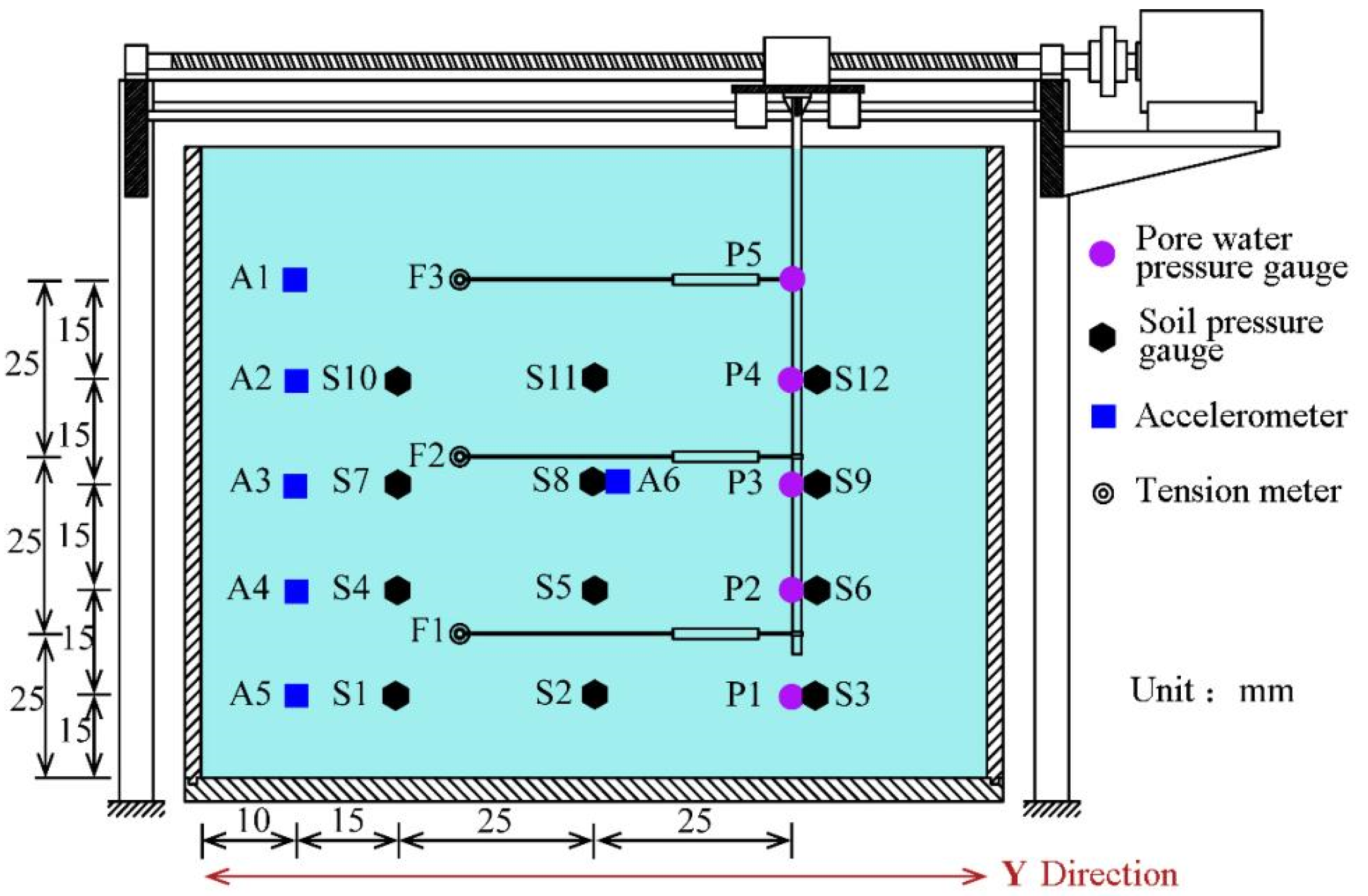
Considering that the traditional accelerometer arrangement method easily causes deflection and displacement of the sensor position when it is buried, the flexible arrangement sensor technology was used to arrange the sensors at equal intervals and equal depths at various key positions to ensure the scientific accuracy of the test. The test arrangement has five BS-1-type pore pressure sensors, six CE0-type piezoelectric voltage (IEPE) acceleration sensors, and 12 BX-1-type earth pressure sensors. Among them, the BS-1 piezometer has high sensitivity, good permeability and strong sealing; BX-1-type has a measuring range of 0.1MPa and an external dimension of Φ17 × 7 mm; On the one hand, CE0-type piezoelectric voltage (IEPE) acceleration sensors are processed to obtain accurate acceleration data from the front of the ground along the direction of the ground motion when it is buried. On the other hand, it must be sealed and waterproof. Therefore, the acceleration sensor is placed in a small box made of PVC board before the test and uses Special Kraft 304 silicone rubber for sealing and waterproofing; The range of GJBLS-1 tension sensor is 0-3kN. The sensor arrangement diagram is shown in Figure 2.

2.5. Test Loading Scheme

According to the geological survey report, a tailings pond is located in a 7-degree fortification zone with a preset seismic acceleration of 0.10 g and a characteristic period of 0.45 s. The equivalent shear wave velocity is greater than 284 m/s, which is a medium hard site [34]. A Traft wave is an actual strong earthquake record with a characteristic period 0.44 s, suitable for the medium hard site. Therefore, the Traft wave is preferred as the strong earthquake record in this test, and the corresponding amplitude adjustment was carried out according to the test plan. It is difficult to predict the evolution and destruction of the tailings in the tailings ponds at other types of sites. Therefore, to better study the dynamic response characteristics of different types of site tailings in the test, El Centro seismic waves for hard rock sites (Class II) and Shanghai waves for Class IV sites were selected according to the requirements of the specifications. Figure 3 is a time-history diagram of the input seismic wave acceleration to satisfy the actual seismic acceleration.
There is a related overview of vibration liquefaction in research and soil dynamics. The main factors affecting liquefaction are dynamic load conditions, soil conditions, burial conditions and static conditions.
In this test, the peak acceleration in the dynamic load factor was characterized by the peak acceleration actually collected by the acceleration. The magnitude was characterized by the ground motion intensity, PGA (0.1 g, 0.2 g and 0.3 g). The waveform was characterized by different local waves (II, III and IV), and the frequency was characterized by ground motion duration. The stress-strain history in soil factors was characterized by shear strain. The drainage conditions in burial factors were characterized by pore pressure changes, and the overlying effective stresses were characterized by buried depth. The shear stress in static conditions was characterized by the ratio of dynamic shear stress. The specific model test loading conditions are shown in Table 3.

3. Algorithm Design Based on PSO-SVM

3.1. Particle Swarm Optimization (PSO)

PSO is usually based on real coding and, due to the lack of cross-validation and variation, calculates the new speed based on its previous speed and the distance from its current position to its own best historical position and the best position of its neighbor. In general, the value of each component in νi can be sandwiched within [νmin, νmax] to control excessive roaming of particles outside the search space. The particle then flies to a new position and repeats the process until it reaches its maximum algebra. The main parameters of the PSO algorithm include population size and algebra. The convergence of the algorithm is influenced by the number of particles in the group (larger groups require more iterations to converge) and the topological structure: strongly connected groups (with larger domains, for example) converge faster than loosely connected neighborhoods. Is it possible to find a unique set of algorithm parameters that work well in all cases? Based on the above considerations, the following empirical program is found to work in practice [40].

3.2. Support Vector Machine (SVM)

The support vector machine is a new type of machine algorithm commonly used for pattern recognition. The salient features of SVM are the lack of local minima, the sparsity of the solution, and the feature space using kernel functions. Most classifiers were previously classified using hyperplanes. However, support vector machines extend the concept of classification to situations where linear classification is not possible by mapping predictors to a new dimensional space. In most cases, only the wrong kernel will appear in these different categories. Therefore, it can be considered that the optimal position of the decision plane is found only in the calculation, and the linear boundary is obtained by the nonlinear transformation to obtain the optimization problem of the kernel function creation [40].

3.3. Algorithm Design

PSO-SVM algorithm construction:
(1) Selection of data: According to the vibration table test data, the analysis of the factors affecting liquefaction under ground motion was carried out, and the factors suitable for the prediction model were obtained.
(2) Sample establishment: Based on the factor analysis, the parameters of the suitable influencing factors were analyzed, and the corresponding data were normalized. Then, the historical step number m and the predicted step number n were determined, thereby establishing learning and test samples, respectively.
(3) Initialization of data: Based on the particle swarm method, the initialization of the particle swarm parameters is performed, that is, the population size, the total number of iterations to be performed, the initial random values of the particles x 0 i and the velocity v 0 i were set. This included a particle vector representing an SVM model that corresponded to different penalty factors C and kernel function parameters g.
(4) Determine the search interval of (C, g).
(5) Found the fitness function of each particle: Calculate the particle fitness value in the group according to the objective function, compared the fitness value with the adaptation value of the more and more positions that were experienced, and obtain the best adaptation value:
f ( x ) = min [ max ( | x j x j | x j ) ] , j = 1 , 2 , , n
where x j the measured value of the j-th sample; x j the predicted value of the j-th sample; and l—the number of samples.
(6) According to the particle swarm algorithm, the fitness value fi calculated according to Formula (2) is compared with the optimal solution f ( p b e s t i ) of the self. If so, f ( p best i ) > f i the fi at this time replaces the optimized value of the previous process and simultaneously updates the particles, namely: p b e s t i = x i , f ( p b e s t i ) = f i
(7) Compare the fitness value f ( p best i ) with the fitness value of the optimal position f ( g b e s t ) traversed by the population. If the result is smaller than the fitness value of the optimal position traversed by the population (i.e., f ( p b e s t i ) < f ( g best ) ), the position is taken as the optimal position and stored.
(8) Determined whether the fi or the number of iterations meets the preset criteria. The optimal penalty parameter C and kernel function parameter g will be selected at this time.
(9) On this basis, the PSO-SVM prediction mode is established, and the output data are obtained. The proposed model is implemented on the MATLAB R2018a platform.

4. Factor Analysis of Influence Parameters of Tailings Sand Liquefaction

According to the shaking table test data, the features affecting liquefaction under the action of ground motion were analyzed to obtain the features suitable for the prediction model. SPSS software was used for factor dimensionality reduction analysis to obtain the most suitable features for factor analysis.
Through the shaking table test, the liquefaction of tailing sand under an earthquake was studied under the influence of various time-space features. To find the key factors and to make a corresponding comprehensive prediction, it is necessary to analyze the influence of different predictors on the possibility of liquefaction. According to the results of existing experiments and the above results of factor analysis and correlation among features, this paper selects eight types of impact features.
Four main factors affecting the liquefaction of saturated sand were analyzed (dynamic load conditions, soil conditions, burial conditions and static conditions). Considering the above factors, combined with the experimental conditions and research purposes of this article, the following eight influencing indicators were selected: (1) Peak ground motion acceleration (PGA) is used to characterize seismic intensity; (2) Seismic types (Category II, III and IV seismic waves) to characterize the waveform; (3) Depth from the surface (buried depth) to represent the overlying effective pressure; (4) Actual acceleration (refers to the peak acceleration collected by each acceleration sensor); (5) Holding time (refers to the total duration of the earthquake); (6) Earth pressure (refers to the vertical stress component); whether the drainage characteristics and (7) Dynamic shear stress ratio (the ratio of shear stress to shear strain) characterized by (8) pore pressure as the influence characteristics of tailings liquefaction flow threshold under earthquake are suitable as the influence characteristics of liquefaction occurrence.
For these eight factors, the original data results of tailings sand liquefaction are shown in Table 4, and the degree of correlation between the factors is shown in Table 5. Among them, when the pore pressure ratio (the ratio of pore pressure to the initial earth pressure at the location of the pore pressure sensor) is greater than or equal to 1, it is considered to be in a liquefied state, and when the pore pressure ratio is less than 1, it is considered to be not liquefied. At the same time, the liquefaction of tailings sand is determined by 8 types of impact features.
The KMO test and Bartlett’s sphericity test were performed on the above variables. The results are shown in Table 6.
The KMO value is 0.537 > 0.5, which is barely suitable for factor analysis. Bartlett’s sphericity test gives an approximate chi-square of 155.182, a companion probability of approximately 0.000, and a significance of less than 0.05. Therefore, the null hypothesis of Bartlett’s sphericity test is rejected, and it is considered suitable for factor analysis, so the next statistical analysis is performed.
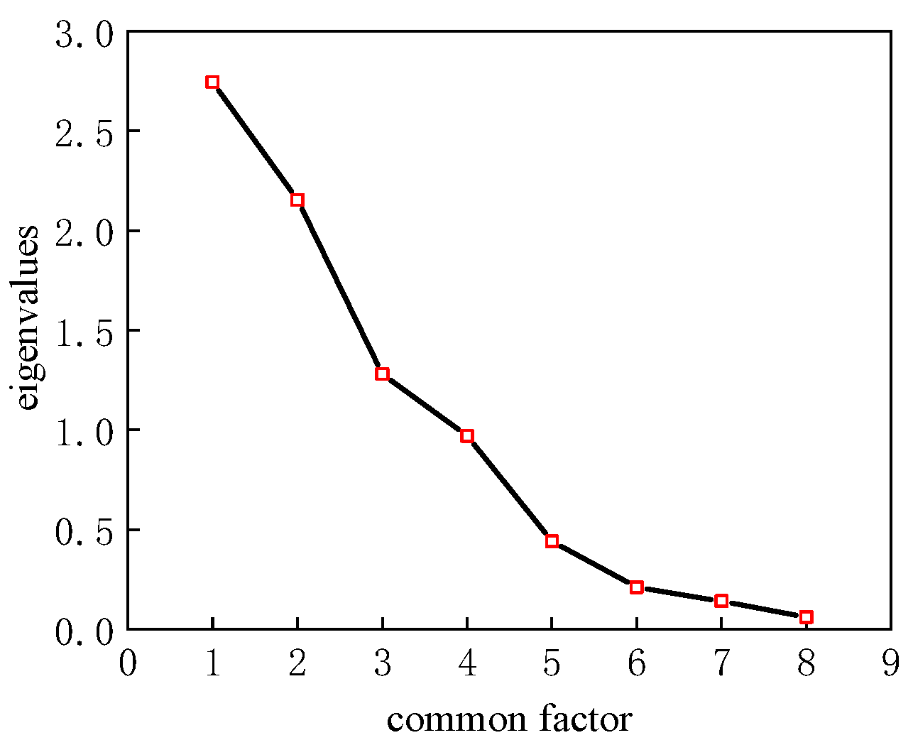
As shown in Figure 4, in general, the change in the feature value (refers to the influencing factors) is significant; that is, when the number of common factors increases to 8 feature values, it still shows a downward trend, which indicates that the eight influencing factors are important for factor analysis. Within the allowable range of error, the rate at which the feature values fall is slowed after six common factors, which indicates that the liquefaction possibility can still be described to some extent when analyzed with at least six influencing factors. This will be detailed and analyzed later.

5. Tailwater Sand Liquefaction Threshold Model Based on PSO-SVM

5.1. Normalization of the Influencing Factors

This paper focuses on the PSO-SVM algorithm to predict whether liquefaction will occur. Considering the difference in the dimensions of each influencing factor, the corresponding data magnitudes are also very different. Therefore, in the prediction of tailings liquefaction under earthquake action, each factor must be normalized to ensure the accuracy of the prediction. This paper normalizes using the following formula, where 0 means not liquefied and 1 means liquefaction:
x = x i x min x max x min
where: x is the value of the normalized factor; x i is the original value of the factor; x min is the minimum value of the factor; x max is the maximum value of the factor.

5.2. Construction of the Tailings Sand Liquefaction Threshold Model

The threshold model established in this paper mainly uses the data of nine working conditions preset in the experiment. That is, the input conditions of various working conditions and the data collected from each position sensor are set. This paper selects 22 data collection points, five different depths and nine working conditions, corresponding to a total of 45 kinds of results as samples. Take the normalized factor value as the network input and take the occurrence of liquefaction as the network output (0 means no liquefaction, 1 means liquefaction).
The initial parameters of the PSO model are shown in Table 7.
The PSO-SVM model constructed in this paper is first constructed by the RBF kernel. The two core parameters in the PSO are the penalty factor C and the kernel parameter g.
The entire liquefaction threshold model is established as follows:
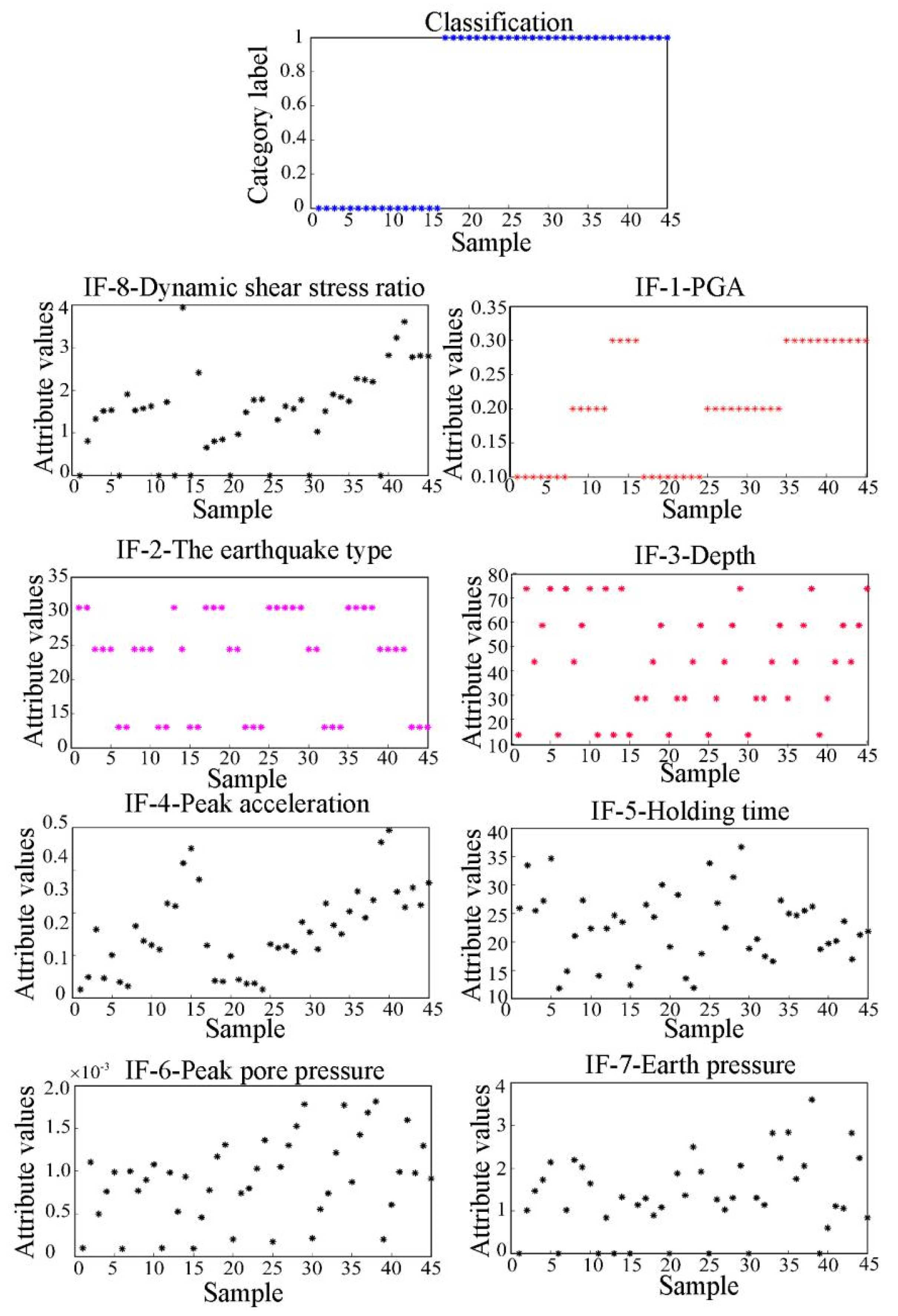
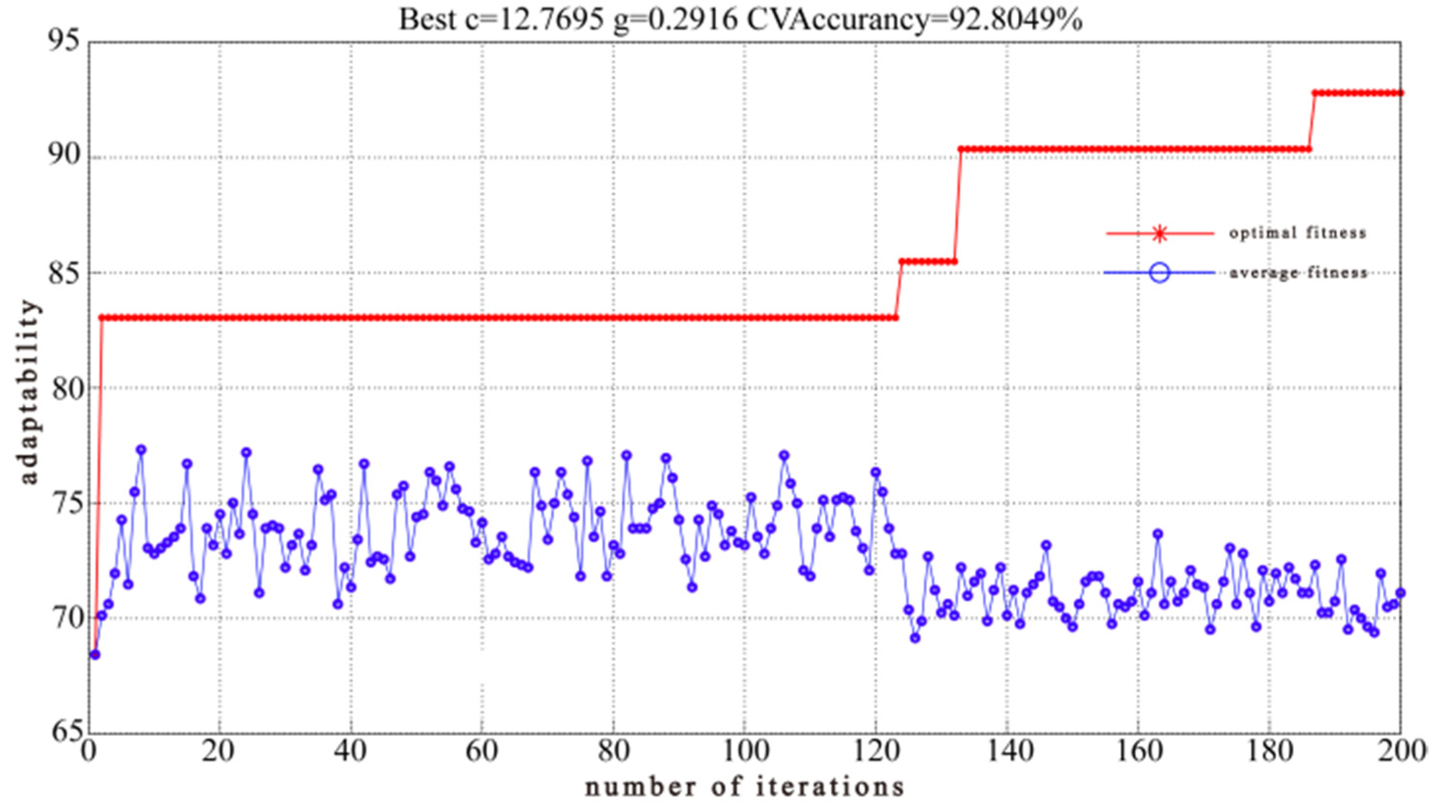
After the test data are imported into the program according to the implementation of the preset, the classification and all data normalization are automatically performed first. The data classification (liquefaction classification and influencing factor attribute classification) is shown in Figure 5. Then, the PSO will perform a global search, and the optimal parameters with the highest classification accuracy will be obtained. However, this process requires constant iterations and automatic searches until a satisfactory result position is reached. The parameters used in the PSO optimization process are given in Table 7, where the group size (Sizepop) is set to 20, the number of iterations (Maxgen) required is set to 200 and the inertia weight is set to 0.5. When the optimal parameters are found, a fitness curve for finding the best parameters is generated. If the best fitness is below the average fitness, the optimization fails; otherwise, the optimization succeeds. The size of the optimization accuracy depends on the maximum position of the best fitness. After the particle swarm optimization method is completed, the optimal parameters (penalty factor and kernel parameter) are obtained, and then automatically provided to the support vector machine program for corresponding training. After the completion of the training, the liquefaction condition is automatically predicted, thereby obtaining the actual situation. The test set and the corresponding prediction set are predicted according to the comparison between the prediction set and the test set.
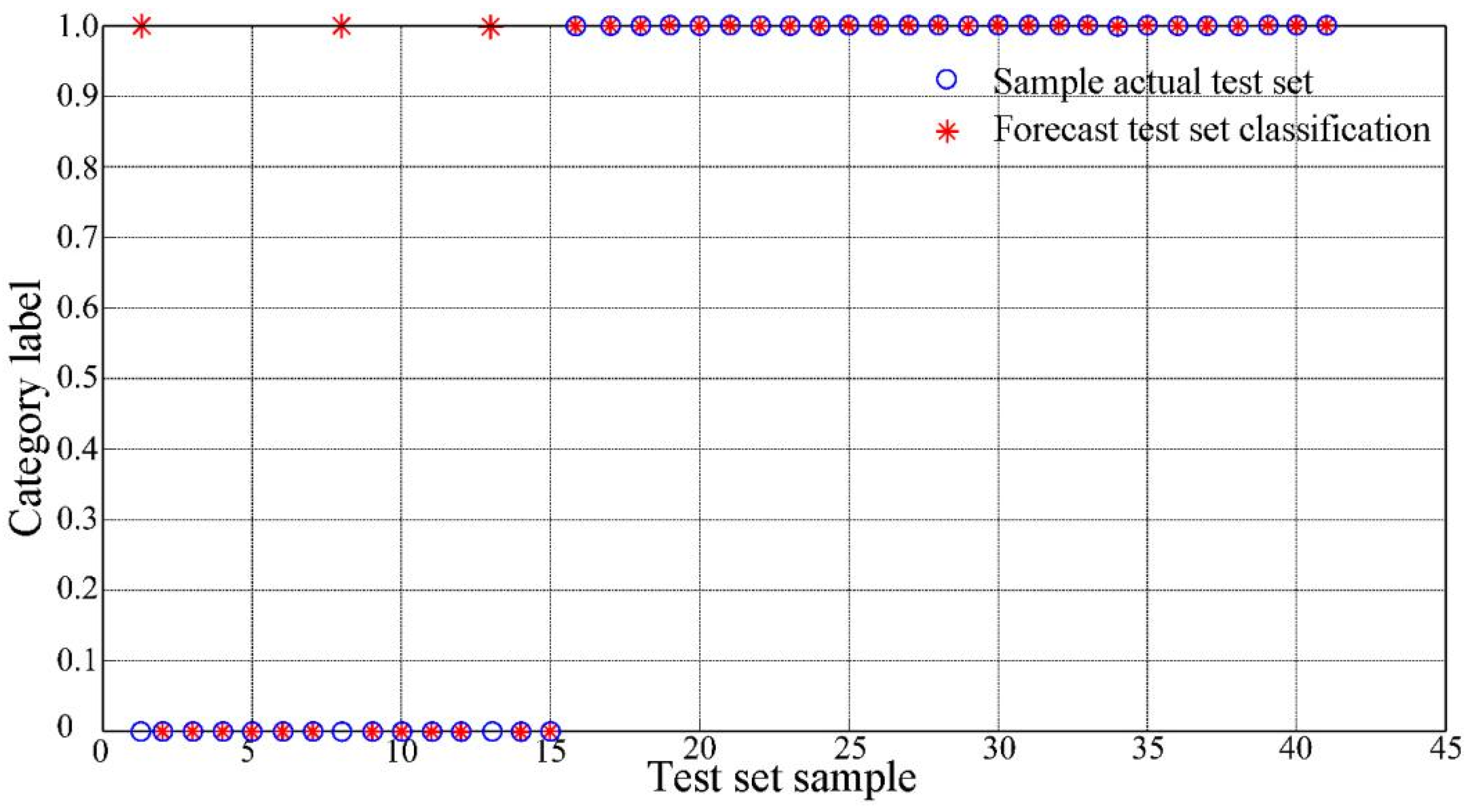
In order to fully verify the proposed optimized PSO-SVM model, in this paper, the data collected and sorted by all monitoring points under the nine working conditions in the test are first tested, with a total of 45 monitoring values. Figure 5 shows the liquefaction of 45 monitored values and the attribute values classified by eight influencing factors. Through the MATLAB program of PSO-SVM, the global penalty of the factor C and the kernel parameter g of the SVM model are obtained by the population particles. The optimal penalty factor of the SVM model suitable for seismic liquefaction under the experimental conditions is 12.7695. The kernel parameter is 0.2916, and the cross-validation rate is 92%, as shown in Figure 6. In this result, the SVM model is trained using the optimal parameters to generate the final classifier. Of the 45 test datasets used, only 3 were misclassified, and the overall classification accuracy rate was 92.7%, as shown in Figure 7. The designed PSO-SVM model has the ability to predict tailings liquefaction.

5.3. Analysis of the PSO-SVM Tailings Liquefaction Threshold Model

To verify the superiority of the PSO-SVM algorithm, the existing genetic algorithm support vector machine (GA-SVM) and grid search method (GS) optimized support vector machine (GS-SVM) algorithm are compared and calculated.
The genetic algorithm (GA), as an algorithm for survival of the fittest, natural selection and random genetic inheritance in the rules of source nature, has great advantages over traditional algorithms that cannot solve complex and other common nonlinear problems. At present, the GA has been widely used in various fields such as combinatorial optimization and has achieved some excellent results. Unlike traditional algorithms, this algorithm can search using randomly selected solutions without specifying an initial solution. It is similar to biological gene sequences and iteratively generates new solutions through certain selection, crossover and mutation operations. The use of chromosomes means that, like natural selection, there is a specific solution to each individual problem, and its quality is evaluated by fitness. The best ones are continuously selected to obtain excellent individuals. After that, the same process is used to breed the next generation, until after many generations of continuous updates, the results finally converge to obtain the optimal solution, and sometimes a suboptimal one.
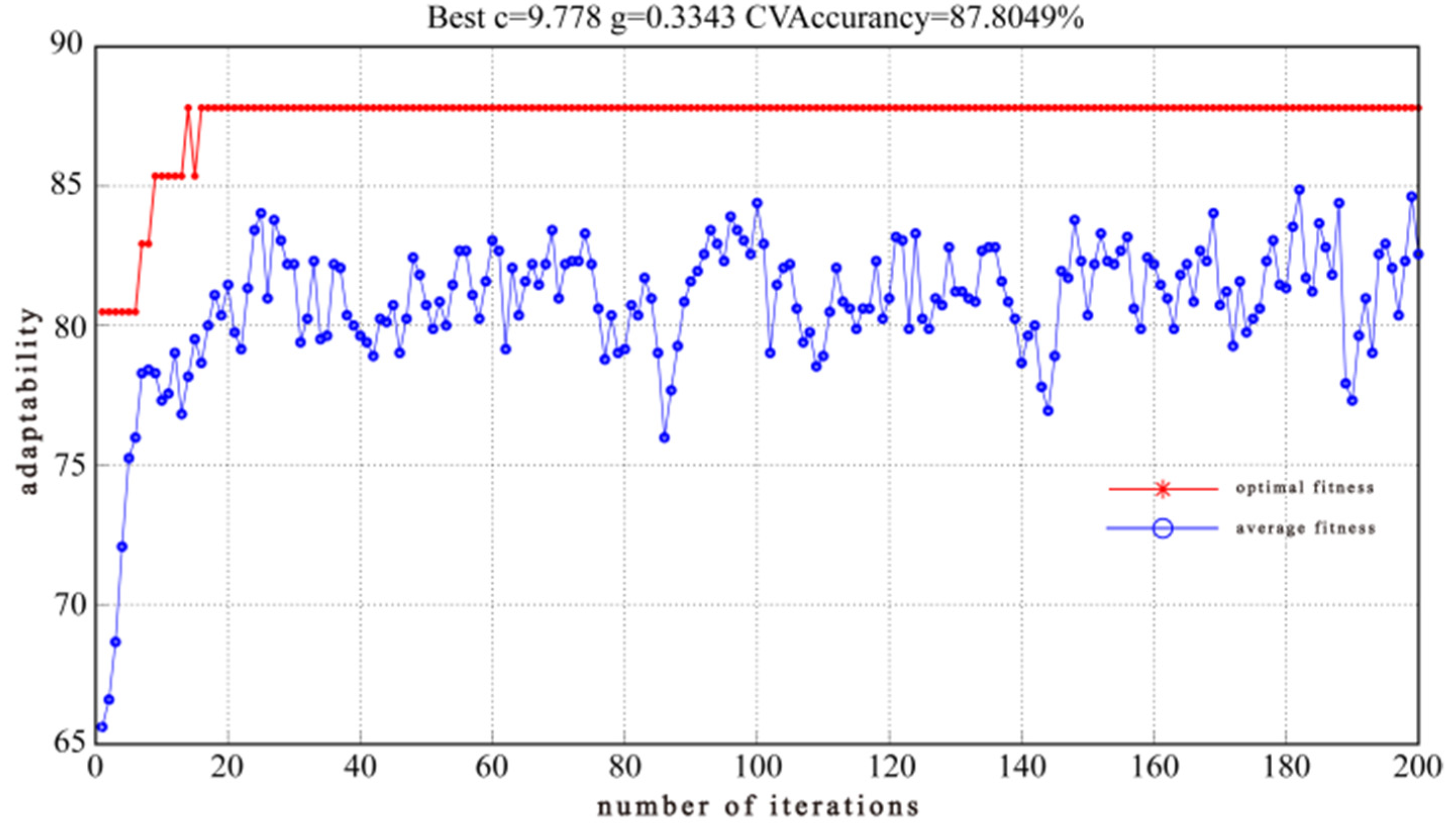
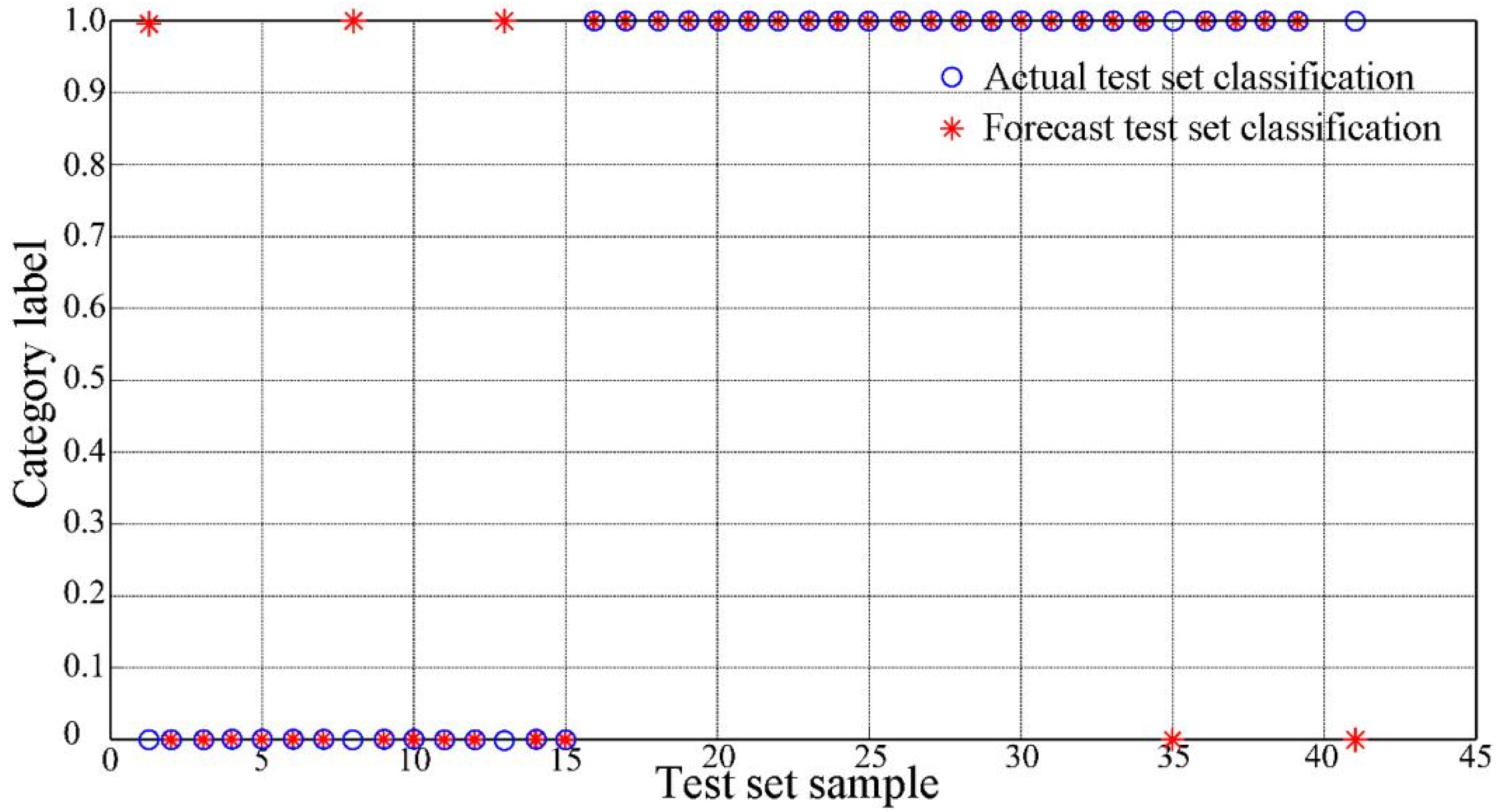
As shown in Figure 8 and Figure 9, the best (C, g) obtained by the GA-SVM algorithm is (9.778, 0.3343), and the cross-validation rate is 87.8%. In this result, the optimal parameters are used to train the SVM model to obtain the final classification results. In the 45 test datasets used, 5 samples were classified incorrectly, and the overall classification accuracy rate was 88.9%.
The GS algorithm performs an exhaustive search in the given data space to solve the model selection problem (i.e., find the optimal parameters for the dataset). However, since the boundary of the SVM parameter is a priori, the SVM parameter is first searched in the coarse range to find the optimal region of the SVM parameter. Once the coarse mesh search is completed, the fine mesh search is performed, but following the search process. The disadvantage is that the time is relatively long. The parameter ranges of the coarse mesh and fine mesh search are given in Table 8. After the grid search, the parameter with the highest classification accuracy will be selected for use by the SVM.
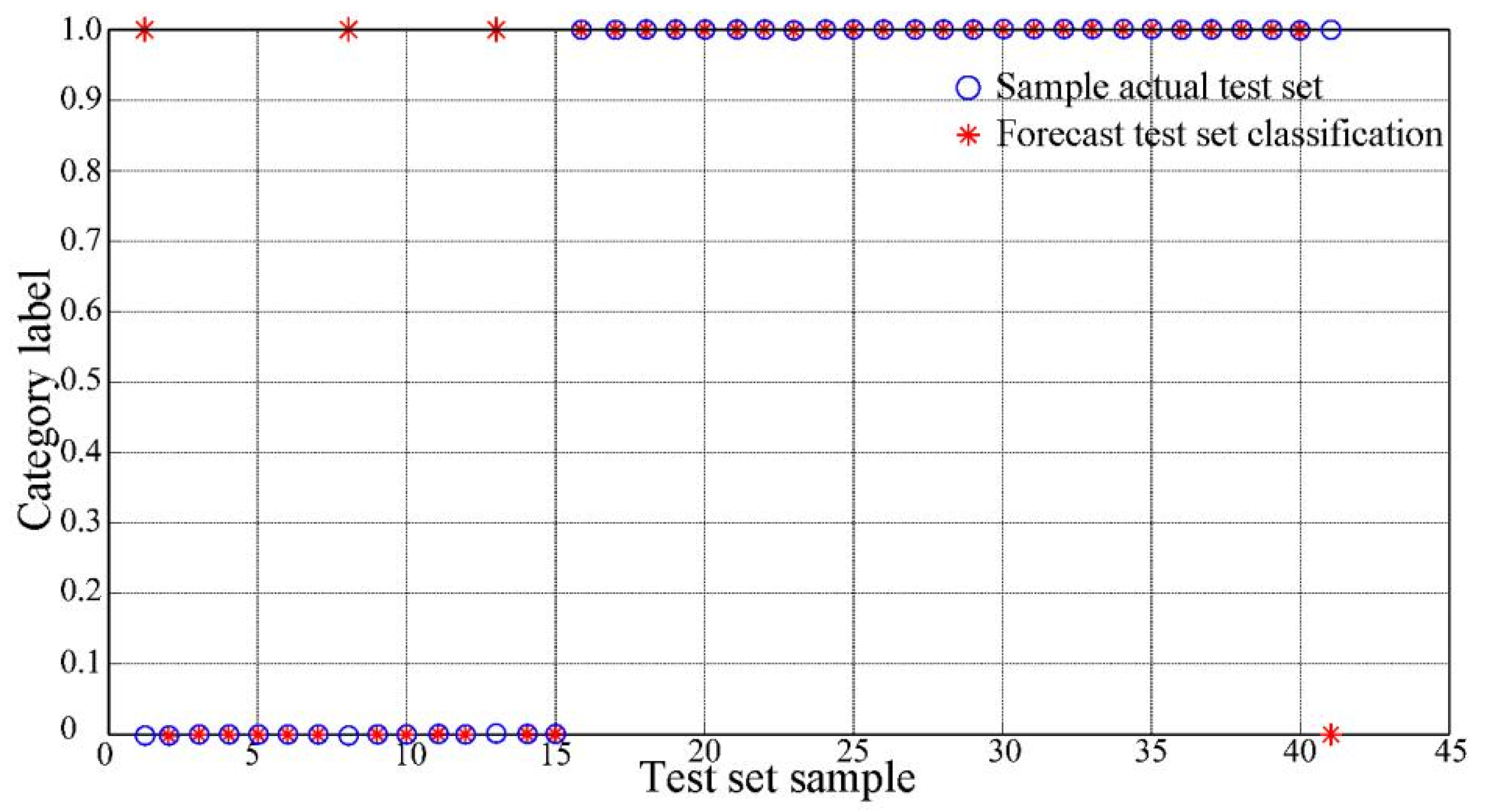
As shown in Figure 10, the best (C, g) obtained by the coarse grid search using the GS-PSO algorithm is (8, 0.5), and the cross-validation rate is 85.4%. Figure 11 shows that the best (C, g) obtained by the fine mesh search using the GS-PSO algorithm is (21.1121, 0.1436), and the cross-validation rate is 85.4%. In this result, the optimal parameters are used to train the SVM model to achieve the final liquefaction classification purpose. In the 45 test datasets used, 4 samples were classified incorrectly, achieving an overall classification accuracy of 91.1%, as shown in Figure 12.
To further study the accuracy of the PSO-SVM and GA-SVM and GS-SVM algorithms for predicting the seismic liquefaction threshold model, in addition to the test data used above, the working conditions of the seismic station model test are added, which enriches the model database.
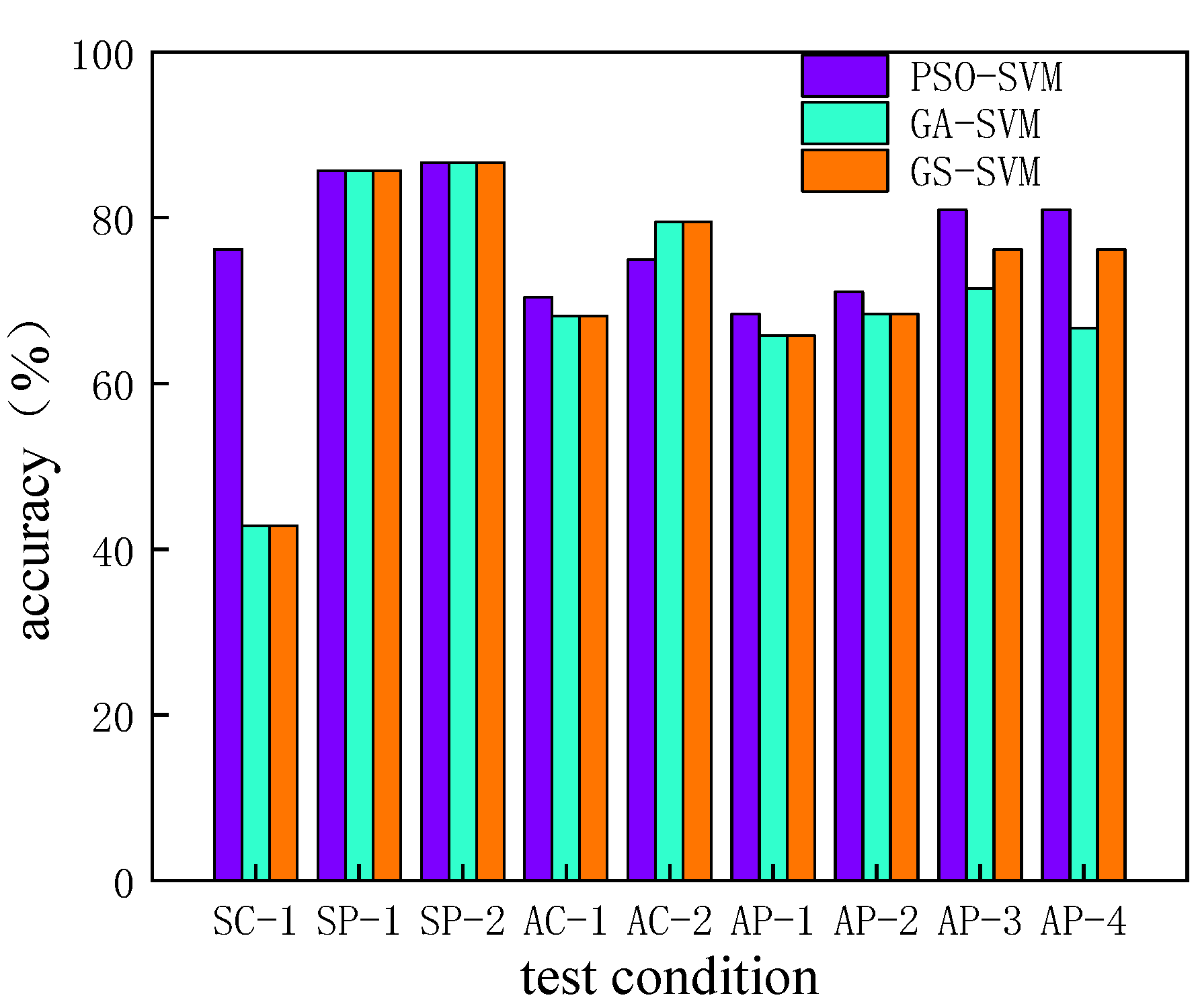
The newly used database combines the data used in the previous section with the addition of nine verification tests, a total of 18 trials with a total of 90 feedback data. SC-1 represents all the datasets in the second test (verification test), a total of 45; SP-1 represents part of the dataset in the second test, that is, a total of 36 after removing some missing data points; SP-2 indicates the test data points obtained by removing the factors that are relatively influential between each other (the peak acceleration of one test point is removed in this test) according to the factor reduction analysis and correlation statistics between the influencing factors.
Similarly, AC-1 represents a total of 90 points obtained after the combination of two experimental data (the first test data are used as the test set and the second test data are used as the prediction set); AC-2 indicates that 90 points have been dimension-reduced, that is, to remove the seven influencing factors and 90 points obtained by the relatively large correlation factors; AP-1 indicates the test points with 74 points after removing the missing data; AP-2 indicates that the AP-2 is based on AP-2. Data points after the dimension (seven influencing factors): AP-3 means not distinguishing the two experimental sequences with 90 points obtained by combination arrangement; AP-4 means seven influencing factors obtained after dimension reduction on the basis of the AP-3 data points.
The results are compared based on the results of PSO-SVM, GA-SVM and GS-SVM, as shown in Figure 13. It can be seen that the success rate predicted by the PSO-SVM algorithm is basically higher than that of the other two algorithms. In the least ideal case, the PSO-SVM method is almost similar to the prediction rate of the other two methods. Therefore, parameter determination and feature selection in PSO-SVM is very valuable. However, due to the limited space, this paper only uses the results database of the vibrating table indoor test to calculate the classification accuracy rate to evaluate the developed model. If possible, they should be applied in many ways to fully verify their innovative meaning. Therefore, in future research work, the model developed still has room for improvement.

6. Conclusions

In this paper, the prototype tailing sand was used as the material and the main factors affecting liquefaction were considered. Shaking table tests of tailings liquefaction were carried out with a self-designed rigid model box. The following conclusions were drawn:
(1) By performing a large number of factor analyses on the selected factors, the influencing factors suitable for the prediction model were obtained, namely: (PGA, Type of earthquake, buried depth, peak acceleration, holding time, peak pore pressure, peak earth pressure, and dynamic shear stress ratio)
(2) The particle swarm optimization method (PSO) was used to optimize the parameters, and the influencing factors were substituted into the support vector machine (SVM) to predict the liquefaction situation. The prediction accuracy of the liquefaction threshold model was improved and the prediction speed was accelerated.
(3) The improved PSO-SVM algorithm was compared with the existing genetic algorithm (GA) and grid node search method (GS), and it was found that the algorithm used is not only fast in calculation, but also relatively high in accuracy, reaching 92.7%, and has good applicability.

Author Contributions

J.J. is responsible for the theme control, theoretical analysis and experimental scheme design; S.Y. is responsible for the experiment and data collation; H.C. is responsible for the paper writing and later revision; B.J. and X.X. are responsible for the experiment. All authors have read and agreed to the published version of the manuscript.

Funding

National Natural Science Foundation of China (51974145), (51904144); Scientific Research Fund of Education Department of Liaoning Province (General Program): (LJKZ0354); Project Supported by Discipline Innovation Team of Liaoning Technical University (Key Laboratory of Civil Engineering Comprehensive Development and Utilization of Industrial Solid Waste in Sichuan Province): (SC_FQWLY-2020-Y-01).

Institutional Review Board Statement

Not applicable.

Informed Consent Statement

Not applicable.

Data Availability Statement

All data supporting the findings in this study are available from the corresponding author on reasonable request.

Conflicts of Interest

The authors declare that there is no conflict of interest regarding the publication of this paper.

References

  1. Senapati, P.K.; Mishra, B.K. Feasibility Studies on Pipeline Disposal of Concentrated Copper Tailings Slurry for Waste Minimization. J. Inst. Eng. (India) Ser. C 2017, 98, 277–283. [Google Scholar] [CrossRef]
  2. Karaca, O.; Cameselle, C.; Reddy, K. Mine tailing disposal sites: Contamination problems, remedial options and phytocaps for sustainable remediation. Rev. Environ. Sci. Bio/Technol. 2018, 17, 205–228. [Google Scholar] [CrossRef]
  3. Jin, J.; Qin, Z.; Lü, X.; Liu, T.; Zhang, G.; Shi, J.; Zuo, S.; Li, D. Rheology control of self-consolidating cement-tailings grout for the feasible use in coal gangue-filled backfill. Constr. Build. Mater. 2021, 316, 125836. [Google Scholar] [CrossRef]
  4. Moharrami, A.; Hassanzadeh, Y.; Salmasi, F.; Moradi, G.; Moharrami, G. Performance of the horizontal drains in upstream shell of earth dams on the upstream slope stability during rapid drawdown conditions. Arab. J. Geosci. 2013, 7, 1957–1964. [Google Scholar] [CrossRef]
  5. Fourie, A.B.; Blight, G.E.; Papageorgiou, G. Static liquefaction as a possible explanation for the Merriespruit tailings dam failure. Can. Geotech. J. 2001, 38, 707–719. [Google Scholar] [CrossRef]
  6. Wanatowski, D.; Chu, J. Static liquefaction of sand in plane strain. Can. Geotech. J. 2007, 44, 299–313. [Google Scholar] [CrossRef]
  7. Verdugo, R.; González, J. Liquefaction-induced ground damages during the 2010 Chile earthquake. Soil Dyn. Earthq. Eng. 2015, 79, 280–295. [Google Scholar] [CrossRef]
  8. Seed, H.B.; Idriss, I.M. Simplified procedure for evaluating soil liquefaction potential. J. Soil Mech. Found. Div. 1971, 197, 71–78. [Google Scholar] [CrossRef]
  9. Wu, K.; Shao, Z.; Qin, S.; Zhao, N.; Chu, Z. An improved non-linear creep model for rock applied to tunnel displacement prediction. Int. J. Appl. Mech. 2021, 13, 2150094. [Google Scholar] [CrossRef]
  10. Wu, K.; Shao, Z.; Sharifzadeh, M.; Chu, Z.; Qin, S. Analytical approach to estimating the influence of shotcrete hardening property on tunnel response. J. Eng. Mech. 2022, 148, 04021127. [Google Scholar] [CrossRef]
  11. Du, G.; Gao, C.; Liu, S.; Guo, Q.; Luo, T. Evaluation Method for the Liquefaction Potential Using the Standard Penetration Test Value Based on the CPTU Soil Behavior Type Index. Adv. Civ. Eng. 2019, 2019, 5612857. [Google Scholar] [CrossRef]
  12. Chu, Z.; Wu, Z.; Wang, Z.; Weng, L.; Liu, Q.; Fan, L. Micro-mechanism of brittle creep in saturated sandstone and its mechanical behavior after creep damage. Int. J. Rock Mech. Min. Sci. 2021, 149, 104994. [Google Scholar] [CrossRef]
  13. Ataee, O.; Moghaddas, N.H.; Lashkaripour, G.R. Estimating shear wave velocity of soil using standard penetration test (SPT) blow counts in Mashhad city. J. Earth Syst. Sci. 2019, 128, 66–91. [Google Scholar] [CrossRef] [Green Version]
  14. Abdi, Y.; Taheri-Garavand, A.; Sahamieh, R.Z. Prediction of strength parameters of sedimentary rocks using artificial neural networks and regression analysis. Arab. J. Geosci. 2018, 11, 587. [Google Scholar] [CrossRef]
  15. Sahu, S.P.; Patra, A.K. Development and assessment of multiple regression and neural network models for prediction of respirable PM in the vicinity of a surface coal mine in India. Arab. J. Geosci. 2020, 13, 890. [Google Scholar] [CrossRef]
  16. Chakraborty, A.; Goswami, D. Prediction of slope stability using multiple linear regression (MLR) and artificial neural network (ANN). Arab. J. Geosci. 2017, 10, 385. [Google Scholar] [CrossRef]
  17. Wu, K.; Shao, Z.; Qin, S.; Wei, W.; Chu, Z. A critical review on the performance of yielding supports in squeezing tunnels. Tunn. Undergr. Space Technol. 2021, 115, 103815. [Google Scholar] [CrossRef]
  18. Hu, B.; Sharifzadeh, M.; Feng, X.-T.; Guo, W.; Talebi, R. Role of stress, slenderness and foliation on large anisotropic deformations at deep underground excavations. Int. J. Min. Sci. Technol. 2021, 31, 577–590. [Google Scholar] [CrossRef]
  19. Zahmatkesh, A.; Noorzad, R. Investigation of monotonic and cyclic behavior of sand using a bounding surface plasticity model. Arab. J. Geosci. 2018, 11, 40. [Google Scholar] [CrossRef]
  20. Kimiaefar, R.; Siahkoohi, H.R.; Hajian, A.R.; Kalhor, A. Seismic random noise attenuation using artificial neural network and wavelet packet analysis. Arab. J. Geosci. 2016, 9, 234. [Google Scholar] [CrossRef]
  21. Wu, Y.-C.; Feng, J.-W. Development and Application of Artificial Neural Network. Wirel. Pers. Commun. 2017, 102, 1645–1656. [Google Scholar] [CrossRef]
  22. Farrokhi, F.; Firoozfar, A.; Maghsoudi, M.S. Evaluation of liquefaction-induced lateral displacement using a GMDH-type neural network optimized by genetic algorithm. Arab. J. Geosci. 2020, 13, 4. [Google Scholar] [CrossRef]
  23. Wu, K.; Shao, Z.; Sharifzadeh, M.; Hong, S.; Qin, S. Analytical computation of support characteristic curve for circumferential yielding lining in tunnel design. J. Rock Mech. Geotech. Eng. 2022, 14, 144–152. [Google Scholar] [CrossRef]
  24. Wu, K.; Shao, Z.; Qin, S.; Zhao, N.; Hu, H. Analytical-based assessment of effect of highly deformable elements on tunnel lining within viscoelastic rocks. Int. J. Appl. Mech. 2020, 12, 2050030. [Google Scholar] [CrossRef]
  25. Goh, A. Neural network modeling of CPT seismic liquefaction data. J. Geotech. Eng. 1996, 122, 70–73. [Google Scholar] [CrossRef]
  26. Goh, A. Probabilistic neural network for evaluating seismic liquefaction potential. Can. Geotech. J. 2002, 39, 219–232. [Google Scholar] [CrossRef]
  27. Goh, A. Seismic liquefaction potential assessed by neural networks. J. Geotech. Eng. 1994, 120, 1467–1480. [Google Scholar] [CrossRef]
  28. Juang, C.H.; Chen, C.J. CPT-based liquefaction evaluation using artificial neural networks. Comput. Civ. Infrastruct. Eng. 1999, 14, 221–229. [Google Scholar] [CrossRef]
  29. Rahman, M.; Wang, J. Fuzzy neural network models for liquefaction prediction. Soil Dyn. Earthq. Eng. 2002, 22, 685–694. [Google Scholar] [CrossRef]
  30. Baziar, M.; Nilipour, N. Evaluation of liquefaction potential using neural-networks and CPT results. Soil Dyn. Earthq. Eng. 2003, 23, 631–636. [Google Scholar] [CrossRef]
  31. Hanna, A.M.; Ural, D.; Saygili, G. Neural network model for liquefaction potential in soil deposits using Turkey and Taiwan earthquake data. Soil Dyn. Earthq. Eng. 2007, 27, 521–540. [Google Scholar] [CrossRef]
  32. Chern, S.-G.; Lee, C.-Y.; Wang, C.-C. CPT-based liquefaction assessment by using fuzzy-neural network. J. Mar. Sci. Technol. 2008, 16, 139–148. [Google Scholar] [CrossRef]
  33. Erzin, Y.; Ecemis, N. Thhe use of neural networks for CPT-based liquefaction screening. Bull. Eng. Geol. Environ. 2015, 74, 103–116. [Google Scholar] [CrossRef] [Green Version]
  34. Xue, X.; Xiao, M. Application of genetic algorithm-based support vector machines for prediction of soil liquefaction. Environ. Earth Sci. 2016, 75, 874. [Google Scholar] [CrossRef]
  35. Xue, X.; Liu, E. Seismic liquefaction potential assessed by neural networks. Environ. Earth Sci. 2017, 76, 192. [Google Scholar] [CrossRef]
  36. Hoang, N.-D.; Bui, D.T. Predicting earthquake-induced soil liquefaction based on a hybridization of kernel Fisher discriminant analysis and a least squares support vector machine: A multi-dataset study. Bull. Eng. Geol. Environ. 2018, 77, 191–204. [Google Scholar] [CrossRef]
  37. Jin, J.; Ding, Q.; Cui, H.; Zhang, P.; Xiao, X.; Lv, X. Dynamic response characteristics of a tailing dam determined by shaking-table tests. Arab. J. Geosci. 2020, 13, 897. [Google Scholar] [CrossRef]
  38. Jin, J.X. Study on Dynamic Characteristics of Upstream Tailings Pond under Seismic Load; Northeastern University: Shenyang, China, 2014. [Google Scholar]
  39. Liu, X.; Ji, Y.C.; Zhao, J.B.; Hou, S.W.; Hao, Z. Experimental study on liquefaction characteristics of tailing sand. Eng. Surv. Investig. 2015, 43, 15–18+24. [Google Scholar]
  40. Liu, X.K. Research on Damage Identification of Civil Structures Based on PSO-SVM; Jilin Jianzhu University: Jilin, China, 2021. [Google Scholar]
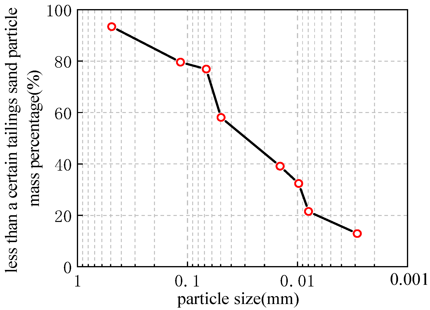
Figure 1. Screening curve of tailings sand particle size.
Sustainability 14 02720 g001
Figure 2. Schematic diagram of the sensor layout.
Sustainability 14 02720 g002
Figure 3. Seismic wave selection.
Sustainability 14 02720 g003
Figure 4. Common factor gravel map.
Sustainability 14 02720 g004
Figure 5. Liquefaction classification and influencing factors attribute classification.
Sustainability 14 02720 g005
Figure 6. PSO looks for the best parameter fit.
Sustainability 14 02720 g006
Figure 7. Comparison of PSO-SVM liquefaction prediction results with actual liquefaction results.
Sustainability 14 02720 g007
Figure 8. GA looks for the best parameter fit.
Sustainability 14 02720 g008
Figure 9. Comparison of GA-SVM liquefaction prediction results with actual liquefaction results.
Sustainability 14 02720 g009
Figure 10. Contour map of parameters C and g with accuracy (GS-SVM) (rough grid range).
Sustainability 14 02720 g010
Figure 11. Parameters C and g with accuracy (GS-SVM) (fine mesh range).
Sustainability 14 02720 g011
Figure 12. Comparison of GS-SVM liquefaction prediction results with actual liquefaction results.
Sustainability 14 02720 g012
Figure 13. PSO-SVM, GA-SVM and GS-SVM algorithm prediction accuracies.
Sustainability 14 02720 g013
Table 1. Physical and mechanical properties of the tailings sand.
PlasticityLiquid LimitPlasticity IndexOptimum Moisture
Content
Void RatioSpecific GravityMaximum Dry
Density
ωp/%ωl/%Ip/%ωop/%e/%G/g/cm3Ρdmax/g/cm3
13.1%20.57.414.20.8922.841.92
Table 2. Norm index of the input seismic wave model boundary of the shaking table.
Working ConditionSeismic WavePeak Acceleration
/m/s2
Reference Point Acceleration
/m/s2
Comparing Point Acceleration
/m/s2
Boundary Norm Index
/%
1II (El Centro)0.20.2460.2501.868
20.40.4570.4651.965
30.60.6650.6700.755
4III (Traft)0.10.1570.1581.061
50.30.3170.3407.652
60.50.5600.5661.245
7IV (Shanghai wave)0.40.4530.4530.011
80.20.2890.2841.653
90.40.4150.4549.282
100.50.5780.5800.335
Table 3. Model test loading conditions.
Site TypeSeismic WaveEarthquake Intensity (PGA)Working Condition
IIITraft0.1 g1
0.2 g2
0.3 g3
IIEl Centro0.1 g4
0.2 g5
0.3 g6
IVShanghai wave0.1 g7
0.2 g8
0.3 g9
Table 4. Raw data of tailings liquefaction.
PGA (g)Type of EarthquakeBuried Depth (cm)Peak Acceleration (g)Holding Time (s)Peak Pore Pressure (MPa)Peak Earth Pressure (MPa)Dynamic Shear Stress RatioLiquefaction State
10.1Traft−750.1230.90.0001————Unliquefied
20.1Traft−600.22431.520.00081.29320.6578liquefied
30.1Traft−450.14129.380.00120.89310.8068liquefied
40.1Traft−300.13935.020.00131.08490.84a91liquefied
50.1Traft−150.14938.460.00111.01040.8117Unliquefied
60.1El Centro−750.19924.120.0002————liquefied
70.1El Centro−600.14333.260.00071.87740.9701liquefied
80.1El Centro−450.26130.460.00051.46631.3297Unliquefied
90.1El Centro−300.14732.220.00081.72831.5168Unliquefied
100.1El Centro−150.20139.660.0012.1391.5355Unliquefied
110.1Shanghai wave−750.13816.820.0001————Unliquefied
120.1Shanghai wave−600.13418.560.00081.36461.4841liquefied
130.1Shanghai wave−450.13516.880.0012.49641.7746liquefied
140.1Shanghai wave−300.1222.920.00141.91911.7892liquefied
150.1Shanghai wave−150.12819.840.0011.0181.9084Unliquefied
160.2Traft−750.22638.820.0002————liquefied
170.2Traft−600.21831.820.0011.26641.3091liquefied
180.2Traft−450.22227.480.00131.0261.6283liquefied
190.2Traft−300.20936.380.00151.30191.5671liquefied
200.2Traft−150.27841.680.00182.05891.7761liquefied
210.2El Centro−750.25523.840.0002————liquefied
220.2El Centro−600.21525.480.00061.30661.0313liquefied
230.2El Centro−450.26926.040.00082.19321.53Unliquefied
240.2El Centro−300.23432.30.00092.02391.5746Unliquefied
250.2El Centro−150.22527.340.00111.63951.627Unliquefied
260.2Shanghai wave−750.21419.040.0001————Unliquefied
270.2Shanghai wave−600.32222.440.00071.13711.5094liquefied
280.2Shanghai wave−450.27121.580.00122.82461.9063liquefied
290.2Shanghai wave−300.2532.30.00182.23711.843liquefied
300.2Shanghai wave−150.32227.340.0010.83881.7258Unliquefied
310.3Traft−750.31629.640.0005————Unliquefied
320.3Traft−600.30329.960.00092.84061.7432liquefied
330.3Traft−450.3529.640.00141.74872.2737liquefied
340.3Traft−300.28930.480.00172.05382.2511liquefied
350.3Traft−150.3331.20.00183.60692.2024liquefied
360.3El Centro−750.46623.70.0002————liquefied
370.3El Centro−600.49324.70.00060.59752.8199liquefied
380.3El Centro−450.34925.160.0011.10913.2321liquefied
390.3El Centro−300.31328.620.00161.05873.6079liquefied
400.3El Centro−150.41628.460.00091.3233.9402Unliquefied
410.3Shanghai wave−750.45117.40.0001————Unliquefied
420.3Shanghai wave−600.37820.580.00051.13712.4138Unliquefied
430.3Shanghai wave−450.35921.940.0012.82462.779liquefied
440.3Shanghai wave−300.31826.220.00132.23712.8106liquefied
450.3Shanghai wave−150.3726.860.00090.83882.8Unliquefied
Table 5. Correlation matrix.
Influencing FactorPGAType of EarthquakeBuried DepthPeak AccelerationHolding TimePore PressureEarth PressureDynamic Shear Stress Ratio
CorrelationPGA1.000——————————————
Type of earthquake0.0001.000————————————
Buried depth0.0000.0001.000——————————
Peak acceleration0.873−0.083−0.0551.000————————
Holding time−0.1130.7190.388−0.1561.000——————
Pore pressure0.1390.1680.760−0.0450.3941.000————
Earth pressure0.153−0.0540.073−0.0050.0210.3371.000——
Dynamic shear stress ratio0.773−0.2700.2220.727−0.3010.1630.0411.000
SignificantPGA——0.5000.5000.0000.2010.1350.1870.000
Type of earthquake0.500——0.5000.3380.0000.0910.3770.056
Buried depth0.5000.500——0.3850.0110.0010.3370.097
Peak acceleration0.0000.3380.385——0.2170.3490.4880.000
Holding time0.2010.0000.0110.217——0.0150.4520.037
Pore pressure0.1350.0910.0010.3490.015——0.0210.182
Earth pressure0.1870.3770.3370.4880.4520.021——0.407
Dynamic shear stress ratio0.0000.0560.0970.0000.0370.1820.407——
Table 6. KMO and Bartlett test.
KMO Sampling SuitabilityBartlett Sphericity Test
0.523Approximate chi squareDegree of freedomSignificant
155.182280.000
Table 7. Parameters used in the PSO model.
Initial ParameterSizepopMaxgenLearning FactorLearning FactorInertia WeightPenalty Factor C Optimization RangeKernel Parameter g Optimization Range
Value202001.51.70.5[0, 200][0, 1]
Table 8. Parameter grid range in the SVM model.
SVM ParametersCoarse Grid RangeFine Mesh Range
C(2−5, 25)(2−2, 24)
g(2−10, 210)(2−4, 24)
Publisher’s Note: MDPI stays neutral with regard to jurisdictional claims in published maps and institutional affiliations.