
Techno-Economic and Environmental Impact Analysis of Large-Scale Wind Farms Integration in Weak Transmission Grid from Mid-Career Repowering Perspective

 , ,
, ,  ,
,  ,
,  and
and
Abstract
:1. Introduction
- LSWF integration in a deficient transmission grid, using Pakistan as a case study.
- Performance and cost–benefit analysis of various FACTS devices as a problem-solving solution.
- Scenario-based approach for dealing with PQ and Q compensation by appropriate and cost-effective FACTS devices as well as recovering power shortfalls by raising hub height with and without FACTS devices.
- A complete techno-economic impact evaluation of LSWF integration in terms of the environment.
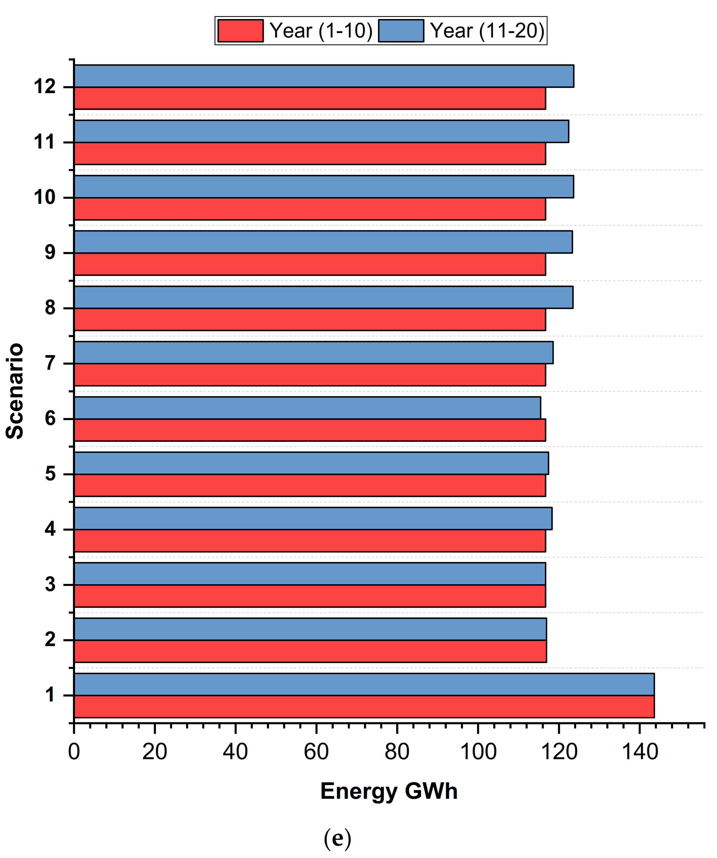
2. Energy Analysis
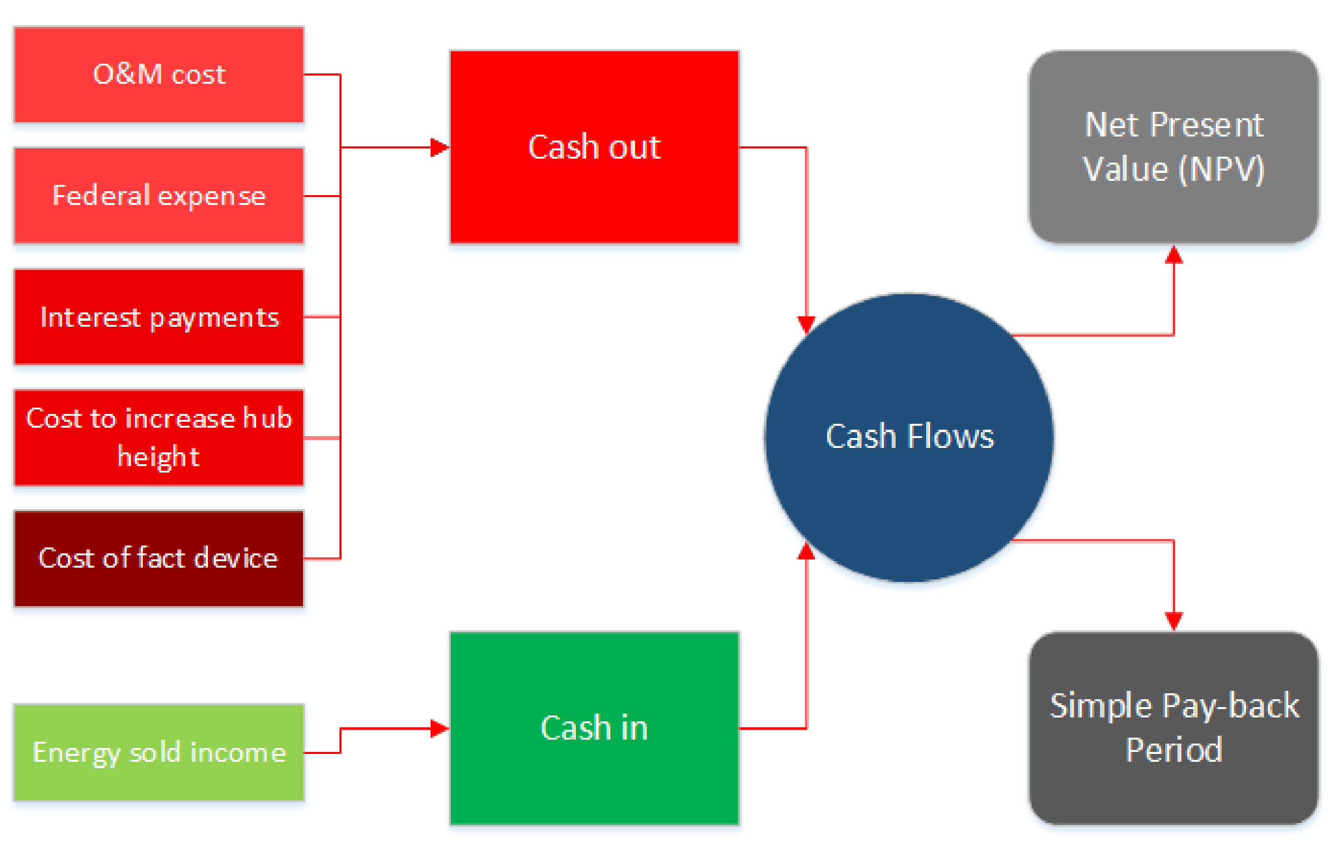
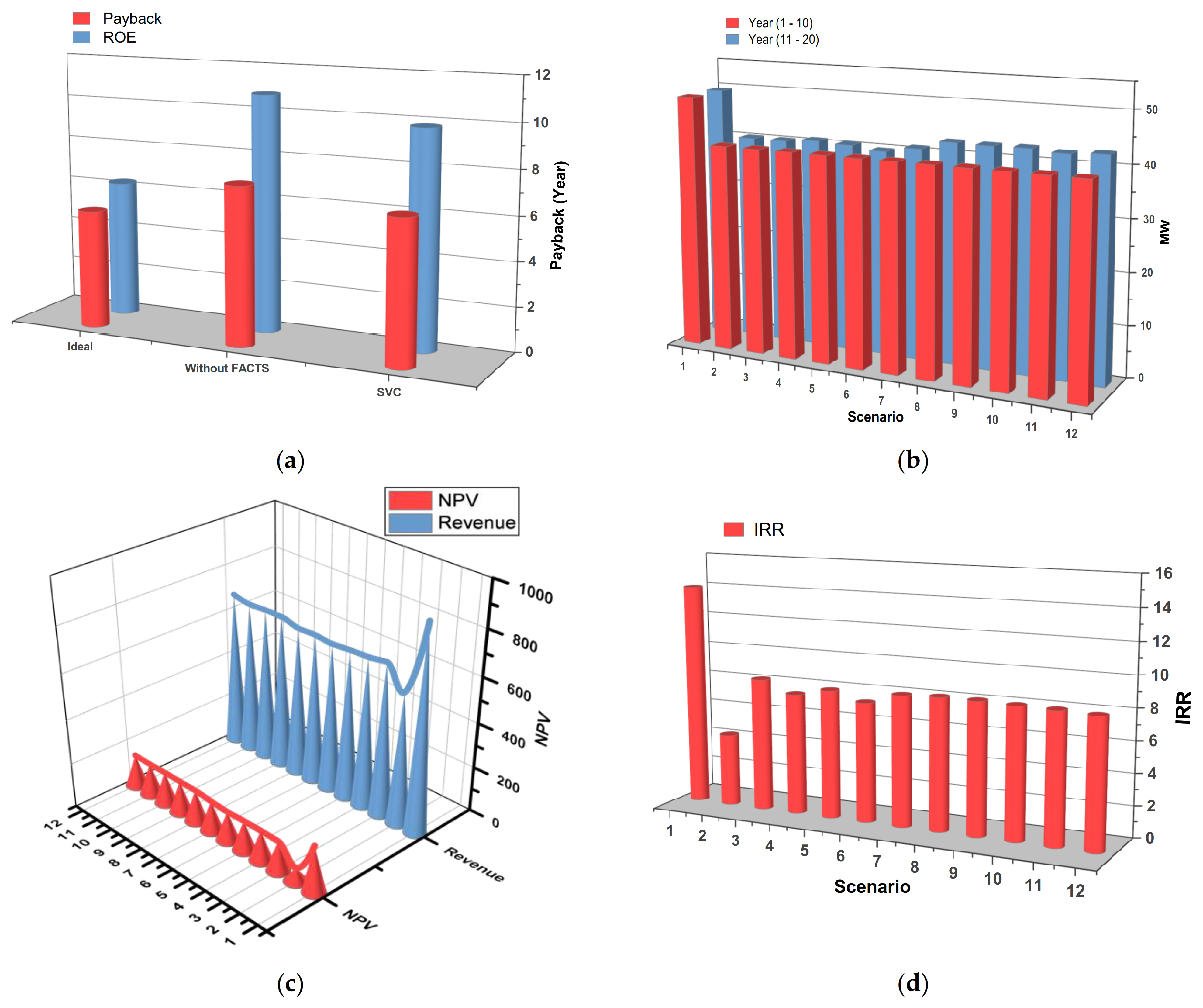
3. Economic Analysis
3.1. Simple Payback Period—SPP
3.2. Net Present Value—NPV
3.3. Internal Rate of Return—IRR
3.4. Capacitor Bank and FACTS Devices Cost Functions
3.5. HUB Height Cost Function
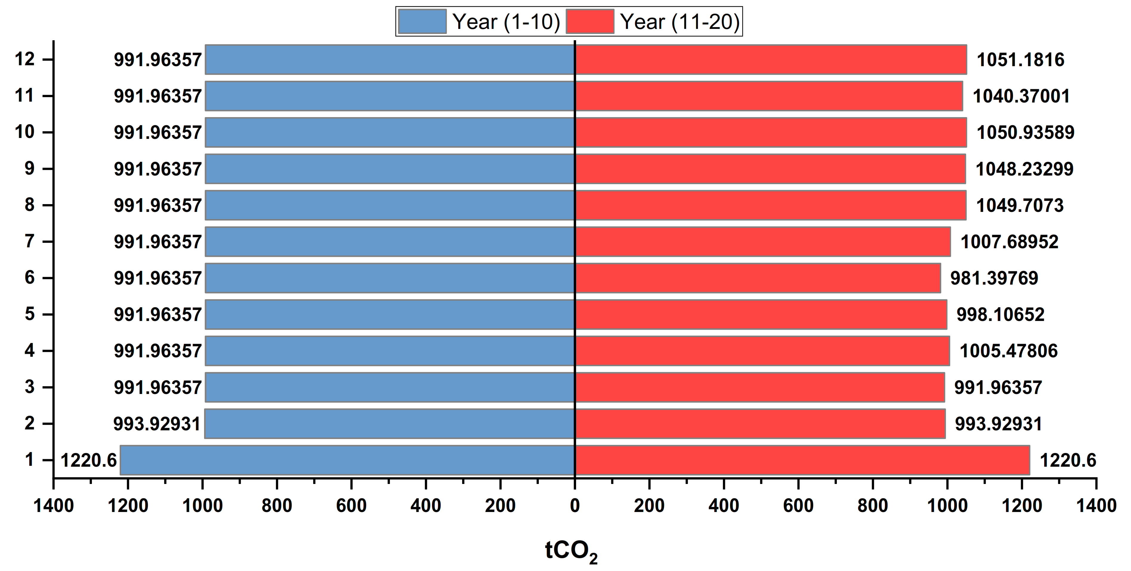
4. Environmental Analysis
5. LSWF Test Setup and Background Information
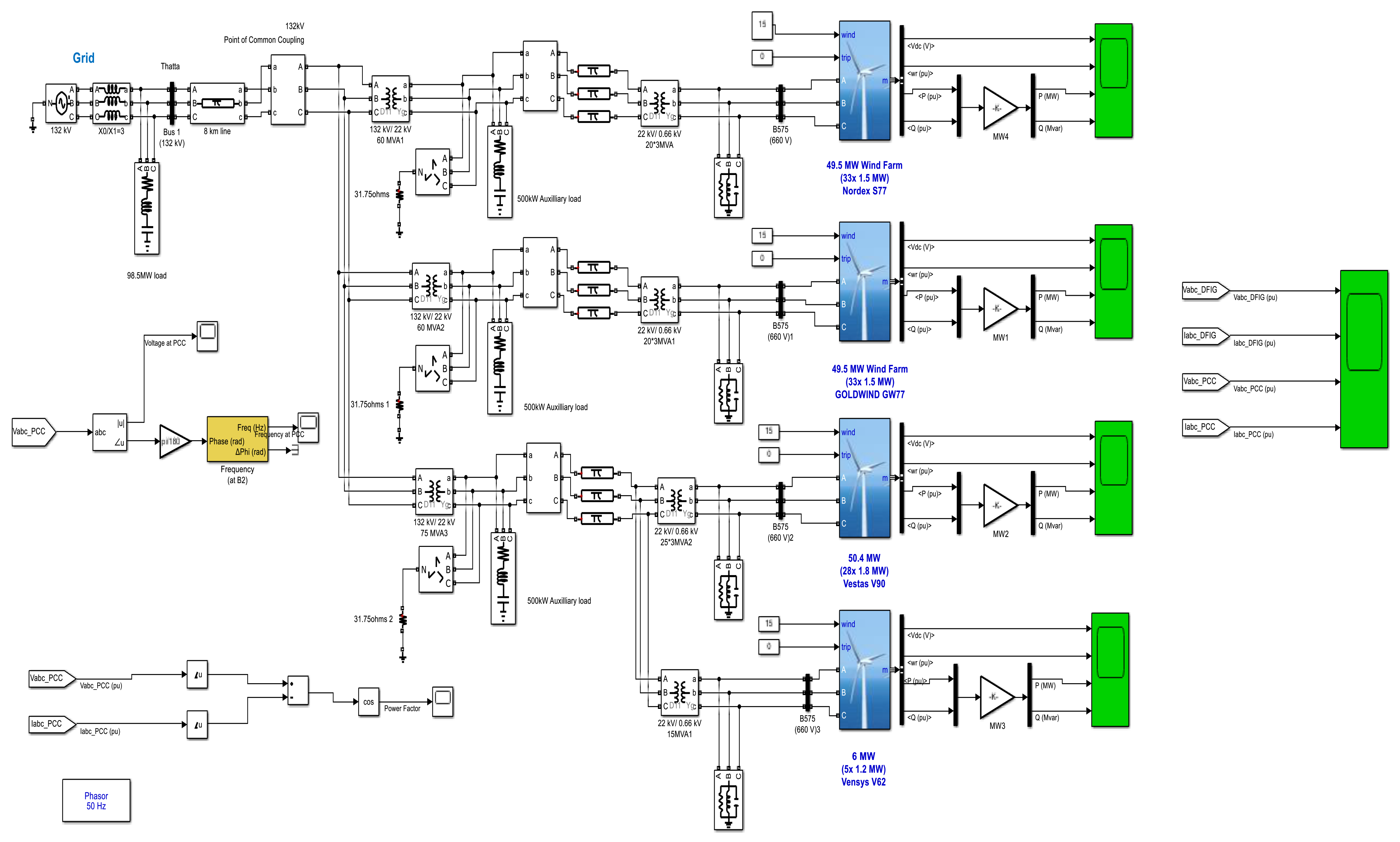
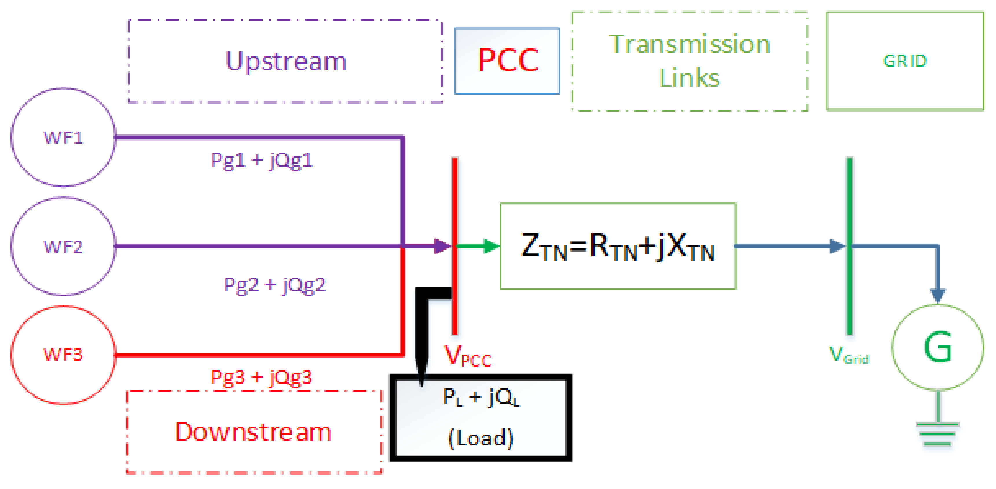
5.1. LSWF Test Setup
5.2. Grid Codes for Power Quality
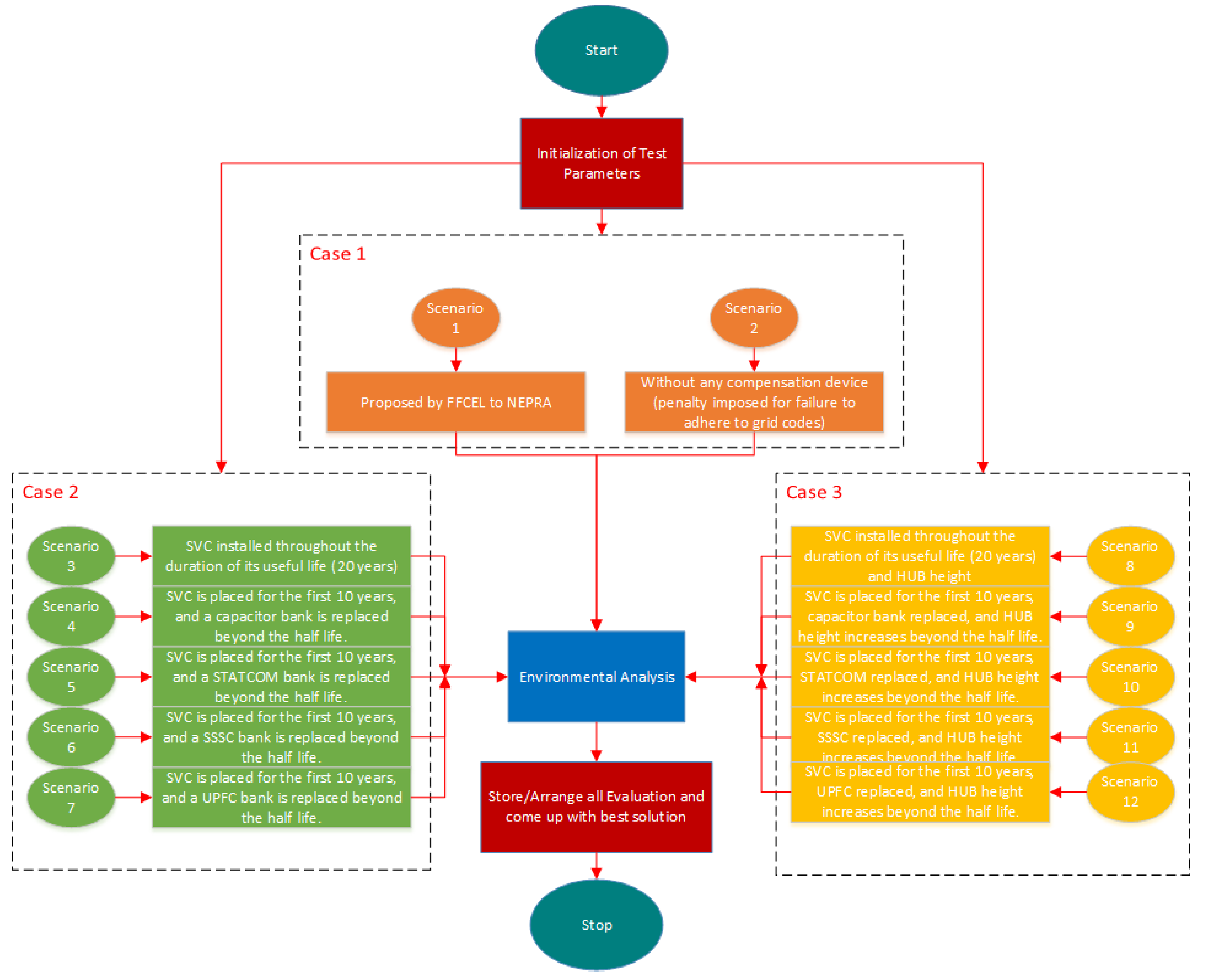
6. Methodology
6.1. Case-1: Base Case Scenarios Assessment
6.2. Case-2: VAR Device-Based Scenario Assessment
6.3. Case-3: VAR Devices and Heightening the Hubs-Based Scenario Assessment
6.4. Environmental Analysis
7. Simulations, Results, and Discussions
7.1. Case-1 Evaluation: Base Case Scenarios Assessment
7.1.1. Case-1, Scenario 1: Proposed by FFCEL to NEPRA
7.1.2. Case-1, Scenario 2: Without any Compensation Device (Penalty Imposed for Failure to Adhere to Grid Codes)
7.2. Case-2 VAR Devices Based Scenario Assessment
7.2.1. Case-2, Scenario 3: SVC Installed throughout the Duration of Its Useful Life (20 Years)
7.2.2. Case-2, Scenario 4: SVC Is Placed for the First 10 Years, and a Capacitor Bank Is Replaced beyond the Half-Life
7.2.3. Case-2, Scenario 5: SVC Is Placed for the First 10 Years, and a STATCOM Bank Is Replaced beyond the Half-Life
7.2.4. Case-2, Scenario 6: SVC Is Placed for the First 10 Years, and an SSSC Bank Is Replaced beyond the Half-Life
7.2.5. Case-2, Scenario 7: SVC Is Placed for the First 10 Years, and a UPFC Bank Is Replaced beyond the Half-Life
7.3. Case-3: VAR Devices and Heightening the Hubs-Based Scenario Assessment
7.3.1. Case-3, Scenario 8: SVC Installed throughout the Duration of Its Useful Life (20 Years), and HUB Height Increases beyond the Half-Life
7.3.2. Case-3, Scenario 9: SVC Is Placed for the First 10 Years, Capacitor Bank Is Replaced, and HUB Height Increases beyond the Half-Life
7.3.3. Case-3, Scenario 10: SVC Is Placed for the First 10 Years, STATCOM Is Replaced, and HUB Height Increases beyond the Half-Life
7.3.4. Case-3, Scenario 11: SVC Is Placed for the First 10 Years, SSSC Is Replaced, and HUB Height Increases beyond the Half-Life
7.3.5. Case-3, Scenario 12: SVC Is Placed for the First 10 Years, UPFC Is Replaced, and HUB Height Increases beyond the Half-Life
7.4. CO2 Reduction and Environmental Assessment
8. Results Validation
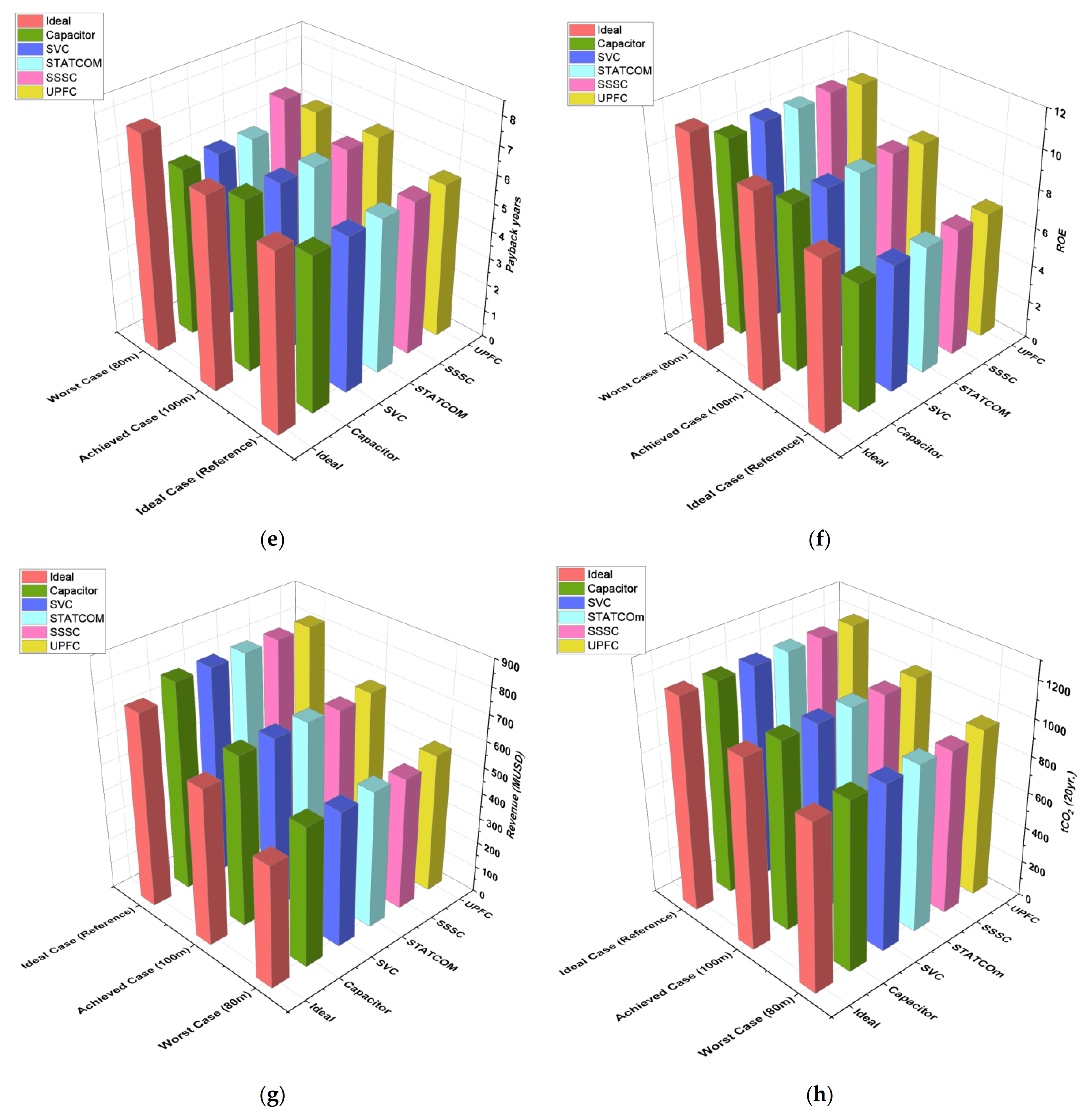
8.1. Comparison between Proposed Cases with a Base Case

| Wind Speed | Devices | Power (MW) | Reactive Power Q (MVAR) | Energy (KWh) |
|---|---|---|---|---|
| 15 (m/s) [21] | Ideal | 48.28 | 2.574 | 139,567,824 |
| Capacitor | 48.25 | −24.33 | 139,481,100 | |
| SVC | 48.25 | −24.33 | 139,481,100 | |
| Statcom | 48.29 | −5.813 | 139,596,732 | |
| SSSC | 48.3 | −1.887 | 139,625,640 | |
| UPFC | 48.31 | −4.109 | 139,654,548 | |
| 11 (m/s) At 100 m HUB height | Ideal | 42.7 | 2.617 | 123,437,160 |
| Capacitor | 42.66 | −24.08 | 123,321,528 | |
| SVC | 42.72 | −24.08 | 123,494,976 | |
| Statcom | 42.77 | −5.283 | 123,639,516 | |
| SSSC | 42.34 | −1.797 | 122,396,472 | |
| UPFC | 42.78 | −3.713 | 123,668,424 | |
| 10 (m/s) At 80 m HUB height | Ideal | 37.63 | 2.749 | 108,780,804 |
| Capacitor | 38.07 | −23.76 | 110,052,756 | |
| SVC | 37.55 | −23.77 | 108,549,540 | |
| Statcom | 37.79 | −4.746 | 109,243,332 | |
| SSSC | 37.16 | −2.007 | 107,422,128 | |
| UPFC | 38.15 | −3.28 | 110,284,020 |
| Scenario #: | P(MW) with Wake at Hub Height = 80 m | P(MW) with Wake at Hub Height = 100 m | V (pu) | Transient F (Hz) | Impedance (Ohms) | PF |
|---|---|---|---|---|---|---|
| Ideal | 37.63 | 42.70 | 0.9704 | 49.36–50.89 | 24.96 | 0.959 |
| Capacitor Bank | 38.07 | 42.66 | 1.028 | 49.55–50.41 | 26.53 | 0.999 |
| SVC | 37.55 | 42.72 | 1.028 | 49.75–50.24 | 24.76 | 0.999 |
| STATCOM | 37.79 | 42.77 | 1.006 | 49.76–50.26 | 24.76 | 0.962 |
| SSSC | 37.16 | 42.34 | 1.004 | 49.67–50.75 | 20.83 | 0.960 |
| UPFC | 38.15 | 42.78 | 1.002 | 49.88–50.17 | 20.83 | 0.962 |
| Wind Speed | Devices | Net Annual GHG Emission Reduction tCO2 | GHG Emission Reduction tCO2 (20 Y) |
|---|---|---|---|
| 15 (ms-1) | Ideal | 58,758.0539 | 1,175,161.078 |
| Capacitor | 58,721.5431 | 1,174,430.862 | |
| SVC | 58,721.5431 | 1,174,430.862 | |
| Statcom | 58,770.22417 | 1,175,404.483 | |
| SSSC | 58,782.39444 | 1,175,647.889 | |
| UPFC | 58,794.56471 | 1,175,891.294 | |
| 10.714 (ms-1) At 100 m HUB height | Ideal | 51,967.04436 | 1,039,340.887 |
| Capacitor | 51,918.36329 | 1,038,367.266 | |
| SVC | 51,991.3849 | 1,039,827.698 | |
| Statcom | 52,052.23624 | 1,041,044.725 | |
| SSSC | 51,528.91471 | 1,030,578.294 | |
| UPFC | 52,064.4065 | 1,041,288.13 | |
| 10.232 (ms-1) At 80 m HUB height | Ideal | 45,796.71848 | 915,934.3697 |
| Capacitor | 46,332.21028 | 926,644.2055 | |
| SVC | 45,699.35634 | 913,987.1268 | |
| Statcom | 45,991.44277 | 919,828.8554 | |
| SSSC | 45,224.71589 | 904,494.3178 | |
| UPFC | 46,429.57242 | 928,591.4484 |
| Wind Speed | Devices | SPP (Year) | ROE (Year) | IRR | Cashflows |
|---|---|---|---|---|---|
| Wind speed 15 (ms-1) | Ideal | 6.44 | 8.860 | 11.617 | 754,310,745.87 |
| Capacitor | 5.639 | 6.714 | 13.335 | 810,062,392.75 | |
| SVC | 5.639 | 6.714 | 13.335 | 810,062,392.75 | |
| Statcom | 5.633 | 6.698 | 13.356 | 811,122,044.39 | |
| SSSC | 5.632 | 6.694 | 13.361 | 811,386,957.30 | |
| UPFC | 5.631 | 6.690 | 13.366 | 811,651,870.21 | |
| Wind speed 10.714 (ms-1) At 100 m HUB height | Ideal | 6.971 | 10.219 | 7.228 | 606,489,342.28 |
| Capacitor | 6.232 | 8.7944 | 9.774 | 661,976,076.25 | |
| SVC | 6.222 | 8.763 | 9.821 | 663,565,553.71 | |
| Statcom | 6.215 | 8.737 | 9.860 | 664,890,118.26 | |
| SSSC | 6.281 | 8.966 | 9.519 | 653,498,863.14 | |
| UPFC | 6.213 | 8.731 | 9.868 | 665,155,031.17 | |
| Wind speed 10.232 (ms-1) At 80 m HUB height | Ideal | 7.862 | 11.416 | 0.652 | 472,178,497.09 |
| Capacitor | 6.1044 | 10.409 | 5.303 | 540,381,050.72 | |
| SVC | 6.1151 | 10.546 | 4.657 | 526,605,579.42 | |
| Statcom | 6.1101 | 10.482 | 4.961 | 532,963,489.25 | |
| SSSC | 7.032 | 10.652 | 4.151 | 516,273,975.94 | |
| UPFC | 6.1028 | 10.388 | 5.399 | 542,500,354.00 |
8.2. Comparative Analysis of Result via Proposed Methodology
| Scenario | USD | |
|---|---|---|
| Scenario 1 | Proposed by FFCEL to NEPRA | - |
| Scenario 2 | Without any compensation device (penalty imposed for failure to adhere to grid codes) | Penalty |
| Scenario 3 | SVC installed throughout the duration of its useful life (20 years) | - |
| Scenario 4 | SVC is placed for the first 10 years, and a capacitor bank is replaced beyond the half-life. | 500,000 |
| Scenario 5 | SVC is placed for the first 10 years, and a STATCOM bank is replaced beyond the half-life. | 2,177,437.5 |
| Scenario 6 | SVC is placed for the first 10 years, and an SSSC bank is replaced beyond the half-life. | 3,299,562.5 |
| Scenario 7 | SVC is placed for the first 10 years, and a UPFC bank is replaced beyond the half-life. | 5,477,000 |
| Scenario 8 | SVC installed throughout the duration of its useful life (20 years) and HUB height | 3,178,735.84 |
| Scenario 9 | SVC is placed for the first 10 years, the capacitor bank is replaced, and HUB height increases beyond the half-life. | 3,678,735.84 |
| Scenario 10 | SVC is placed for the first 10 years, STATCOM is replaced, and HUB height increases beyond the half-life. | 5,356,173.34 |
| Scenario 11 | SVC is placed for the first 10 years, SSSC is replaced, and HUB height increases beyond the half-life. | 6,478,298.34 |
| Scenario 12 | SVC is placed for the first 10 years, UPFC is replaced, and HUB height increases beyond the half-life. | 8,655,735.84 |
| Case | Payback (Year) | SPP (Year) | IRR% | Revenue (End 20 Y) | NPV |
|---|---|---|---|---|---|
| Scenario 1 | 5.4 | 6.259 | 14.45 | 907,017,158.03 | 209,996,976 |
| Scenario 2 | 7.2 | 10.8 | 7.76 | 584,815,234.33 | 60,637,276 |
| Scenario 3 | 6.5 | 9.81 | 10.413 | 677,379,724.04 | 134,946,432 |
| Scenario 4 | 6.5 | 9.81 | 10.234 | 664,404,939.54 | 136,638,432 |
| Scenario 5 | 6.5 | 9.81 | 10.144 | 660,043,295.86 | 135,564,320 |
| Scenario 6 | 6.5 | 9.81 | 10.202 | 653,238,967.53 | 132,700,992 |
| Scenario 7 | 6.5 | 9.81 | 10.094 | 659,411,175.56 | 137,168,144 |
| Scenario 8 | 6.5 | 9.81 | 10.157 | 656,764,248.39 | 144,146,864 |
| Scenario 9 | 6.5 | 9.81 | 10.360 | 674,858,459.04 | 143,954,512 |
| Scenario 10 | 6.5 | 9.81 | 10.324 | 673,821,360.14 | 144,368,560 |
| Scenario 11 | 6.5 | 9.81 | 10.236 | 669,044,194.47 | 142,700,944 |
| Scenario 12 | 6.5 | 9.81 | 10.383 | 682,223,689.44 | 144,419,296 |
| Cases | Power (MW) | Energy (KWh) | ||
|---|---|---|---|---|
| (1–10) Years | (11–20) Years | (1–10) Years | (11–20) Years | |
| Scenario 1 | 49.5 | 49.5 | 143,600,000 | 143,600,000 |
| Scenario 2 | 40.45 | 40.37 | 116,932,860 | 116,932,860 |
| Scenario 3 | 40.37 | 40.37 | 116,701,596 | 116,701,596 |
| Scenario 4 | 40.37 | 40.92 | 116,701,596 | 118,291,536 |
| Scenario 5 | 40.37 | 40.62 | 116,701,596 | 117,424,296 |
| Scenario 6 | 40.37 | 39.94 | 116,701,596 | 115,458,552 |
| Scenario 7 | 40.37 | 41.01 | 116,701,596 | 118,551,708 |
| Scenario 8 | 40.37 | 42.72 | 116,701,596 | 123,494,976 |
| Scenario 9 | 40.37 | 42.66 | 116,701,596 | 123,321,528 |
| Scenario 10 | 40.37 | 42.77 | 116,701,596 | 123,639,516 |
| Scenario 11 | 40.37 | 42.34 | 116,701,596 | 122,396,472 |
| Scenario 12 | 40.37 | 42.78 | 116,701,596 | 123,668,424 |

| Cases | Net Annual GHG Emission Reduction tCO2 | GHG Emission Reduction tCO2 (20 Y) | ||
|---|---|---|---|---|
| (1–10) Years | (11–20) Years | (1–10) Years | (11–20) Years | |
| Scenario 1 | 60,455.6 | 60,455.6 | 604,556 | 604,556 |
| Scenario 2 | 49,228.73 | 49,228.73 | 492,287.3 | 492,287.3 |
| Scenario 3 | 49,131.37 | 49,131.37 | 491,313.7 | 491,313.7 |
| Scenario 4 | 49,131.37 | 49,800.74 | 491,313.7 | 498,007.4 |
| Scenario 5 | 49,131.37 | 49,435.63 | 491,313.7 | 494,356.3 |
| Scenario 6 | 49,131.37 | 48,608.05 | 491,313.7 | 486,080.5 |
| Scenario 7 | 49,131.37 | 49,910.27 | 491,313.7 | 499,102.7 |
| Scenario 8 | 49,131.37 | 51,991.38 | 491,313.7 | 519,913.8 |
| Scenario 9 | 49,131.37 | 51,918.36 | 491,313.7 | 519,183.6 |
| Scenario 10 | 49,131.37 | 52,052.24 | 491,313.7 | 520,522.4 |
| Scenario 11 | 49,131.37 | 51,528.91 | 491,313.7 | 515,289.1 |
| Scenario 12 | 49,131.37 | 52,064.41 | 491,313.7 | 520,644.1 |
9. Conclusions
Author Contributions
Funding
Institutional Review Board Statement
Informed Consent Statement
Data Availability Statement
Acknowledgments
Conflicts of Interest
Appendix A

References
- Al-Ghussain, L.; Samu, R.; Taylan, O.; Fahrioglu, M. Techno-Economic Comparative Analysis of Renewable Energy Systems: Case Study in Zimbabwe. Inventions 2020, 5, 27. [Google Scholar] [CrossRef]
- Abdin, Z.; Mérida, W. Hybrid energy systems for off-grid power supply and hydrogen production based on renewable energy: A techno-economic analysis. Energy Convers. Manag. 2019, 196, 1068–1079. [Google Scholar] [CrossRef]
- Yan, J.; Ouyang, T. Advanced wind power prediction based on data-driven error correction. Energy Convers. Manag. 2019, 180, 302–311. [Google Scholar] [CrossRef]
- Renewable Capacity Highlights Renewable Generation Capacity by Energy Source. Available online: www.irena.org/publications (accessed on 15 September 2021).
- Rahimi, E.; Rabiee, A.; Aghaei, J.; Muttaqi, K.M.; Esmaeel Nezhad, A. On the management of wind power intermittency. Renew. Sustain. Energy Rev. 2013, 28, 643–653. [Google Scholar] [CrossRef] [Green Version]
- Rona, B.; Güler, Ö. Power system integration of wind farms and analysis of grid code requirements. Renew. Sustain. Energy Rev. 2015, 49, 100–107. [Google Scholar] [CrossRef]
- Wind Energy Comes of Age-Paul Gipe-Google Books. Available online: https://books.google.com.pk/books?hl=en&lr=&id=8itBNxBL4igC&oi=fnd&pg=PR13&ots=HPrxBnHxgT&sig=SWeCcG6C4U7jvrzj1Ql1_k0AT3w&redir_esc=y#v=onepage&q&f=false (accessed on 17 September 2021).
- Manwell, J.F.; McGowan, J.G.; Rogers, A.L. Wind Energy Explained: Theory, Design and Application. Available online: https://books.google.com.pk/books?hl=en&lr=&id=roaTx_Of0vAC&oi=fnd&pg=PR5&ots=O4TzVvfMY9&sig=A0OawDmM59LN8AIE9g4kV9KywMU&redir_esc=y#v=onepage&q&f=false (accessed on 17 September 2021).
- Global Wind Atlas. Available online: https://globalwindatlas.info/ (accessed on 17 September 2021).
- Adelaja, A.; McKeown, C.; Calnin, B.; Hailu, Y. Assessing offshore wind potential. Energy Policy 2012, 42, 191–200. [Google Scholar] [CrossRef]
- Komusanac, I.; Fraile, D.; Brindley, G. Wind energy in Europe in 2019—Trends and statistics. Available online: https://windeurope.org/intelligence-platform/product/wind-energy-in-europe-in-2019-trends-and-statistics/ (accessed on 17 September 2021).
- Ramírez, L.; Fraile, D.; Brindley, G. Offshore wind in Europe: Key trends and statistics 2019. 2020. Available online: http://imis.nioz.nl/imis.php?module=ref&refid=321467 (accessed on 17 September 2021).
- Huang, Y.W.; Kittner, N.; Kammen, D.M. ASEAN grid flexibility: Preparedness for grid integration of renewable energy. Energy Policy 2019, 128, 711–726. [Google Scholar] [CrossRef]
- MF, H.; SK, L.; JO, D. Wind farm power optimization through wake steering. Proc. Natl. Acad. Sci. USA 2019, 116, 14495–14500. [Google Scholar] [CrossRef] [Green Version]
- Topham, E.; McMillan, D. Sustainable decommissioning of an offshore wind farm. Renew. Energy 2017, 102, 470–480. [Google Scholar] [CrossRef] [Green Version]
- Staffell, I.; Green, R. How does wind farm performance decline with age? Renew. Energy 2014, 66, 775–786. [Google Scholar] [CrossRef] [Green Version]
- Castro-Santos, L.; Vizoso, A.F.; Camacho, E.M.; Piegiari, L. Costs and feasibility of repowering wind farms. Energy Sources Part B Econ. Plan. Policy 2016, 11, 974–981. [Google Scholar] [CrossRef]
- González-Longatt, F.; Wall, P.P.; Terzija, V. Wake effect in wind farm performance: Steady-state and dynamic behavior. Renew. Energy 2012, 39, 329–338. [Google Scholar] [CrossRef]
- Lundquist, J.K.; DuVivier, K.K.; Kaffine, D.; Tomaszewski, J.M. Costs and consequences of wind turbine wake effects arising from uncoordinated wind energy development. Nat. Energy 2018, 4, 26–34. [Google Scholar] [CrossRef]
- Vasel-Be-Hagh, A.; Archer, C.L. Wind farm hub height optimization. Appl. Energy 2017, 195, 905–921. [Google Scholar] [CrossRef]
- Abbas, S.R.; Kazmi, S.A.A.; Naqvi, M.; Javed, A.; Naqvi, S.R.; Ullah, K.; Khan, T.U.R.; Shin, D.R. Impact Analysis of Large-Scale Wind Farms Integration in Weak Transmission Grid from Technical. Energies 2020, 13, 5513. [Google Scholar] [CrossRef]
- Ouyang, J.; Li, M.; Zhang, Z.; Tang, T. Multi-timescale active and reactive power-coordinated control of large-scale wind integrated power system for severe wind speed fluctuation. IEEE Access 2019, 7, 51201–51210. [Google Scholar] [CrossRef]
- Ameur, A.; Berrada, A.; Loudiyi, K.; Aggour, M. Analysis of renewable energy integration into the transmission network. Electr. J. 2019, 32, 106676. [Google Scholar] [CrossRef]
- Chompoo-Inwai, C.; Yingvivatanapong, C.; Methaprayoon, K.; Lee, W.J. Closure to discussion of Reactive compensation techniques to improve the ride-through capability of wind turbine during disturbance. IEEE Trans. Ind. Appl. 2005, 41, 1484. [Google Scholar] [CrossRef]
- imen, L.; Djamel, L.; Zohra, M.; Selwa, F. Influence of the wind farm integration on load flow and voltage in electrical power system. Int. J. Hydrogen Energy 2016, 41, 12603–12617. [Google Scholar] [CrossRef]
- Kraiczy, M.; Wang, H.; Schmidt, S.; Wirtz, F.; Braun, M. Reactive power management at the transmission-distribution interface with the support of distributed generators—A grid planning approach. IET Gener. Transm. Distrib. 2018, 12, 5949–5955. [Google Scholar] [CrossRef]
- Prasai, A.; Sastry, J.; Divan, D.M. Dynamic capacitor (D-CAP): An integrated approach to reactive and harmonic compensation. IEEE Trans. Ind. Appl. 2010, 46, 2518–2525. [Google Scholar] [CrossRef]
- Ouyang, J.; Tang, T.; Yao, J.; Li, M. Active Voltage Control for DFIG-based Wind Farm Integrated Power System by Coordinating Active and Reactive Powers under Wind Speed Variations. IEEE Trans. Energy Convers. 2019, 34, 1504–1511. [Google Scholar] [CrossRef]
- She, X.; Huang, A.Q.; Wang, F.; Burgos, R. Wind energy system with integrated functions of active power transfer, reactive power compensation, and voltage conversion. IEEE Trans. Ind. Electron. 2013, 60, 4512–4524. [Google Scholar] [CrossRef]
- Chen, B.; Fei, W.; Tian, C.; Yuan, J. Research on an Improved Hybrid Unified Power Flow Controller. IEEE Trans. Ind. Appl. 2018, 54, 5649–5660. [Google Scholar] [CrossRef]
- Jowder, F.A.L. Influence of mode of operation of the SSSC on the small disturbance and transient stability of a radial power system. IEEE Trans. Power Syst. 2005, 20, 935–942. [Google Scholar] [CrossRef]
- Mahela, O.P.; Shaik, A.G. Comprehensive overview of grid interfaced wind energy generation systems. Renew. Sustain. Energy Rev. 2016, 57, 260–281. [Google Scholar] [CrossRef]
- Howard, D.F.; Jiaqi, L.; Harley, R.G. Short-circuit modeling of DFIGs with uninterrupted control. IEEE J. Emerg. Sel. Top. Power Electron. 2014, 2, 47–57. [Google Scholar] [CrossRef]
- Liu, M.; Pan, W.; Quan, R.; Li, H.; Liu, T.; Yang, G. A Short-Circuit Calculation Method for DFIG-Based Wind Farms. IEEE Access 2018, 6, 52793–52800. [Google Scholar] [CrossRef]
- Chrysochoidis-Antsos, N.; Escudé, M.R.; van Wijk, A.J.M. Technical potential of on-site wind powered hydrogen producing refuelling stations in the Netherlands. Int. J. Hydrogen Energy 2020, 45, 25096–25108. [Google Scholar] [CrossRef]
- Mendes, P.R.C.; Isorna, L.V.; Bordons, C.; Normey-Rico, J.E. Energy management of an experimental microgrid coupled to a V2G system. J. Power Sources 2016, 327, 702–713. [Google Scholar] [CrossRef]
- Shehzad, M.F.; Abdelghany, M.B.; Liuzza, D.; Mariani, V.; Glielmo, L. Mixed Logic Dynamic Models for MPC Control of Wind Farm Hydrogen-Based Storage Systems. Inventions 2019, 4, 57. [Google Scholar] [CrossRef] [Green Version]
- Quarton, C.J.; Tlili, O.; Welder, L.; Mansilla, C.; Blanco, H.; Heinrichs, H.; Leaver, J.; Samsatli, N.J.; Lucchese, P.; Robinius, M.; et al. The curious case of the conflicting roles of hydrogen in global energy scenarios. Sustain. Energy Fuels 2019, 4, 80–95. [Google Scholar] [CrossRef] [Green Version]
- Apostolou, D.; Enevoldsen, P. The past, present and potential of hydrogen as a multifunctional storage application for wind power. Renew. Sustain. Energy Rev. 2019, 112, 917–929. [Google Scholar] [CrossRef]
- Trifkovic, M.; Sheikhzadeh, M.; Nigim, K.; Daoutidis, P. Modeling and control of a renewable hybrid energy system with hydrogen storage. IEEE Trans. Control Syst. Technol. 2014, 22, 169–179. [Google Scholar] [CrossRef]
- Castro-Santos, L.; Filgueira-Vizoso, A.; Carral-Couce, L.; Formoso, J.Á.F. Economic feasibility of floating offshore wind farms. Energy 2016, 112, 868–882. [Google Scholar] [CrossRef]
- Myhr, A.; Bjerkseter, C.; Ågotnes, A.; Nygaard, T.A. Levelised cost of energy for offshore floating wind turbines in a life cycle perspective. Renew. Energy 2014, 66, 714–728. [Google Scholar] [CrossRef] [Green Version]
- De Prada Gil, M.; Domínguez-García, J.L.; Díaz-González, F.; Aragüés-Peñalba, M.; Gomis-Bellmunt, O. Feasibility analysis of offshore wind power plants with DC collectiongrid. Renew. Energy 2015, 78, 467–477. [Google Scholar] [CrossRef] [Green Version]
- Kaldellis, J.K. Stand-Alone and Hybrid Wind Energy Systems: Technology, Energy Storage and Applications; Woodhead Publishing: Sawston, UK, 2010; Volume 554. [Google Scholar]
- Ioannou, A.; Angus, A.; Brennan, F. Parametric CAPEX, OPEX, and LCOE expressions for offshore wind farms based on global deployment parameters. Energy Sources Part B Econ. Plan. Policy 2018, 13, 281–290. [Google Scholar] [CrossRef] [Green Version]
- Projected Costs of Generating Electricity 2015—Analysis—IEA. Available online: https://www.iea.org/reports/projected-costs-of-generating-electricity-2015 (accessed on 13 September 2021).
- Bölük, G.; Mert, M. Fossil & renewable energy consumption, GHGs (greenhouse gases) and economic growth: Evidence from a panel of EU (European Union) countries. Energy 2014, 74, 439–446. [Google Scholar] [CrossRef]
- Shayanmehr, S.; Henneberry, S.R.; Sabouni, M.S.; Foroushani, N.S. Drought, Climate Change, and Dryland Wheat Yield Response: An Econometric Approach. Int. J. Environ. Res. Public Health 2020, 17, 5264. [Google Scholar] [CrossRef]
- Irtija, N.; Sangoleye, F.; Tsiropoulou, E.E. Contract-theoretic demand response management in smart grid systems. IEEE Access 2020, 8, 184976–184987. [Google Scholar] [CrossRef]
- Wei, W.; Hao, S.; Yao, M.; Chen, W.; Wang, S.; Wang, Z.; Wang, Y.; Zhang, P. Unbalanced economic benefits and the electricity-related carbon emissions embodied in China’s interprovincial trade. J. Environ. Manage. 2020, 263, 110390. [Google Scholar] [CrossRef]
- Georgatzi, V.V.; Stamboulis, Y.; Vetsikas, A. Examining the determinants of CO2 emissions caused by the transport sector: Empirical evidence from 12 European countries. Econ. Anal. Policy 2020, 65, 11–20. [Google Scholar] [CrossRef]
- Kumar, I.; Tyner, W.E.; Sinha, K.C. Input–output life cycle environmental assessment of greenhouse gas emissions from utility scale wind energy in the United States. Energy Policy 2016, 89, 294–301. [Google Scholar] [CrossRef]
- Vargas, A.V.; Zenón, E.; Oswald, U.; Islas, J.M.; Güereca, L.P.; Manzini, F.L. Life cycle assessment: A case study of two wind turbines used in Mexico. Appl. Therm. Eng. 2015, 75, 1210–1216. [Google Scholar] [CrossRef]
- Gomaa, M.R.; Rezk, H.; Mustafa, R.J.; Al-Dhaifallah, M. Evaluating the Environmental Impacts and Energy Performance of a Wind Farm System Utilizing the Life-Cycle Assessment Method: A Practical Case Study. Energies 2019, 12, 3263. [Google Scholar] [CrossRef] [Green Version]
- Oebels, K.B.; Pacca, S. Life cycle assessment of an onshore wind farm located at the northeastern coast of Brazil. Renew. Energy 2013, 53, 60–70. [Google Scholar] [CrossRef]
- Demir, N.; Taşkin, A. Life cycle assessment of wind turbines in Pınarbaşı-Kayseri. J. Clean. Prod. 2013, 54, 253–263. [Google Scholar] [CrossRef]
- Hondo, H. Life cycle GHG emission analysis of power generation systems: Japanese case. Energy 2005, 30, 2042–2056. [Google Scholar] [CrossRef]
- Al-Behadili, S.H.; El-Osta, W.B. Life Cycle Assessment of Dernah (Libya) wind farm. Renew. Energy 2015, 83, 1227–1233. [Google Scholar] [CrossRef]
- Hadžić, N.; Kozmar, H.; Tomić, M. Offshore renewable energy in the Adriatic Sea with respect to the Croatian 2020 energy strategy. Renew. Sustain. Energy Rev. 2014, 40, 597–607. [Google Scholar] [CrossRef]
- Mahfouz, M.M.; El-Sayed, M.A.H. Static synchronous compensator sizing for enhancement of fault ride-through capability and voltage stabilisation of fixed speed wind farms. IET Renew. Power Gener. 2014, 8, 1–9. [Google Scholar] [CrossRef]
- 2010 to 2015 Government Policy: Low Carbon Technologies—GOV.UK. Available online: https://www.gov.uk/government/publications/2010-to-2015-government-policy-low-carbon-technologies/2010-to-2015-government-policy-low-carbon-technologies#appendix-4-offshore-wind (accessed on 20 September 2021).
- NTDC, MERIT ORDER Based on Revised Fuel Prices, National Transmission and Dispatch Company Limited, Pakistan. 22 January, (2021). Available online: https://ntdc.gov.pk/ntdc/public/uploads/services/meritorder/2021/January/MERIT%20ORDER%20WEF%2021%20JAN%202021.pdf (accessed on 8 September 2021).
- Ministry of Finance, Government of Pakistan. Economic Survey of Pakistan; 2021. Available online: https://www.finance.gov.pk/survey_2021.html (accessed on 8 September 2021).
- Shaikh, F.; Ji, Q.; Fan, Y. The diagnosis of an electricity crisis and alternative energy development in Pakistan. Renew. Sustain. Energy Rev. 2015, 52, 1172–1185. [Google Scholar] [CrossRef]
- Nosratabadi, S.M.; Hooshmand, R.A.; Gholipour, E. Stochastic profit-based scheduling of industrial virtual power plant using the best demand response strategy. Appl. Energy 2016, 164, 590–606. [Google Scholar] [CrossRef]
- Hulio, Z.H.; Jiang, W.; Rehman, S. Technical and economic assessment of wind power potential of Nooriabad, Pakistan. Energy. Sustain. Soc. 2017, 7, 1–14. [Google Scholar] [CrossRef]
- Internal Rate of Return (IRR) Definition & Formula. Available online: https://www.investopedia.com/terms/i/irr.asp (accessed on 4 October 2021).
- Cai, L.J.; Erlich, I.; Stamtsis, G.C. Optimal choice and allocation of FACTS devices in deregulated electricity market using genetic algorithms. 2004 IEEE PES Power Syst. Conf. Expo. 2004, 1, 201–207. [Google Scholar] [CrossRef]
- Helmy, W.; Abbas, M.A.E. Optimal sizing of capacitor-bank types in the low voltage distribution networks using JAYA optimization. In Proceedings of the 2018 9th International Renewable Energy Congress (IREC), Hammamet, Tunisia, 20–22 March 2018; pp. 1–5. [Google Scholar] [CrossRef]
- Ghiasi, M. Technical and economic evaluation of power quality performance using FACTS devices considering renewable micro-grids. Renew. Energy Focus 2019, 29, 49–62. [Google Scholar] [CrossRef]
- Himri, Y.; Rehman, S.; Draoui, B.; Himri, S. Wind power potential assessment for three locations in Algeria. Renew. Sustain. Energy Rev. 2008, 12, 2495–2504. [Google Scholar] [CrossRef]
- Clean Energy Project Analysis Third Edition RETScreen ® Engineering & Cases Textbook. Available online: https://nrcaniets.blob.core.windows.net/iets/RETScreen_Engineering_e-textbook.pdf. (accessed on 17 September 2021).
- Syed, A.H.; Javed, A.; Asim Feroz, R.M.; Calhoun, R. Partial repowering analysis of a wind farm by turbine hub height variation to mitigate neighboring wind farm wake interference using mesoscale simulations. Appl. Energy 2020, 268, 115050. [Google Scholar] [CrossRef]
- Solid, M.; Power, W.; Sir, D.; Secretariat, P.; Division, C.; Secretariat, C.; Secretariat, P. National Electric Power Regulatory Authority Islamic Republic of Pakistan Determination of the Authority in the matter of Upfront Generation Tariff for. 2018, 5–7. Available online: https://nepra.org.pk/tariff/Tariff/IPPs/FFC%20Energy%20Ltd/TRF-156%20FFC%20EL%20COD%2010-11-2014%2014119-21.PDF. (accessed on 17 September 2021).
- Government of Pakistan Ministry of Planning, Development and Special Initiatives Pakistan Bureau pf Statistics Press Release on Consumer Price Index (CPI) Inflation for the Month Analysis of Consumer Price Index (CPI) Base Year (2015-16) 2. 2020. Available online: http://www.pbs.gov.pk (accessed on 5 October 2021).
- State Bank of Pakistan. Available online: https://www.sbp.org.pk/smefd/circulars/2016/C3.htm (accessed on 5 October 2021).
- National Electric Power Regulatory Authority Islamic Republic of Pakistan Registrar. Available online: www.nepra.org.pk (accessed on 5 October 2021).
- Rules, P.; Electric, N.; Act, E.P. National Electric Power Regulatory Authority Schedule. Cell 2002, 385, 3–6. Available online: https://nepra.org.pk/Legislation/2-Rules/2.4%20NEPRA%20(Fees)%20Rules,%202002/NEPRA%20Fee%20Rules%20along%20with%20amendment%202020.pdf (accessed on 17 September 2021).
- NEPRA Grid Code Addendum No. 1 for Grid Integration of Wind Power Plants, April 2010. Available online: https://nepra.org.pk/Standards/Codes/NTDC-GRID%20CODE%20ADDENDUM%20NO%20I.PDF (accessed on 5 October 2021).
- Saqib, M.A.; Saleem, A.Z. Power-quality issues and the need for reactive-power compensation in the grid integration of wind power. Renew. Sustain. Energy Rev. 2015, 43, 51–64. [Google Scholar] [CrossRef]


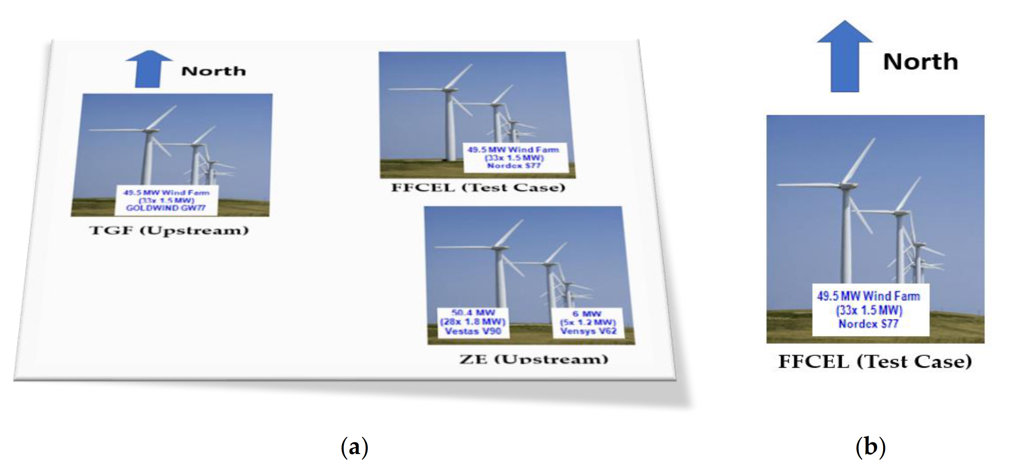
| Data | TGF (Upstream) | ZE (Upstream) | FFCEL (Test Case) |
|---|---|---|---|
| Date of Operation | November 2014 | July 2013 | May 2013 |
| Turbines model | Goldwind GW771500 | Vestas and Vensys-62 | Nordex-S77 |
| Turbine capacity (MW) | 1.5 | Vestas = 1.8; Vensys-62 = 1.2 | 1.5 |
| Total number of wind turbines | 33 | 28 × Vestas; 5 × Vesys-62 | 33 |
| WF capacity (MW) | 49.5 | 56.4 | 49.5 |
| Type of Generator | DFIG | DFIG | DFIG |
| Generators output voltage (V) | 660 | 660 | 660 |
| Parameters | Grid Codes |
|---|---|
| Reactive Power Control | At PCC, the wind farm should manage reactive power to keep the power factor within the required range (0.95 lagging to 0.95 leading over the whole range of plant operation). |
| Harmonics | Wind turbines with power converters produce harmonics. Voltage and current harmonics up to 50 times the essential power frequency may be defined according to IEC61400-21. According to widely accepted standards, the PCC’s total harmonic distortion (THD) from these harmonics must be less than 5%, and there ought to be no resonance at odd-frequency harmonics. |
| Frequency | For the provided system frequency range, the wind farm must be able to operate constantly within 49.5 to 50.5 Hz |
| Resonance | Odd harmonics are harmful to the power system; hence, there should be no odd harmonics. |
| Voltage Control | The WF should be able to produce available power while maintaining a tolerable voltage at the grid-connection point (PCC) (75% of nominal voltage). |
Publisher’s Note: MDPI stays neutral with regard to jurisdictional claims in published maps and institutional affiliations. |
© 2022 by the authors. Licensee MDPI, Basel, Switzerland. This article is an open access article distributed under the terms and conditions of the Creative Commons Attribution (CC BY) license (https://creativecommons.org/licenses/by/4.0/).
Share and Cite
Butt, R.Z.; Kazmi, S.A.A.; Alghassab, M.; Khan, Z.A.; Altamimi, A.; Imran, M.; Alruwaili, F.F. Techno-Economic and Environmental Impact Analysis of Large-Scale Wind Farms Integration in Weak Transmission Grid from Mid-Career Repowering Perspective. Sustainability 2022, 14, 2507. https://doi.org/10.3390/su14052507
Butt RZ, Kazmi SAA, Alghassab M, Khan ZA, Altamimi A, Imran M, Alruwaili FF. Techno-Economic and Environmental Impact Analysis of Large-Scale Wind Farms Integration in Weak Transmission Grid from Mid-Career Repowering Perspective. Sustainability. 2022; 14(5):2507. https://doi.org/10.3390/su14052507
Chicago/Turabian StyleButt, Rohan Zafar, Syed Ali Abbas Kazmi, Mohammed Alghassab, Zafar A. Khan, Abdullah Altamimi, Muhammad Imran, and Fahad F. Alruwaili. 2022. "Techno-Economic and Environmental Impact Analysis of Large-Scale Wind Farms Integration in Weak Transmission Grid from Mid-Career Repowering Perspective" Sustainability 14, no. 5: 2507. https://doi.org/10.3390/su14052507
APA StyleButt, R. Z., Kazmi, S. A. A., Alghassab, M., Khan, Z. A., Altamimi, A., Imran, M., & Alruwaili, F. F. (2022). Techno-Economic and Environmental Impact Analysis of Large-Scale Wind Farms Integration in Weak Transmission Grid from Mid-Career Repowering Perspective. Sustainability, 14(5), 2507. https://doi.org/10.3390/su14052507