
ESMA-OPF: Enhanced Slime Mould Algorithm for Solving Optimal Power Flow Problem


Abstract
:1. Introduction
2. Problem Formulation
2.1. Cost Model of TPGs
2.2. Direct Power Cost of SPG and WPGs
2.3. Cost Assessment for Uncertain Wind Power Output
2.4. Cost Assessment for Uncertain Solar PV Power
2.5. Emissions and Carbon Tax
2.6. Objective Functions of the OPF
2.6.1. Equality Constraints
2.6.2. Inequality Constraints
- 1.
- Constraints of Generators:
- 2.
- Security constraints:
- 3.
- TPGs Ramp Rate Constraints:
3. Stochastic Solar Power, Wind Power, and Models of Uncertainty
3.1. Models of Solar and Wind Powers
3.2. Probability Calculation of Wind Power
3.3. Over/Underestimation Cost of Solar Power
4. Optimization Algorithm
4.1. Original SMA
4.1.1. Food Approach
4.1.2. Wrap Food
4.1.3. Grabble Food
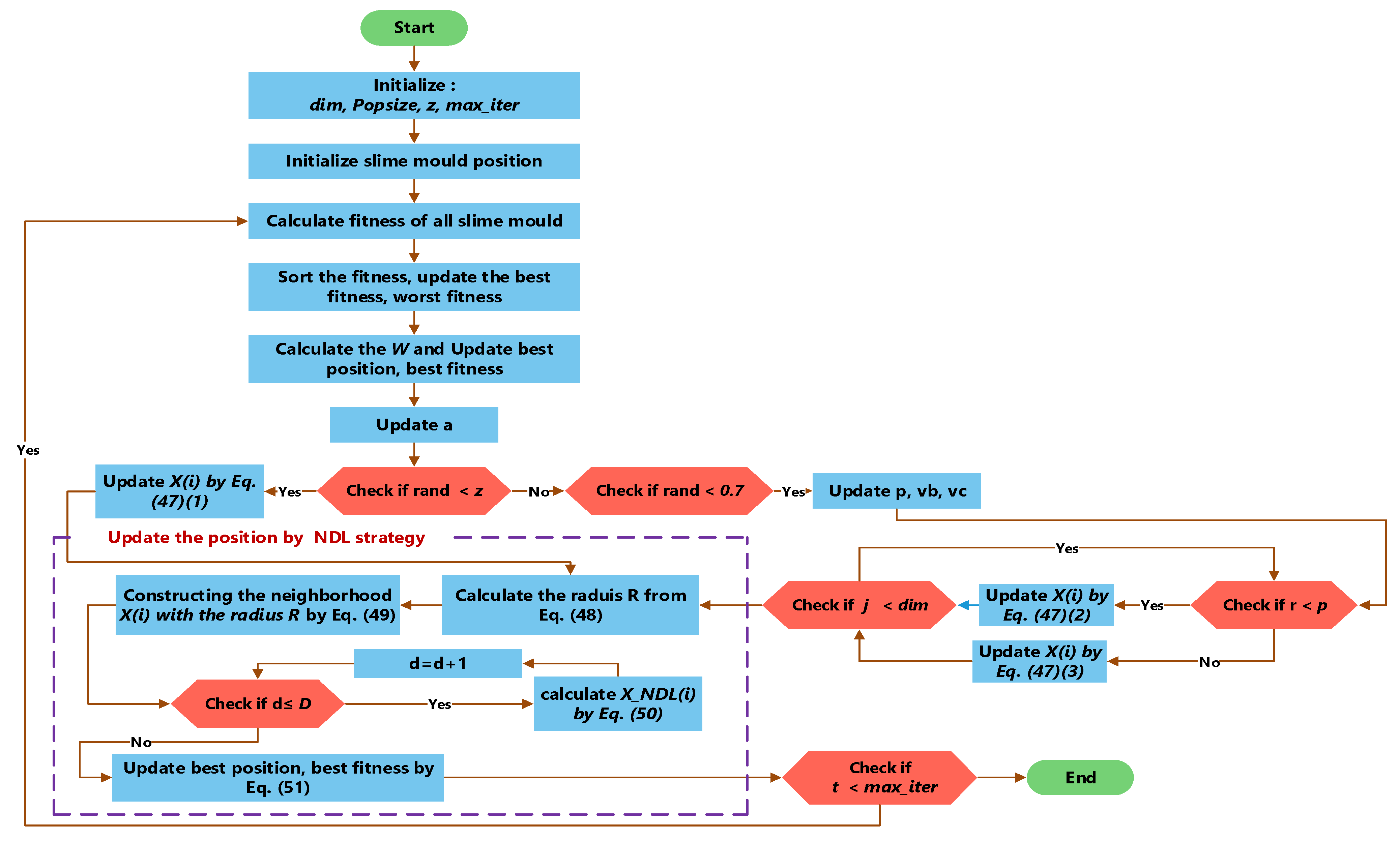
4.2. Proposed ESMA
5. Results
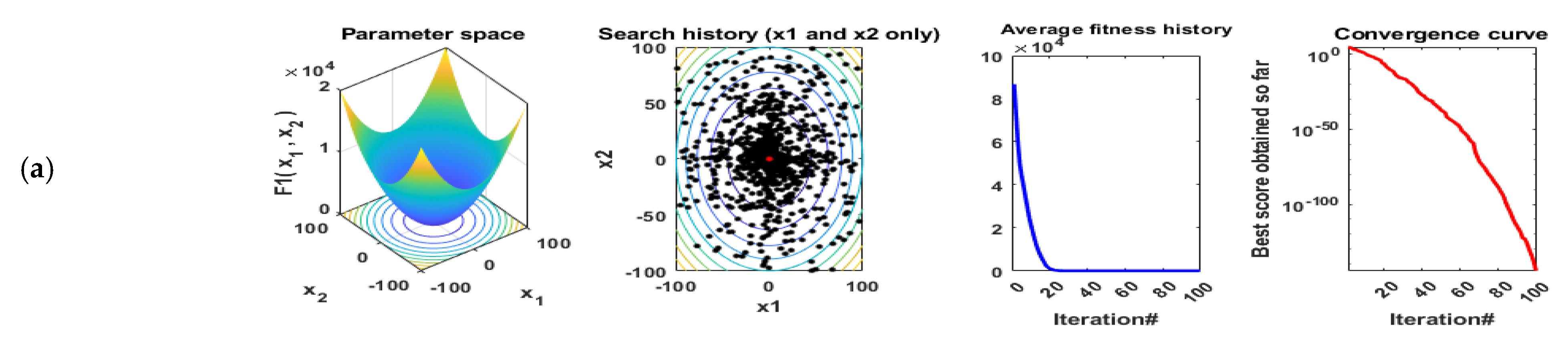
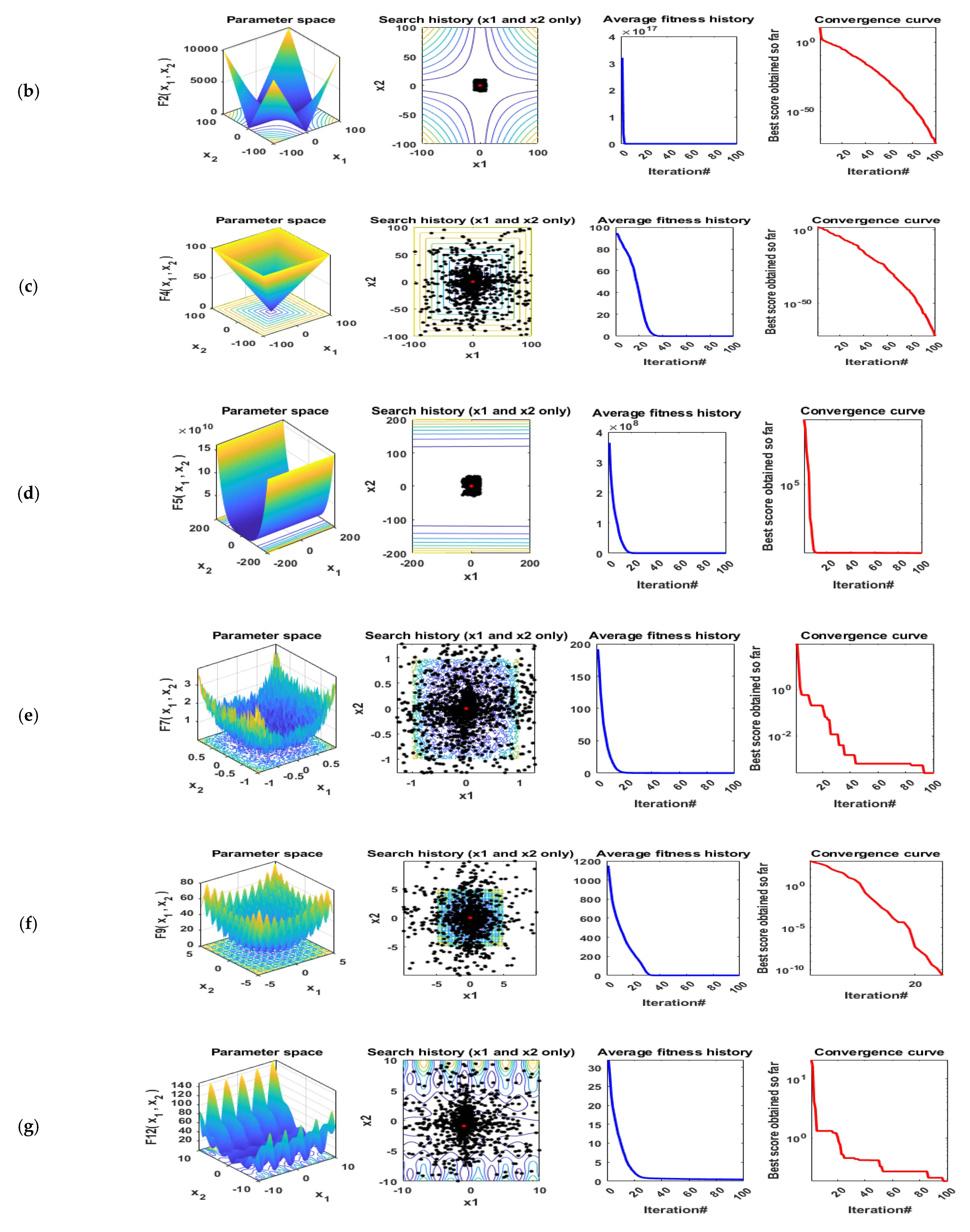
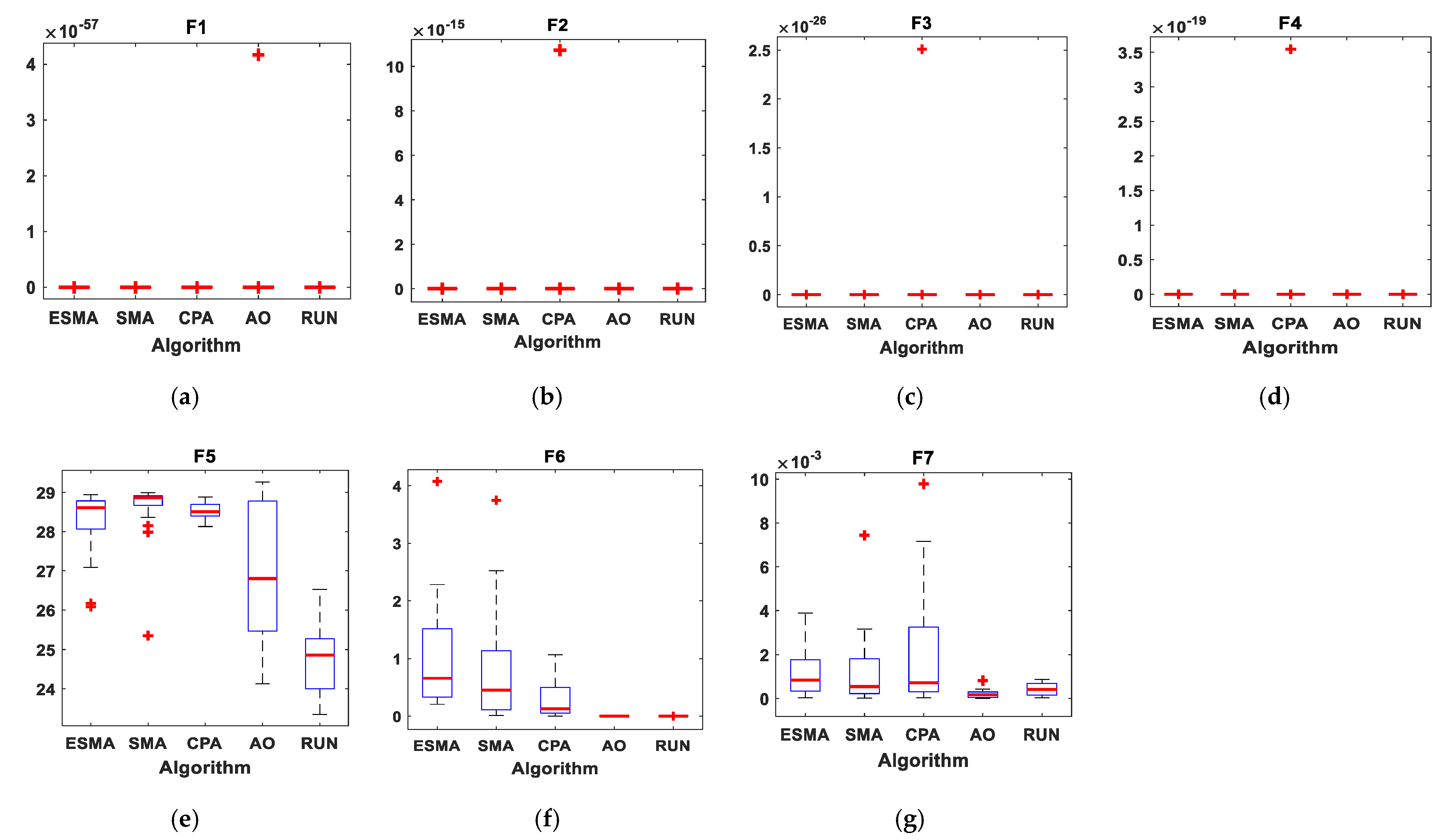
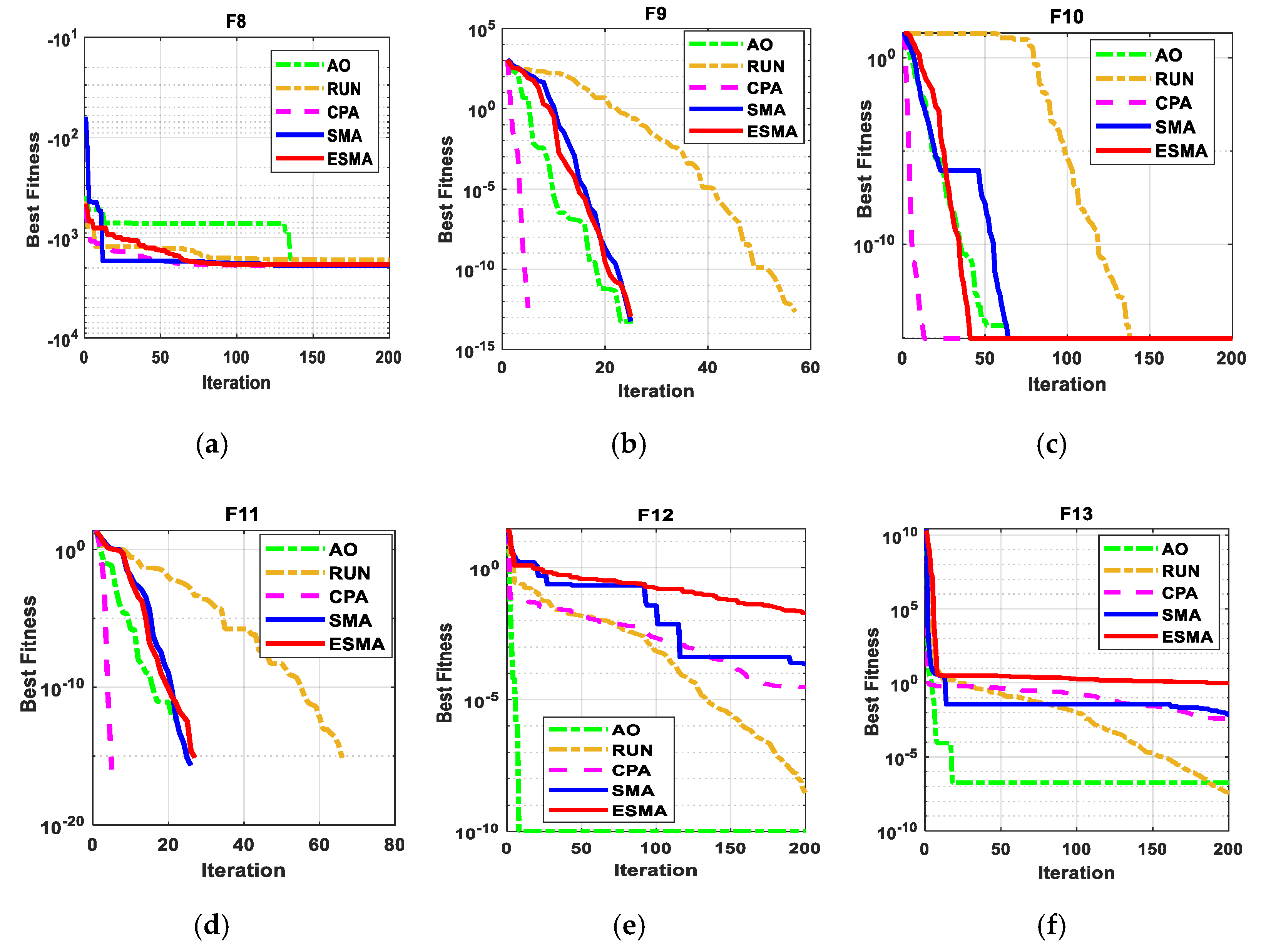
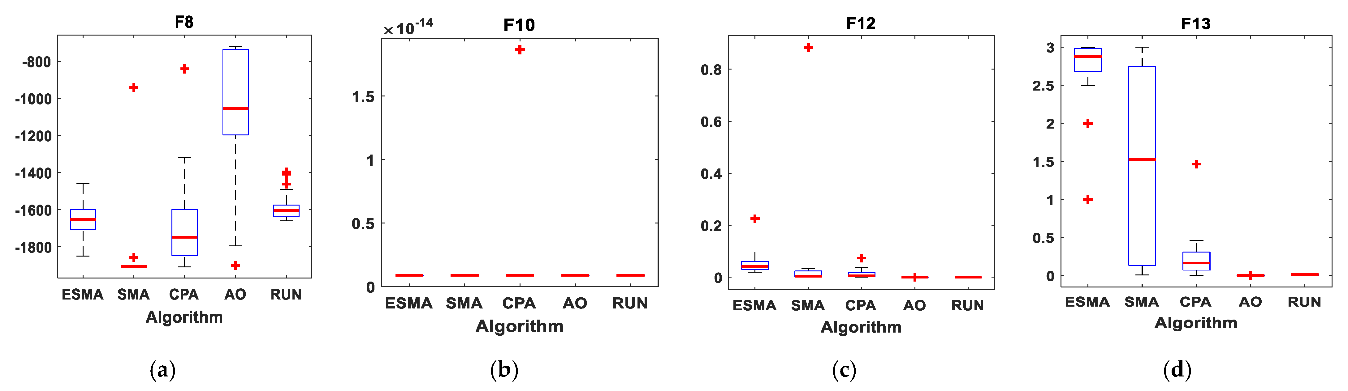
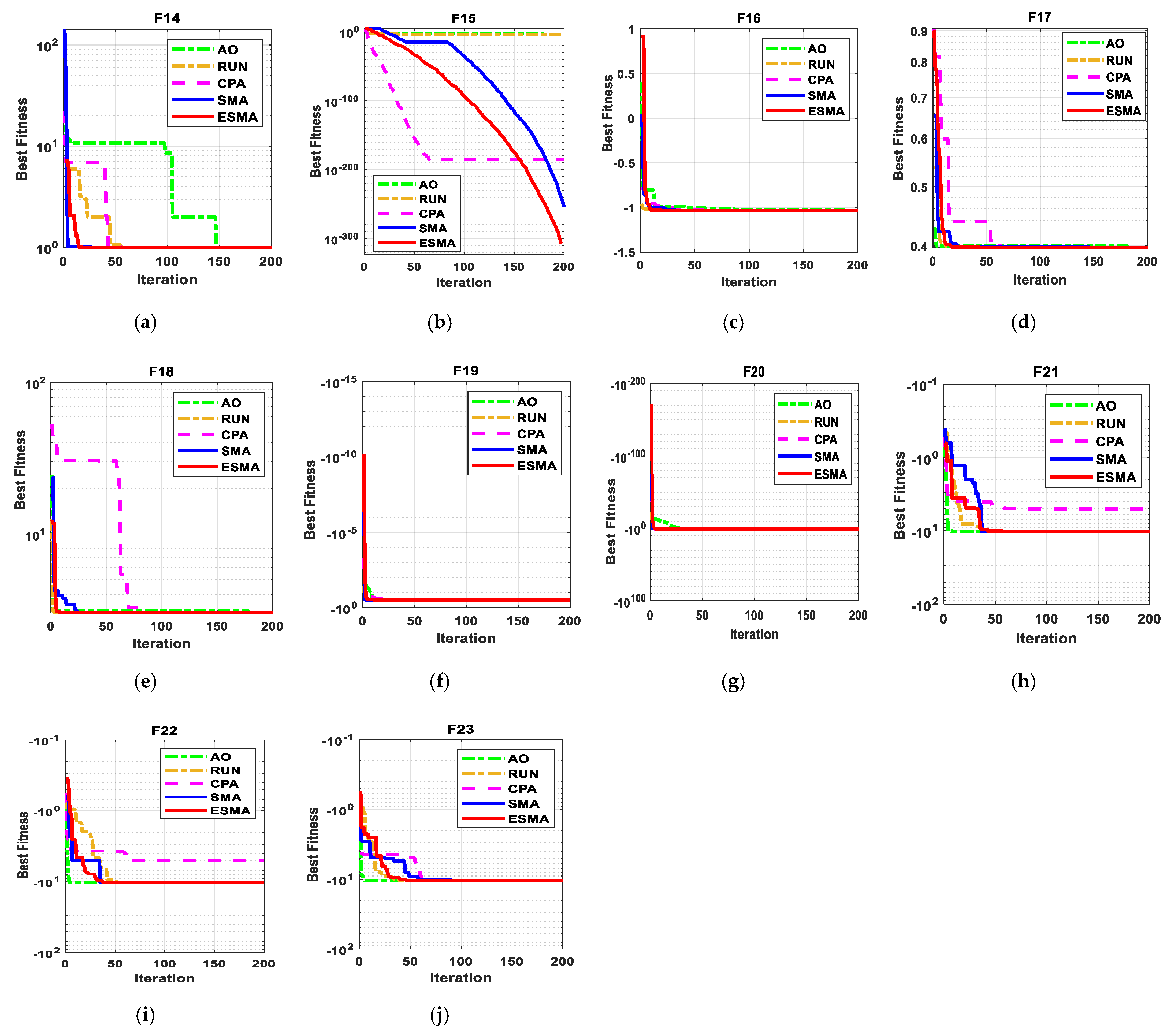
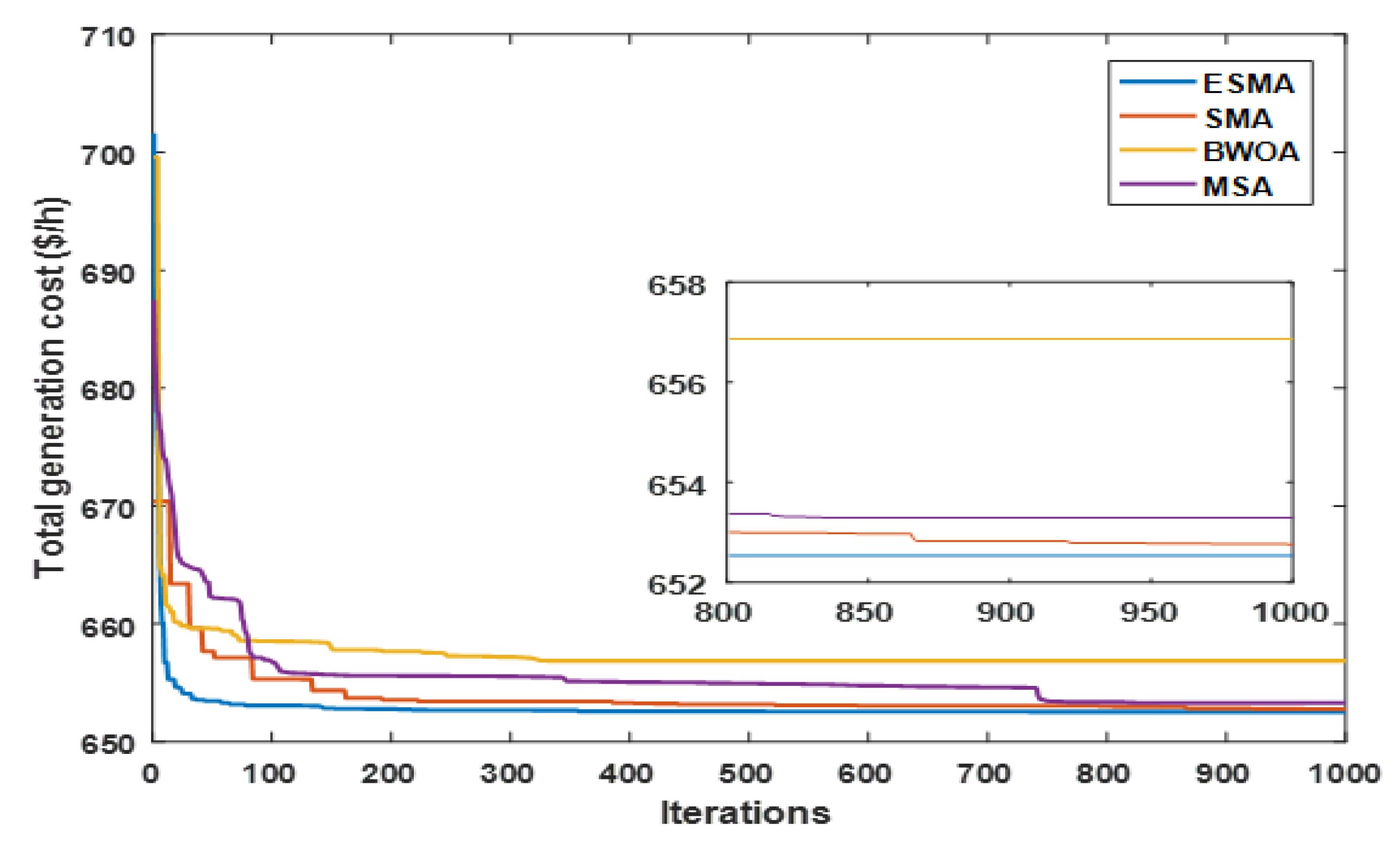
5.1. Performance of the Proposed ESMA Algorithm
5.2. Real-World Application
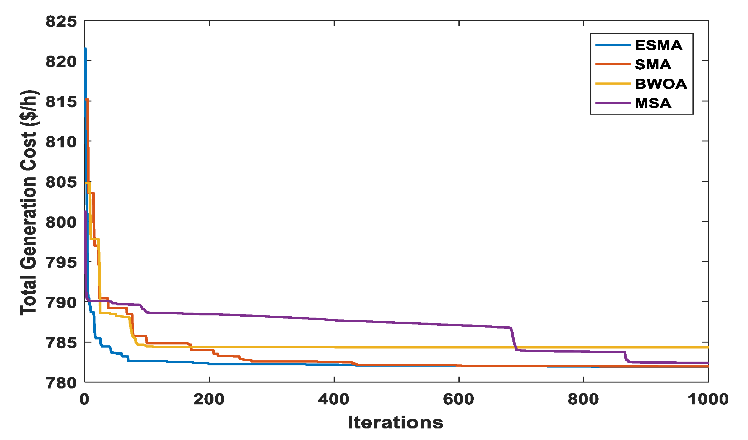
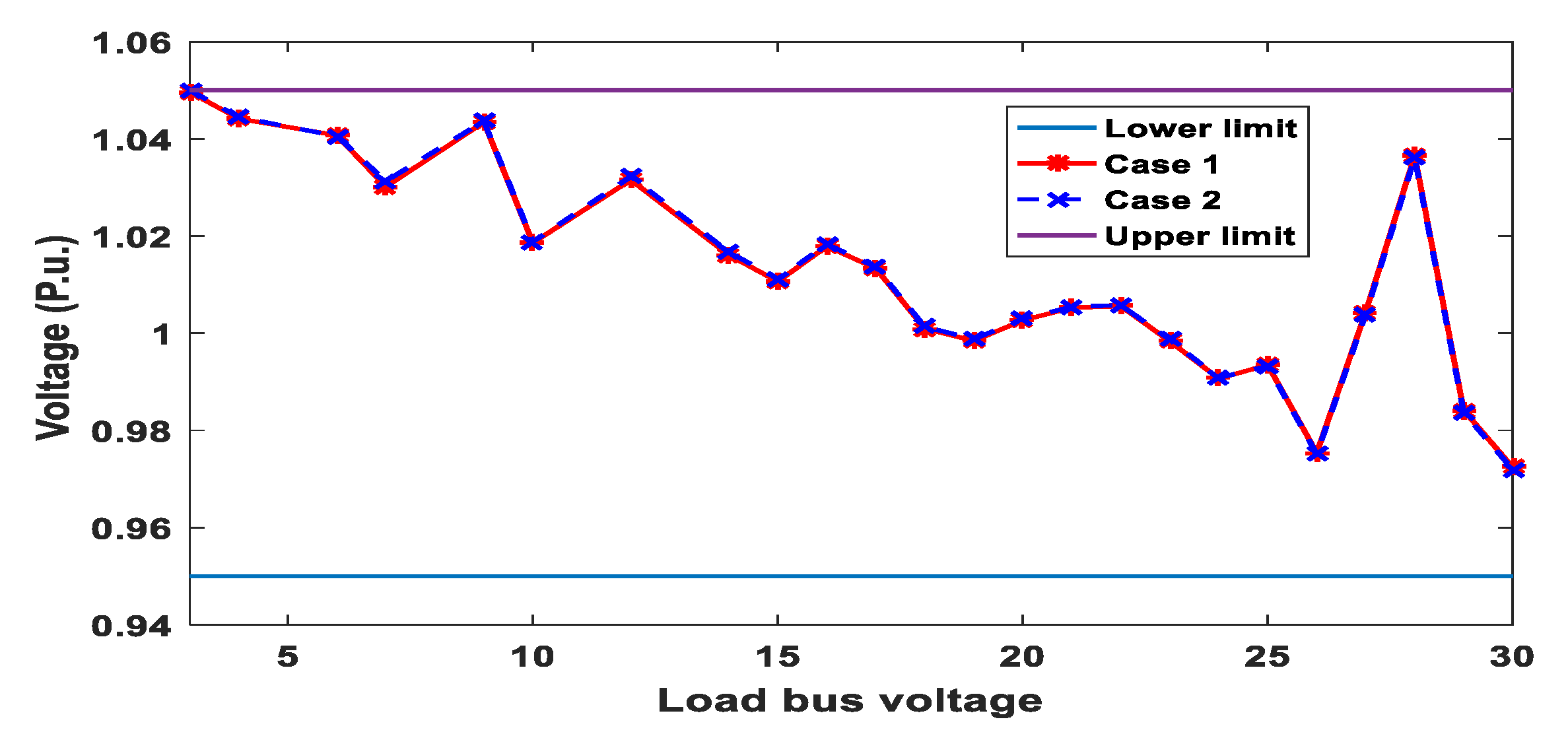
5.2.1. Case 1: Minimization of Generation Cost
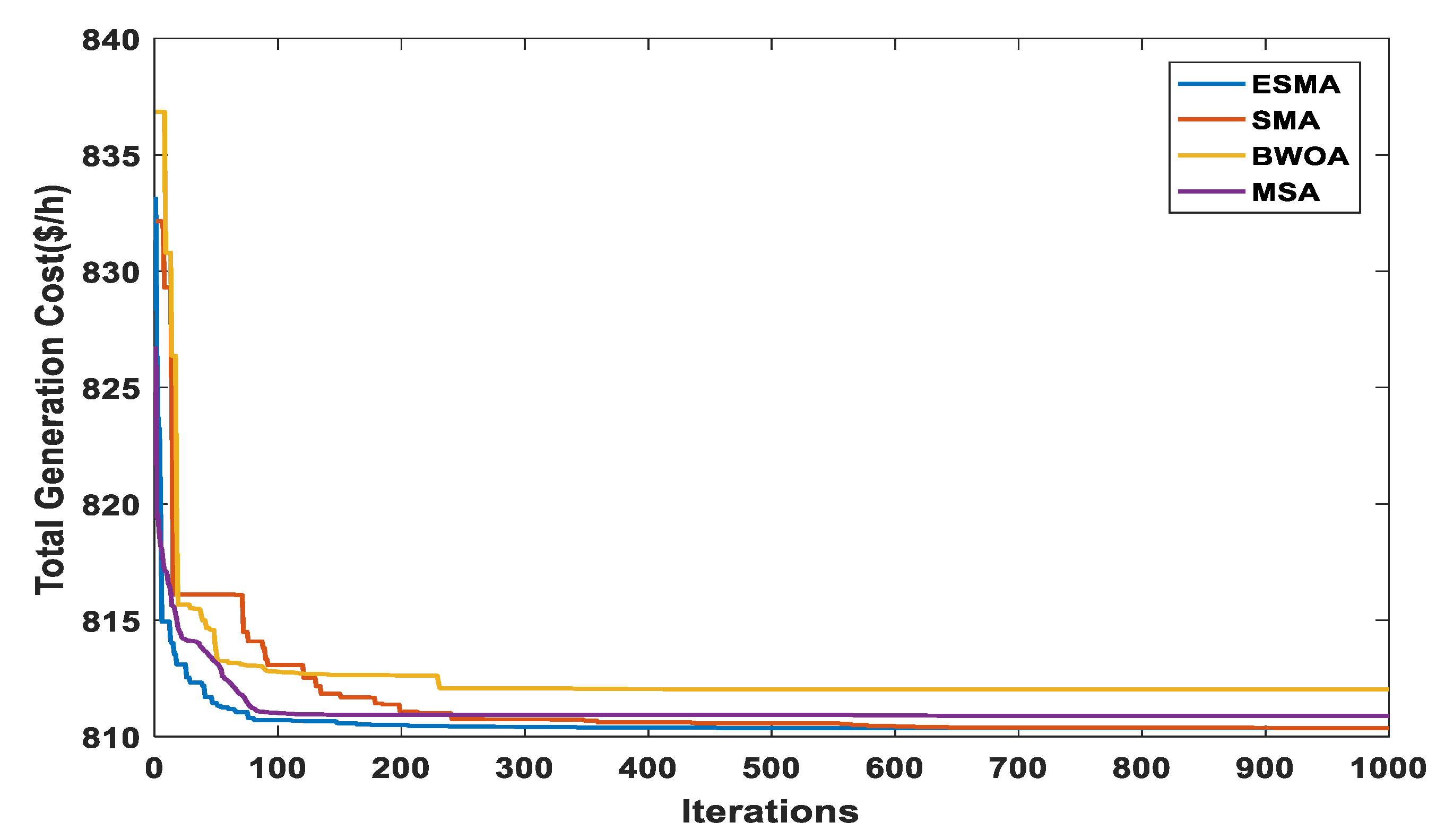
5.2.2. Case 2: Total Power Cost Minimization with Carbon Tax
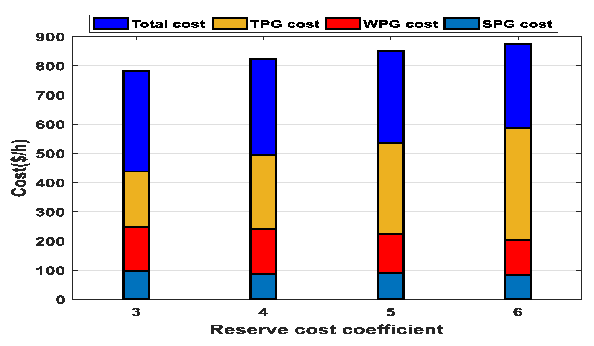
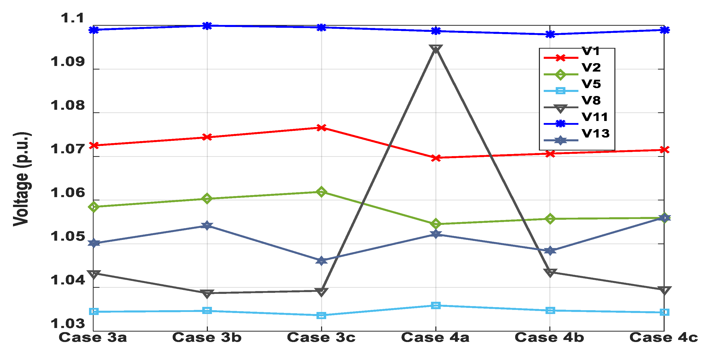
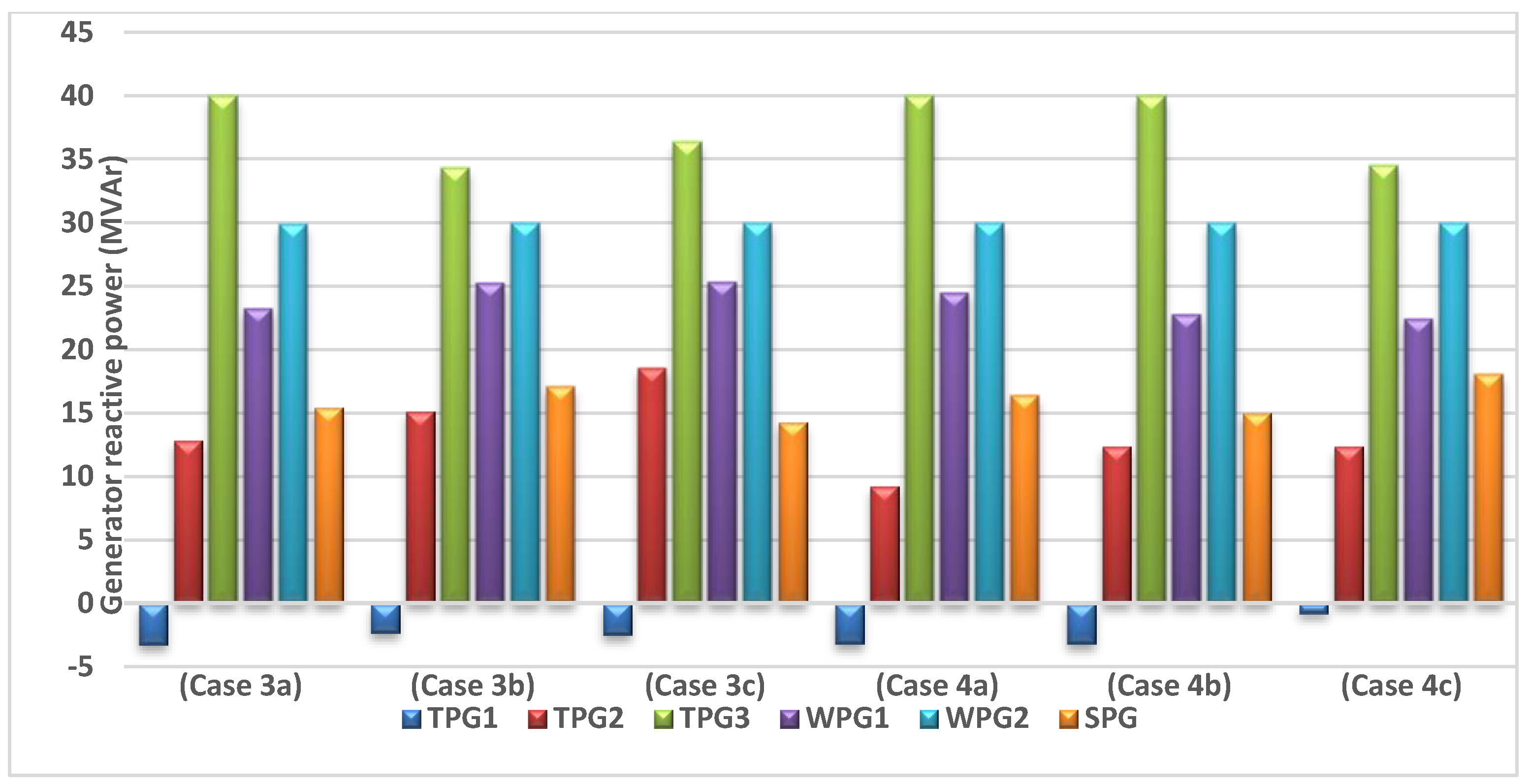
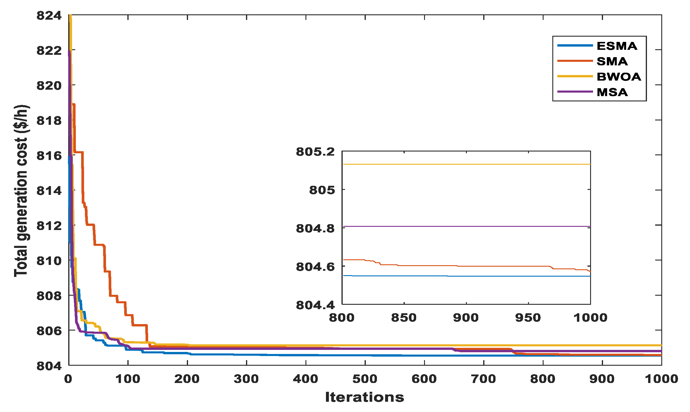
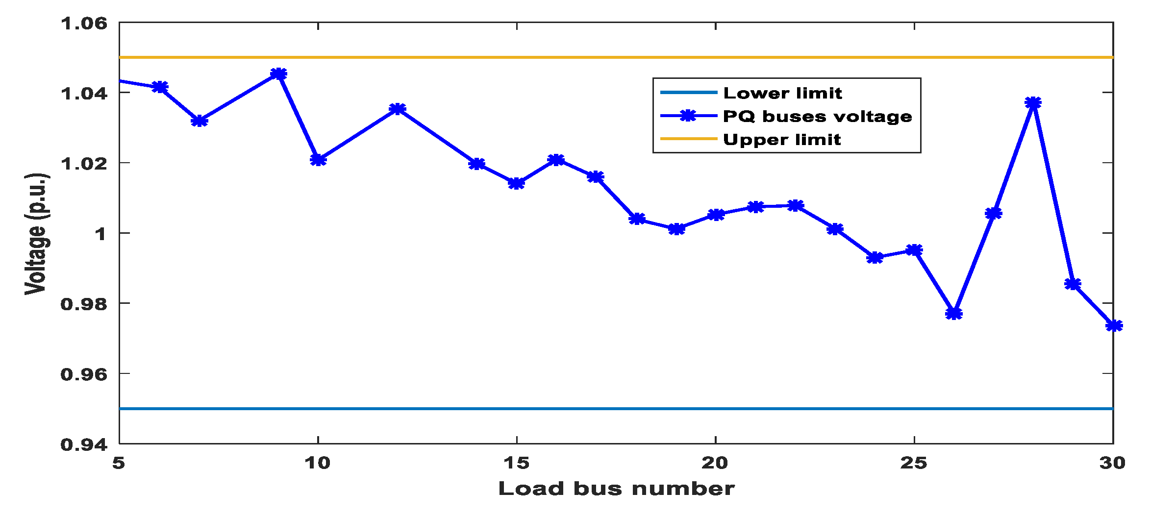
5.2.3. Case 3: Impact of Reserve Cost Variation on the Optimized Cost
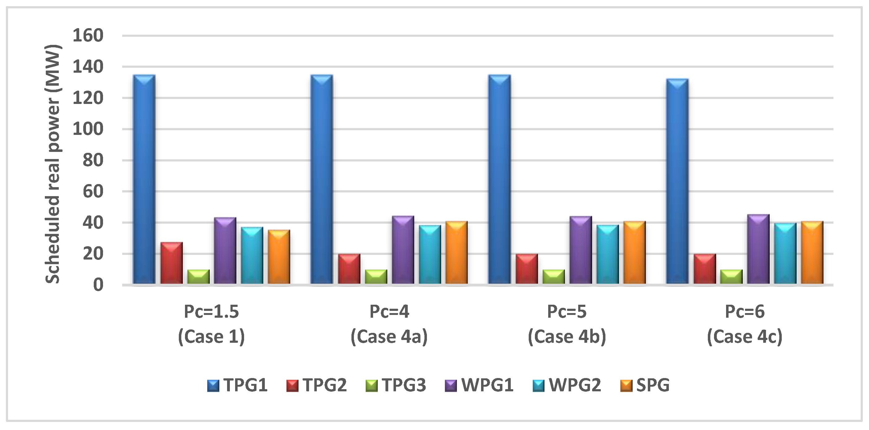
5.2.4. Case 4: Impact of Penalty Cost Variation on the Optimized Cost
5.2.5. Case 5: The Impact of Considering Ramp-Rate Limits of TPGs
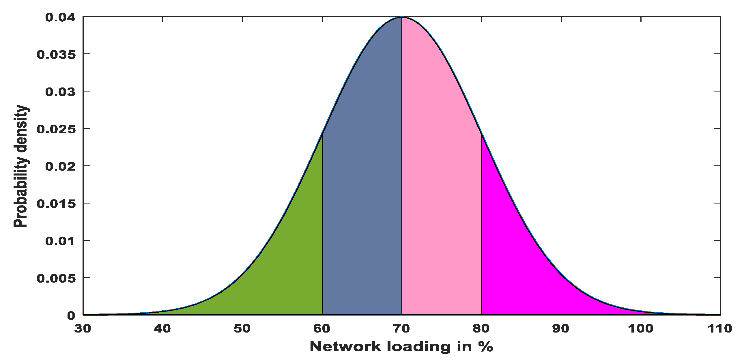
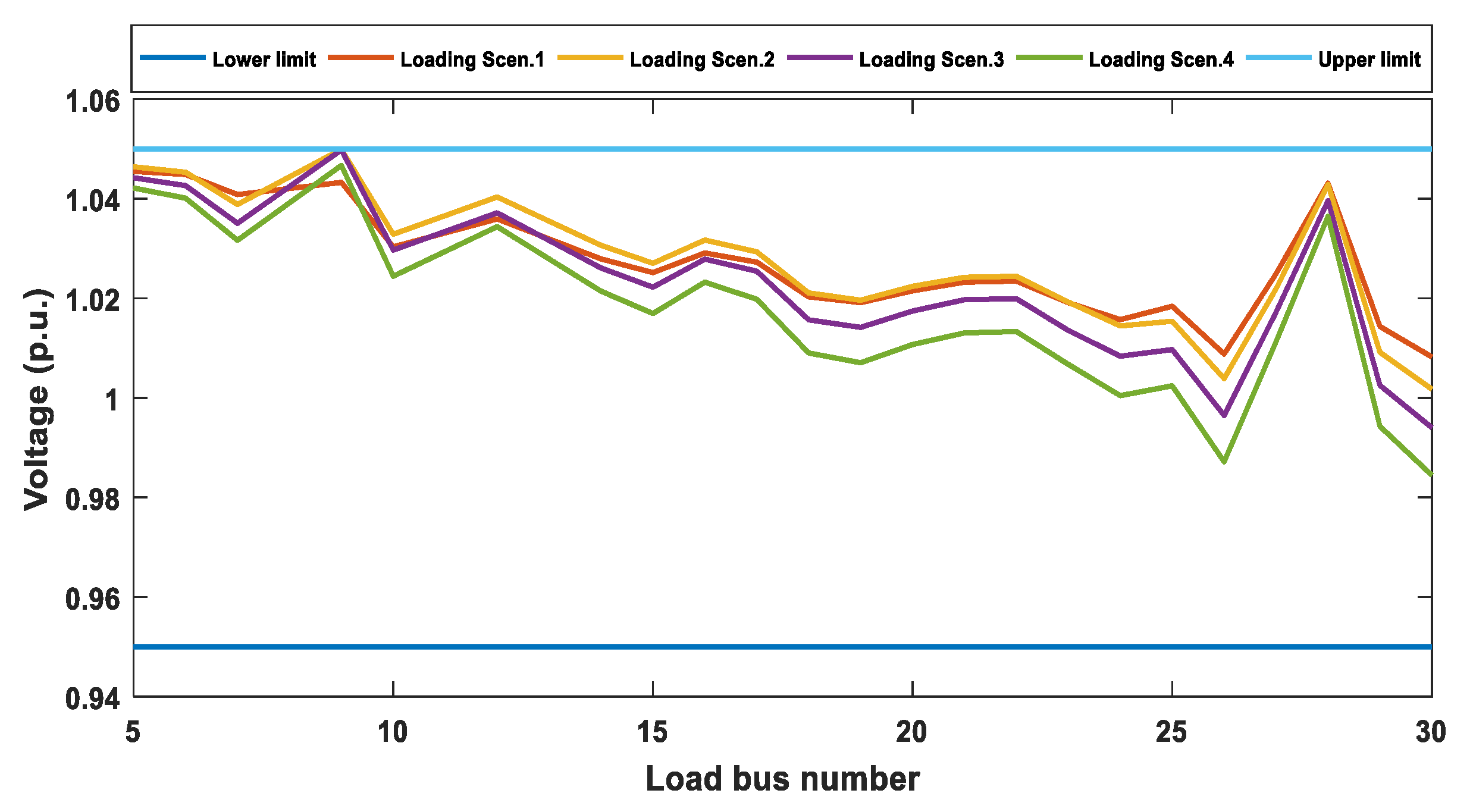
5.2.6. Case 6: The Impact of Load Demand Uncertainties
6. Conclusions
Author Contributions
Funding
Institutional Review Board Statement
Informed Consent Statement
Data Availability Statement
Acknowledgments
Conflicts of Interest
Nomenclature
| The fossil fuel cost | |
| ai, bi, and ci | Coefficients of cost for the ith TPG |
| PTPG,i | Output power from the ith TPG |
| NTPG | The number of TPGs in the power system |
| di and | Coefficients of valve-point loading |
| The minimum power of ith TPG | |
| The direct cost of wind power produced from the jth WPG | |
| Scheduled output power from the jth WPG | |
| The direct cost coefficient of the jth WPG | |
| The direct cost of the kth SPG | |
| Scheduled output power from the kth SPG | |
| The coefficient of direct cost associated with the kth SPG | |
| The reserve cost for the jth WPG | |
| The available power of the jth WPG | |
| Coefficient of reserve cost for the jth WPG | |
| Available output power from the jth WPG | |
| The Weibull PDF of the jth WPG output power | |
| Penalty cost for the jth WPG | |
| Coefficient of penalty cost for the jth WPG | |
| The rated output power of the jth WPG | |
| The reserve cost for the kth SPG | |
| Available output power from the kth SPG | |
| Coefficient of reserve cost for the kth SPG | |
| The shortage occurrence probability of solar power | |
| The expectation of being the output of SPG below the | |
| Coefficient of penalty cost of the kth SPG | |
| The surplus occurrence probability of solar power | |
| ) | The expectation of being the output of SPG above the |
| The coefficients of emissions from the ith TPG | |
| The emission cost | |
| Carbon tax | |
| Emissions (ton/h) | |
| Output power from the ith TPG at previous hour | |
| Limits of down and up ramp-rate for the ith TPG | |
| NSPG and NWPG | The number of SPGs and WPGs existing in the modified power system, respectively |
| NB | The total number of grid buses |
| The difference between voltage angles of bus i and bus j | |
| The active and reactive components of the generated power at bus i, respectively | |
| The active and reactive components of load demand at bus i, respectively | |
| The conductance and susceptance between bus i and bus j, respectively | |
| NG | The total number of generators in the system |
| NB | The total number of load buses |
| NL | The total number of system transmission lines |
| and c | Shape and scale factors of Weibull PDF, respectively |
| Vd | Voltage deviation |
| I | Solar irradiance (W/m2) |
| The cut-in, cut-out, and rated wind speeds of the wind turbine, respectively | |
| The rated power of wind turbine | |
| The solar irradiance in a standard environment (800 W/m2) | |
| Specific irradiance amount (120 W/m2) | |
| The rated power of SPG | |
| Value reduces linearly from one to zero | |
| T | The t-th iteration |
| The individual position that has the most focus on smell found currently | |
| The slime mould position | |
| and | Two individuals selected randomly from the whole population |
| S(i) | The fitness value of , i ∈ 1, 2, 3, …, n |
| R | Random value in range [0, 1] |
| bF and wF | The best and worst fitness obtained in the present iteration |
| SmellIndex | The sequence of sorting the values of fitness function |
| UB and LB | The upper and lower boundaries of the search space, respectively |
| Rand | The random value varies from 0 to 1 |
| Z | Parameter between [0, 0.1] |
| and | The high and low limits of i-th level of load demand, respectively |
References
- Carpentier, J. Contribution to the economic dispatch problem. Bull. Soc. Fr. Electr. 1962, 3, 431–447. [Google Scholar]
- Hussain, S.; Ahmed, M.A.; Kim, Y.C. Efficient Power Management Algorithm Based on Fuzzy Logic Inference for Electric Vehicles Parking Lot. IEEE Access 2019, 7, 65467–65485. [Google Scholar] [CrossRef]
- Hussain, S.; Lee, K.B.; Ahmed, M.A.; Hayes, B.; Kim, Y.C. Two-stage fuzzy logic inference algorithm for maximizing the quality of performance under the operational constraints of power grid in electric vehicle parking lots. Energies 2020, 13, 4634. [Google Scholar] [CrossRef]
- Roy, R.; Jadhav, H.T. Optimal power flow solution of power system incorporating stochastic wind power using Gbest guided artificial bee colony algorithm. Int. J. Electr. Power Energy Syst. 2015, 64, 562–578. [Google Scholar] [CrossRef]
- Panda, A.; Tripathy, M. Security constrained optimal power flow solution of wind-thermal generation system using modified bacteria foraging algorithm. Energy 2015, 93, 816–827. [Google Scholar] [CrossRef]
- Ravi, K. Optimal power flow considering intermittent wind power using particle swarm optimization. Int. J. Renew. Energy Res. 2016, 6, 504–509. [Google Scholar]
- Biswas, P.P.; Suganthan, P.N.; Amaratunga, G.A. Optimal power flow solutions incorporating stochastic wind and solar power. Energy Convers. Manag. 2017, 148, 1194–1207. [Google Scholar] [CrossRef]
- Khan, B.; Singh, P. Optimal power flow techniques under characterization of conventional and renewable energy sources: A comprehensive analysis. J. Eng. 2017, 2017, 9539506. [Google Scholar] [CrossRef] [Green Version]
- Reddy, S.S. Optimal power flow with renewable energy resources including storage. Electr. Eng. 2017, 99, 685–695. [Google Scholar] [CrossRef]
- Shaheen, M.A.; Hasanien, H.M.; Al-Durra, A. Solving of Optimal Power Flow Problem Including Renewable Energy Resources Using HEAP Optimization Algorithm. IEEE Access 2021, 9, 35846–35863. [Google Scholar] [CrossRef]
- Khazali, A.; Kalantar, M. Optimal generation dispatch incorporating wind power and responsive loads: A chance-constrained framework. J. Renew. Sustain. Energy 2015, 7, 023138. [Google Scholar] [CrossRef]
- Biswas, P.P.; Arora, P.; Mallipeddi, R.; Suganthan, P.N.; Panigrahi, B.K. Optimal placement and sizing of FACTS devices for optimal power flow in a wind power integrated electrical network. Neural Comput. Appl. 2021, 33, 6753–6774. [Google Scholar] [CrossRef]
- Chamanbaz, M.; Dabbene, F.; Lagoa, C. AC optimal power flow in the presence of renewable sources and uncertain loads. arXiv 2017, arXiv:1702.02967. [Google Scholar]
- Kaymaz, E.; Duman, S.; Guvenc, U. Optimal power flow solution with stochastic wind power using the Lévy coyote optimization algorithm. Neural Comput. Appl. 2021, 33, 6775–6804. [Google Scholar] [CrossRef]
- Khunkitti, S.; Siritaratiwat, A.; Premrudeepreechacharn, S. Multi-objective optimal power flow problems based on slime mould algorithm. Sustainability 2021, 13, 7448. [Google Scholar] [CrossRef]
- Nusair, K.; Alasali, F.; Hayajneh, A.; Holderbaum, W. Optimal placement of FACTS devices and power-flow solutions for a power network system integrated with stochastic renewable energy resources using new metaheuristic optimization techniques. Int. J. Energy Res. 2021, 45, 18786–18809. [Google Scholar] [CrossRef]
- ElSayed, S.K.; Elattar, E.E. Slime Mold Algorithm for Optimal Reactive Power Dispatch Combining with Renewable Energy Sources. Sustainability 2021, 13, 5831. [Google Scholar] [CrossRef]
- Wei, Y.; Zhou, Y.; Luo, Q.; Deng, W. Optimal reactive power dispatch using an improved slime mould algorithm. Energy Rep. 2021, 7, 8742–8759. [Google Scholar] [CrossRef]
- Li, S.; Chen, H.; Wang, M.; Heidari, A.A.; Mirjalili, S. Slime mould algorithm: A new method for stochastic optimization. Future Gener. Comput. Syst. 2020, 111, 300–323. [Google Scholar] [CrossRef]
- Tu, J.; Chen, H.; Wang, M.; Gandomi, A.H. The Colony Predation Algorithm. J. Bionic Eng. 2021, 18, 674–710. [Google Scholar] [CrossRef]
- Abualigah, L.; Yousri, D.; Abd Elaziz, M.; Ewees, A.A.; Al-qaness, M.A.; Gandomi, A.H. Aquila Optimizer: A novel meta-heuristic optimization Algorithm. Comput. Ind. Eng. 2021, 157, 107250. [Google Scholar] [CrossRef]
- Ahmadianfar, I.; Heidari, A.A.; Gandomi, A.H.; Chu, X.; Chen, H. RUN beyond the metaphor: An efficient optimization algorithm based on Runge Kutta method. Expert Syst. Appl. 2021, 181, 115079. [Google Scholar] [CrossRef]
- Peña-Delgado, A.F.; Peraza-Vázquez, H.; Almazán-Covarrubias, J.H.; Torres-Cruz, N.; García-Vite, P.M.; Morales-Cepeda, A.B.; Ramirez-Arredondo, J.M. A Novel Bio-Inspired Algorithm Applied to Selective Harmonic Elimination in a Three-Phase Eleven-Level Inverter. Math. Probl. Eng. 2020, 2020, 8856040. [Google Scholar] [CrossRef]
- Mohamed, A. Moth Swarm Algorithm (MSA). MATLAB Central File Exchange. 10 September 2021. Available online: https://www.mathworks.com/matlabcentral/fileexchange/57822-moth-swarm-algorithm-msa (accessed on 15 November 2021).
- Chaib, A.E.; Bouchekara, H.R.; Mehasni, R.; Abido, M.A. Optimal power flow with emission and non-smooth cost functions using backtracking search optimization algorithm. Int. J. Electr. Power Energy Syst. 2016, 81, 64–77. [Google Scholar] [CrossRef]
- Chang, T.P. Investigation on frequency distribution of global radiation using different probability density functions. Int. J. Appl. Sci. Eng. 2010, 8, 99–107. [Google Scholar]
- Shi, L.; Wang, C.; Yao, L.; Ni, Y.; Bazargan, M. Optimal power flow solution incorporating wind power. IEEE Syst. J. 2011, 6, 233–241. [Google Scholar] [CrossRef]
- Yao, F.; Dong, Z.Y.; Meng, K.; Xu, Z.; Iu, H.H.; Wong, K.P. Quantum-inspired particle swarm optimization for power system operations considering wind power uncertainty and carbon tax in Australia. IEEE Trans. Ind. Inform. 2012, 8, 880–888. [Google Scholar] [CrossRef]
- Alsac, O.; Stott, B. Optimal load flow with steady-state security. IEEE Trans. Power Appar. Syst. 1974, PAS-93, 745–751. [Google Scholar] [CrossRef] [Green Version]
- IEC I. 61400e1: Wind Turbines Part 1: Design Requirements; International Electrotechnical Commission: Geneva, Switzerland, 2005.
- Reddy, S.S.; Bijwe, P.R.; Abhyankar, A.R. Real-time economic dispatch considering renewable power generation variability and uncertainty over scheduling period. IEEE Syst. J. 2014, 9, 1440–1451. [Google Scholar] [CrossRef]
- Dubey, H.M.; Pandit, M.; Panigrahi, B.K. Hybrid flower pollination algorithm with time-varying fuzzy selection mechanism for wind integrated multi-objective dynamic economic dispatch. Renew. Energy 2015, 83, 188–202. [Google Scholar] [CrossRef]
- Lai, L.L.; Ma, J.T.; Yokoyama, R.; Zhao, M. Improved genetic algorithms for optimal power flow under both normal and contingent operation states. Int. J. Electr. Power Energy Syst. 1997, 19, 287–292. [Google Scholar] [CrossRef]
- Howard, F.L. The life history of Physarum polycephalum. Am. J. Bot. 1931, 18, 116–133. [Google Scholar] [CrossRef]
- Nadimi-Shahraki, M.H.; Taghian, S.; Mirjalili, S. An improved grey wolf optimizer for solving engineering problems. Expert Syst. Appl. 2021, 166, 113917. [Google Scholar] [CrossRef]
- Niknam, T.; Narimani, M.R.; Aghaei, J.; Tabatabaei, S.; Nayeripour, M. Modified honey bee mating optimisation to solve dynamic optimal power flow considering generator constraints. IET Gener. Transm. Distrib. 2011, 5, 989–1002. [Google Scholar] [CrossRef]
- Mohseni-Bonab, S.M.; Rabiee, A.; Mohammadi-Ivatloo, B. Voltage stability constrained multi-objective optimal reactive power dispatch under load and wind power uncertainties: A stochastic approach. Renew. Energy 2016, 85, 598–609. [Google Scholar] [CrossRef]


| Gen. | Bus | a | B | c | d | e | α | β | ω | μ | ||||
|---|---|---|---|---|---|---|---|---|---|---|---|---|---|---|
| TPG1 | 1 | 0 | 2 | 0.00375 | 18 | 0.037 | 4.091 | −5.554 | 6.49 | 0.0002 | 6.667 | 99.211 | 20 | 15 |
| TPG2 | 2 | 0 | 1.75 | 0.0175 | 16 | 0.038 | 2.543 | −6.047 | 5.638 | 0.0005 | 3.333 | 80 | 15 | 10 |
| TPG3 | 8 | 0 | 3.25 | 0.00834 | 12 | 0.045 | 5.326 | −3.55 | 3.38 | 0.002 | 2 | 20 | 8 | 4 |
| Item | Number | Details |
|---|---|---|
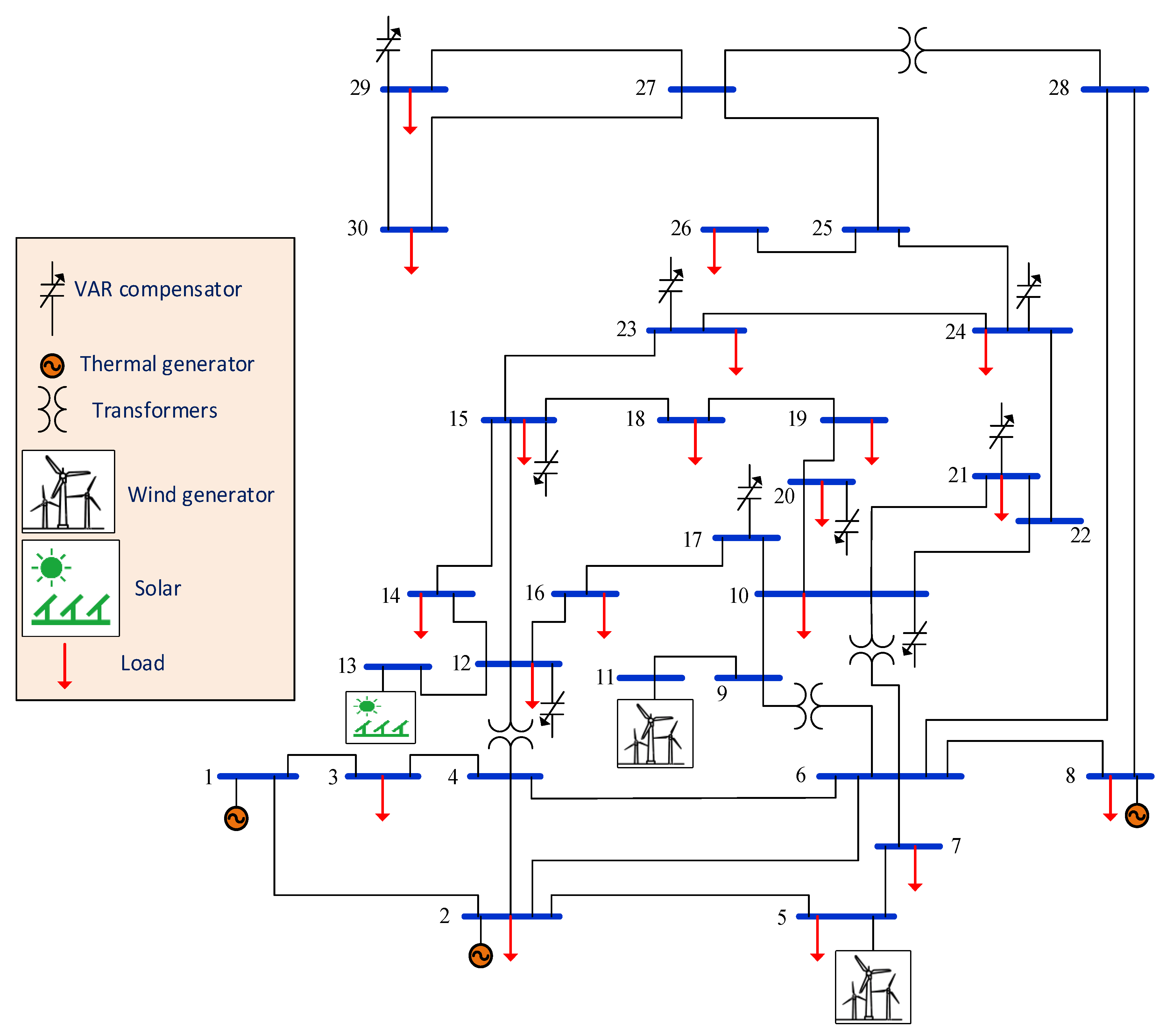
| Buses | 30 | [29] |
| Branches | 41 | [29] |
| TPGs (TPG1, TPG2, and TPG3) | 3 | Connected at bus 1 (swing), bus 2, and bus 8 |
| WPGs (WPG1 and WPG2) | 2 | Connected at bus 5 and bus 11 |
| SPG | 1 | Connected at bus 13 |
| Control variables | 11 | The scheduled output power of: TPG2, TPG3, WPG1, WPG2, SPG, and generator buses voltages (6 generators) |
| Connected load | - | 283.4 MW, 126.2 MVAR |
| Allowable voltage range for load buses | 24 | [0.95–1.05] p.u. |
| WPGs | SPG | ||||||
|---|---|---|---|---|---|---|---|
| WPG | No. of Turbines | Rated Power (Pwr) | Weibull PDF Parameters | Weibull Mean, Mwbl | Rated Power, Psr | Lognormal PDF Parameters | Lognormal Mean, Mlogn |
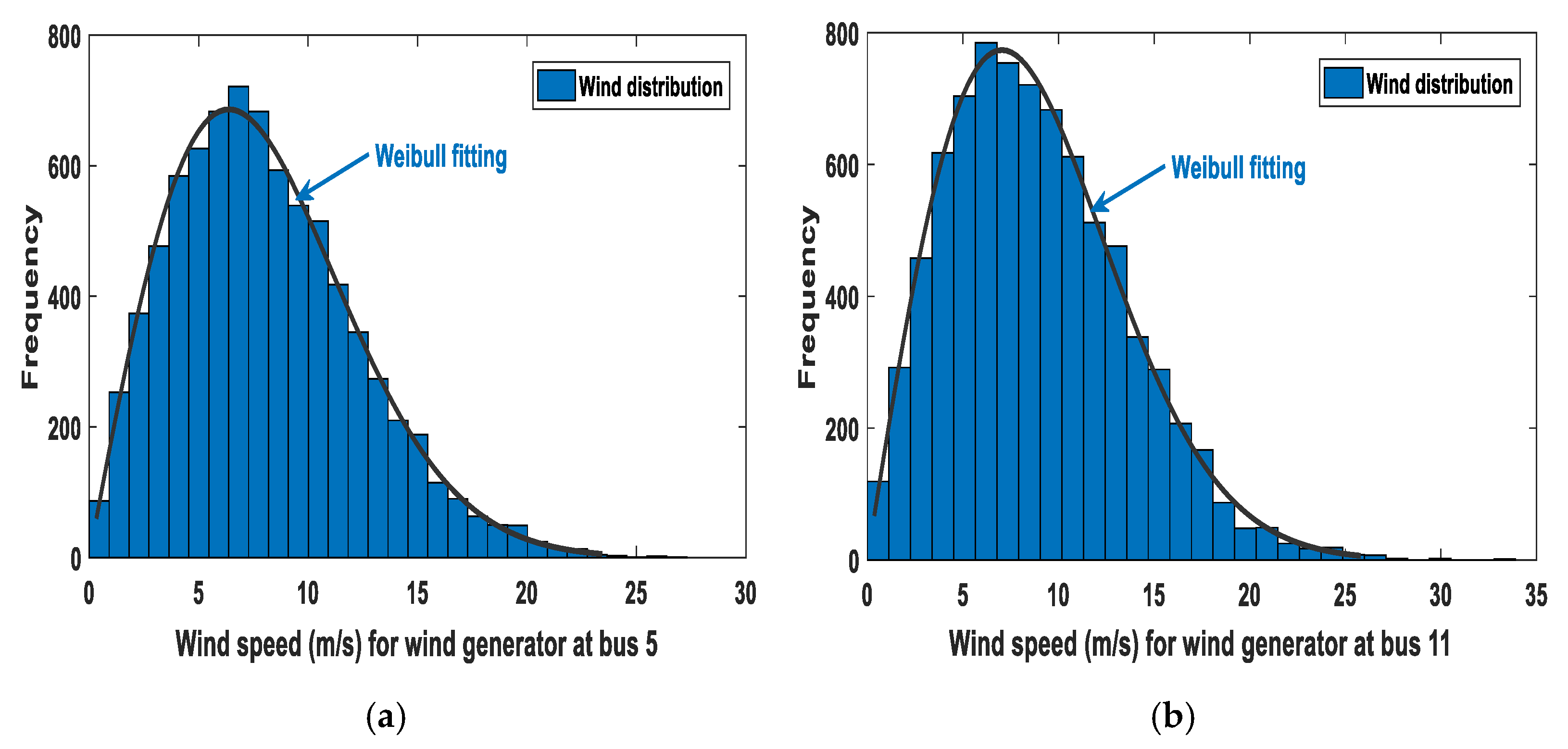
| 1 (at bus 5) | 25 | 75 MW | k = 2, c = 9 | v = 7.976 (m/s) | |||
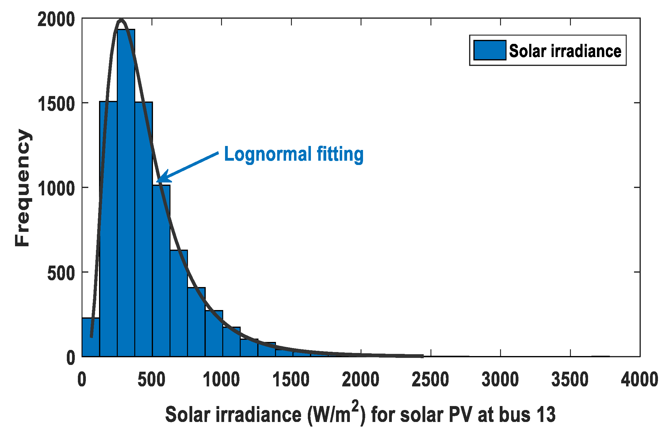
| 2 (at bus 11) | 20 | 60 MW | k = 2, c = 10 | v = 8.862 (m/s) | 50 MW (at bus 13) | δ = 0.6, μ = 6 | I = 483 (W/m2) |
| Function | ESMA | SMA | CPA | AO | RUN | |
|---|---|---|---|---|---|---|
| F1 | Best | 0.00 | 1.8 × 10−293 | 6.5 × 10−190 | 7.15 × 10−76 | 9.07 × 10−86 |
| Worst | 5.4 × 10−295 | 1.1 × 10−156 | 1.41 × 10−70 | 4.17 × 10−57 | 1 × 10−75 | |
| Mean | 2.7 × 10−296 | 5.3 × 10−158 | 7.07 × 10−72 | 2.09 × 10−58 | 5.02 × 10−77 | |
| Std | 0.00 | 2.4 × 10−157 | 3.16 × 10−71 | 9.33 × 10−58 | 2.24 × 10−76 | |
| F2 | Best | 7.4 × 10−162 | 2.9 × 10−132 | 4.8 × 10−106 | 1.3 × 10−36 | 1.04 × 10−47 |
| Worst | 1.9 × 10−148 | 1.02 × 10−64 | 1.07 × 10⁻¹⁴ | 9.5 × 10⁻³² | 2.3 × 10−42 | |
| Mean | 1.8 × 10−149 | 5.1 × 10−66 | 5.36 × 10⁻¹⁶ | 1.37 × 10⁻³² | 1.87 × 10−43 | |
| Std | 5.1 × 10−149 | 2.28 × 10−65 | 2.4 × 10⁻¹⁵ | 3.28 × 10⁻³² | 5.35 × 10−43 | |
| F3 | Best | 0.00 | 1.1 × 10−254 | 2.2 × 10−186 | 3.39 × 10−71 | 5.75 × 10−77 |
| Worst | 2.1 × 10−298 | 1.4 × 10−140 | 2.51 × 10⁻²⁶ | 1.58 × 10−62 | 4.54 × 10−61 | |
| Mean | 1.8 × 10−299 | 6.8 × 10−142 | 1.26 × 10⁻²⁷ | 1.28 × 10−63 | 2.33 × 10−62 | |
| Std | 0.00 | 3 × 10−141 | 5.61 × 10⁻²⁷ | 3.7 × 10−63 | 1.01 × 10−61 | |
| F4 | Best | 8.9 × 10−159 | 5.7 × 10−137 | 3.78 × 10−97 | 8.91 × 10−40 | 1.35 × 10−42 |
| Worst | 3.8 × 10−146 | 9.02 × 10−51 | 3.54 × 10⁻¹⁹ | 1.67 × 10⁻³¹ | 4.16 × 10⁻³⁴ | |
| Mean | 1.9 × 10−147 | 4.51 × 10−52 | 1.77 × 10⁻²⁰ | 1.26 × 10⁻³² | 2.09 × 10⁻³⁵ | |
| Std | 8.5 × 10−147 | 2.02 × 10−51 | 7.93 × 10⁻²⁰ | 4.05 × 10⁻³² | 9.3 × 10⁻³⁵ | |
| F5 | Best | 26.08305 | 25.34758 | 28.12882 | 24.13219 | 23.34961 |
| Worst | 28.94341 | 28.98832 | 28.88188 | 29.26575 | 26.52757 | |
| Mean | 28.24751 | 28.57338 | 28.53022 | 26.85075 | 24.73586 | |
| Std | 0.854929 | 0.807162 | 0.196671 | 1.924605 | 0.832917 | |
| F6 | Best | 0.205897 | 0.01122 | 0.000936 | 1.61 × 10⁻⁸ | 7.23 × 10⁻⁹ |
| Worst | 4.076296 | 3.74817 | 1.069296 | 0.000556 | 2.24 × 10⁻⁸ | |
| Mean | 1.054545 | 0.810915 | 0.293309 | 0.000145 | 1.19 × 10⁻⁸ | |
| Std | 0.980102 | 0.967813 | 0.368271 | 0.000182 | 3.7 × 10⁻⁹ | |
| F7 | Best | 3.22 × 10⁻⁵ | 1.84 × 10⁻⁵ | 3.23 × 10⁻⁵ | 6.04 × 10⁻⁶ | 3.74 × 10⁻⁵ |
| Worst | 0.003883 | 0.00744 | 0.009786 | 0.000818 | 0.000865 | |
| Mean | 0.001199 | 0.001253 | 0.00206 | 0.00021 | 0.00042 | |
| Std | 0.001113 | 0.00176 | 0.002655 | 0.000197 | 0.000268 |
| Function | ESMA | SMA | CPA | AO | RUN | |
|---|---|---|---|---|---|---|
| F8 | Best | −1850.29 | −1909.03 | −1909.03 | −1901.64 | −1660.17 |
| Worst | −1460.88 | −941.222 | −841.176 | −718.461 | −1397.78 | |
| Mean | −1653.2 | −1854.84 | −1665.13 | −1061.31 | −1580.75 | |
| Std | 102.5683 | 215.5892 | 266.4826 | 353.9877 | 78.84949 | |
| F9 | Best | 0.00 | 0.00 | 0.00 | 0.00 | 0.00 |
| Worst | 0.00 | 0.00 | 0.00 | 0.00 | 0.00 | |
| Mean | 0.00 | 0.00 | 0.00 | 0.00 | 0.00 | |
| Std | 0.00 | 0.00 | 0.00 | 0.00 | 0.00 | |
| F10 | Best | 8.88 × 10⁻¹⁶ | 8.88 × 10⁻¹⁶ | 8.88 × 10⁻¹⁶ | 8.88 × 10⁻¹⁶ | 8.88 × 10⁻¹⁶ |
| Worst | 8.88 × 10⁻¹⁶ | 8.88 × 10⁻¹⁶ | 1.87 × 10⁻¹⁴ | 8.88 × 10⁻¹⁶ | 8.88 × 10⁻¹⁶ | |
| Mean | 8.88 × 10⁻¹⁶ | 8.88 × 10⁻¹⁶ | 1.78 × 10⁻¹⁵ | 8.88 × 10⁻¹⁶ | 8.88 × 10⁻¹⁶ | |
| Std | 0.00 | 0.00 | 0.00 | 3.97 × 10⁻¹⁵ | 0.00 | |
| F11 | Best | 0.00 | 0.00 | 0.00 | 0.00 | 0.00 |
| Worst | 0.00 | 0.00 | 0.00 | 0.00 | 0.00 | |
| Mean | 0.00 | 0.00 | 0.00 | 0.00 | 0.00 | |
| Std | 0.00 | 0.00 | 0.00 | 0.00 | 0.00 | |
| F12 | Best | 0.019339 | 0.000221 | 3.04 × 10⁻⁵ | 1.05 × 10⁻¹⁰ | 2.99 × 10⁻⁹ |
| Worst | 0.224734 | 0.883664 | 0.073697 | 5.46 × 10⁻⁶ | 1.57 × 10⁻⁸ | |
| Mean | 0.055819 | 0.053203 | 0.012284 | 6.23 × 10⁻⁷ | 6.93 × 10⁻⁹ | |
| Std | 0.046062 | 0.195804 | 0.01766 | 1.2 × 10⁻⁶ | 3.43 × 10⁻⁹ | |
| F13 | Best | 0.997042 | 0.007141 | 0.003875 | 1.82 × 10⁻⁷ | 4.07 × 10⁻⁸ |
| Worst | −1850.29 | −1909.03 | −1909.03 | −1901.64 | −1660.17 | |
| Mean | −1460.88 | −941.222 | −841.176 | −718.461 | −1397.78 | |
| Std | −1653.2 | −1854.84 | −1665.13 | −1061.31 | −1580.75 |
| Function | ESMA | SMA | CPA | AO | RUN | |
|---|---|---|---|---|---|---|
| F14 | Best | 0.998004 | 0.998004 | 0.998004 | 0.998004 | 0.998004 |
| Worst | 7.873993 | 12.67051 | 12.67051 | 12.67051 | 10.76318 | |
| Mean | 2.528537 | 2.517909 | 2.953424 | 2.573682 | 2.081493 | |
| Std | 2.107136 | 3.145931 | 3.84665 | 2.574285 | 2.241941 | |
| F15 | Best | 0.00 | 1.1 × 10−254 | 2.2 × 10−186 | 0.000325 | 0.000307 |
| Worst | 2.1 × 10−298 | 1.4 × 10−140 | 2.51 × 10⁻²⁶ | 0.001155 | 0.001223 | |
| Mean | 1.8 × 10−299 | 6.8 × 10−142 | 1.26 × 10⁻²⁷ | 0.00053 | 0.00072 | |
| Std | 0.00 | 3 × 10−141 | 5.61 × 10⁻²⁷ | 0.00018 | 0.000467 | |
| F16 | Best | −1.03163 | −1.03163 | −1.03163 | −1.03163 | −1.03163 |
| Worst | −1.03161 | −1.03013 | −1.03163 | −1.02995 | −1.03163 | |
| Mean | −1.03163 | −1.03155 | −1.03163 | −1.03104 | −1.03163 | |
| Std | 4.12 × 10⁻⁶ | 0.000335 | 9.56 × 10⁻¹⁰ | 0.000547 | 8.13 × 10⁻¹² | |
| F17 | Best | 0.397887 | 0.397887 | 0.397887 | 0.397893 | 0.397887 |
| Worst | 0.397887 | 0.397894 | 0.399219 | 0.399082 | 0.397887 | |
| Mean | 0.397887 | 0.397889 | 0.397954 | 0.398149 | 0.397887 | |
| Std | 2.12 × 10⁻¹⁰ | 1.94 × 10⁻⁶ | 0.000298 | 0.000274 | 4.27 × 10⁻¹² | |
| F18 | Best | 3 | 3 | 3 | 3.00648 | 3 |
| Worst | 3 | 30.00163 | 30 | 3.100674 | 3 | |
| Mean | 3 | 7.050142 | 4.663726 | 3.042457 | 3 | |
| Std | 2.37 × 10⁻¹⁴ | 9.89173 | 6.125915 | 0.02737 | 5.41 × 10⁻¹³ | |
| F19 | Best | −0.30048 | −0.30048 | −0.30048 | −0.30048 | −0.30048 |
| Worst | −0.30048 | −0.30048 | −0.30038 | −0.30048 | −0.30048 | |
| Mean | −0.30048 | −0.30048 | −0.30047 | −0.30048 | −0.30048 | |
| Std | 1.14 × 10⁻¹⁶ | 1.14 × 10⁻¹⁶ | 2.19 × 10⁻⁵ | 1.14 × 10⁻¹⁶ | 1.14 × 10⁻¹⁶ | |
| F20 | Best | −3.322 | −3.32198 | −3.322 | −3.2947 | −3.322 |
| Worst | −3.2031 | −0.19258 | −3.14355 | −2.67041 | −3.20309 | |
| Mean | −3.28612 | −3.06081 | −3.29758 | −3.1067 | −3.28038 | |
| Std | 0.055765 | 0.747204 | 0.050586 | 0.143442 | 0.058183 | |
| F21 | Best | −10.1532 | −10.1531 | −5.0552 | −10.1527 | −10.1532 |
| Worst | −5.05074 | −5.05489 | −4.20446 | −10.1019 | −5.0552 | |
| Mean | −5.81968 | −8.87754 | −5.00614 | −10.1365 | −8.3689 | |
| Std | 1.867737 | 2.25068 | 0.190098 | 0.016429 | 2.494761 | |
| F22 | Best | −10.4029 | −10.4029 | −5.08767 | −10.4028 | −10.4029 |
| Worst | −5.0865 | −5.12737 | −4.97896 | −10.3216 | −5.08767 | |
| Mean | −6.94796 | −9.8648 | −5.08015 | −10.3889 | −9.07412 | |
| Std | 2.601126 | 1.620212 | 0.025303 | 0.019955 | 2.36137 | |
| F23 | Best | −10.5364 | −10.5363 | −10.5364 | −10.5362 | −10.5364 |
| Worst | −4.63728 | −5.12744 | −4.82737 | −10.4701 | −5.12848 | |
| Mean | −6.7263 | −9.99261 | −5.6062 | −10.5212 | −9.18443 | |
| Std | 2.561402 | 1.655735 | 1.540624 | 0.019921 | 2.402536 |
| Control Variables | Min. | Max. | ESMA | SMA | BWOA | MSA |
|---|---|---|---|---|---|---|
| PTG1 (MW) | 50 | 140 | 134.9143078 | 134.9126665 | 134.9318602 | 134.9080709 |
| PTG2 (MW) | 20 | 80 | 27.68805837 | 28.41701 | 30.52148 | 29.91749 |
| PTG3 (MW) | 10 | 35 | 10.01257102 | 10 | 10.02768 | 41.42875 |
| Pws,1 (MW) | 0 | 75 | 43.57823017 | 43.97604 | 43.11587 | 10.15632 |
| Pws,2 (MW) | 0 | 60 | 37.45089 | 36.74404 | 37.82475 | 37.68851 |
| Pss (MW) | 0 | 50 | 35.5275 | 35.11807 | 33.36969 | 35.20921 |
| V1 (p.u.) | 0.95 | 1.1 | 1.069956 | 1.072577 | 1.069029 | 1.071379 |
| V2 (p.u.) | 0.95 | 1.1 | 1.056832 | 1.057642 | 1.099901 | 1.057197 |
| V5 (p.u.) | 0.95 | 1.1 | 1.033471 | 1.037017 | 1.095503 | 1.079234 |
| V8 (p.u.) | 0.95 | 1.1 | 1.088021 | 1.040221 | 1.02164 | 1.075681 |
| V11 (p.u.) | 0.95 | 1.1 | 1.097041 | 1.097474 | 1.00625 | 1.07746 |
| V13 (p.u.) | 0.95 | 1.1 | 1.052377 | 1.048536 | 1.067481 | 1.047355 |
| QTG1 (MVAr) | −20 | 150 | −6.58886 | −1.73162 | −20 | −3.94493 |
| QTG2 (MVAr) | −20 | 60 | 16.43639 | 12.89954 | 60 | 7.538948 |
| QTG3 (MVAr) | −15 | 40 | 40 | 35.9758 | 15.65167 | 40 |
| Qws,1 (MVAr) | −30 | 35 | 21.18113 | 24.64654 | 35 | 35 |
| Qws,2 (MVAr) | −25 | 30 | 29.5482 | 30 | 2.883899 | 22.88516 |
| Qss (MVAr) | −20 | 25 | 16.47241 | 15.1557 | 25 | 15.4901 |
| Total power cost ($/h) | 781.9375819 | 781.9580658 | 784.3423563 | 782.4230422 | ||
| Emissions (t/h) | 1.762973771 | 1.76261913 | 1.764219911 | 1.76173491 | ||
| Carbon tax, Ctax ($/h) | 0 | 0 | 0 | 0 | ||
| Ploss (MW) | 5.771556781 | 5.76783193 | 6.401297765 | 5.908352008 | ||
| Vd (p.u.) | 0.458684989 | 0.451488019 | 0.53484521 | 0.443429768 |
| Control Variables | Min. | Max. | ESMA | SMA | BWOA | MSA |
|---|---|---|---|---|---|---|
| PTG1 (MW) | 50 | 140 | 123.4182597 | 123.558571 | 123.9385776 | 123.0458701 |
| PTG2 (MW) | 20 | 80 | 32.8988 | 32.70381 | 31.55832 | 31.94699 |
| PTG3 (MW) | 10 | 35 | 10.00018 | 10 | 10.02575 | 10.00019 |
| Pws,1 (MW) | 0 | 75 | 45.87829 | 46.01788 | 43.52164 | 45.40579 |
| Pws,2 (MW) | 0 | 60 | 38.84621 | 38.76592 | 38.18338 | 38.19805 |
| Pss (MW) | 0 | 50 | 37.63186 | 37.63258 | 41.63565 | 40.09511 |
| V1 (p.u.) | 0.95 | 1.1 | 1.070554 | 1.069455 | 1.076582 | 1.067868 |
| V2 (p.u.) | 0.95 | 1.1 | 1.057246 | 1.056339 | 1.060155 | 1.055309 |
| V5 (p.u.) | 0.95 | 1.1 | 1.036466 | 1.034248 | 1.033567 | 1.031957 |
| V8 (p.u.) | 0.95 | 1.1 | 1.040751 | 1.082863 | 1.031061 | 1.040321 |
| V11 (p.u.) | 0.95 | 1.1 | 1.099149 | 1.1 | 1.07291 | 1.099459 |
| V13 (p.u.) | 0.95 | 1.1 | 1.053391 | 1.053591 | 1.056897 | 1.1 |
| QTG1 (MVAr) | −20 | 150 | −3.04826 | −4.14907 | 6.942384 | −6.10507 |
| QTG2 (MVAr) | −20 | 60 | 12.62003 | 12.03468 | 18.60405 | 12.98216 |
| QTG3 (MVAr) | −15 | 40 | 35.90165 | 40 | 24.44273 | 34.59923 |
| Qws,1 (MVAr) | −30 | 35 | 23.35533 | 21.07284 | 22.66046 | 19.91761 |
| Qws,2 (MVAr) | −25 | 30 | 30 | 30 | 22.74522 | 29.40543 |
| Qss (MVAr) | −20 | 25 | 16.83568 | 16.72546 | 20.55141 | 25 |
| Total power cost ($/h) | 810.3557515 | 810.3738858 | 812.0366457 | 810.8842547 | ||
| Emissions (t/h) | 0.88593426 | 0.893157637 | 0.913174063 | 0.867357442 | ||
| Carbon tax, Ctax ($/h) | 20 | 20 | 20 | 20 | ||
| Ploss (MW) | 5.273603276 | 5.278762466 | 5.463313439 | 5.291996546 | ||
| Vd (p.u.) | 0.464133712 | 0.467254932 | 0.450579985 | 0.538738367 |
| Control Variables | Min. | Max. | ESMA | SMA | BWOA | MSA |
|---|---|---|---|---|---|---|
| PTG1 (MW) | 79.211 | 114.211 | 92.16880318 | 92.44231076 | 90.18995958 | 91.32417994 |
| PTG2 (MW) | 65 | 80 | 65.00002 | 65 | 65 | 65 |
| PTG3 (MW) | 12 | 24 | 12 | 12 | 12.26708 | 12 |
| Pws,1 (MW) | 0 | 75 | 44.16894 | 43.88145 | 43.08437 | 44.17037 |
| Pws,2 (MW) | 0 | 60 | 37.37163 | 37.4186 | 37.35422 | 37.33551 |
| Pss (MW) | 0 | 50 | 37.31031 | 37.29943 | 40.20372 | 38.24819 |
| V1 (p.u.) | 0.95 | 1.1 | 1.067626 | 1.066194 | 1.065552 | 1.063945 |
| V2 (p.u.) | 0.95 | 1.1 | 1.058474 | 1.0575 | 1.00708 | 1.055106 |
| V5 (p.u.) | 0.95 | 1.1 | 1.036813 | 1.036672 | 1.071627 | 1.1 |
| V8 (p.u.) | 0.95 | 1.1 | 1.041757 | 1.041546 | 1.051095 | 1.095858 |
| V11 (p.u.) | 0.95 | 1.1 | 1.099689 | 1.099994 | 1.094939 | 1.079155 |
| V13 (p.u.) | 0.95 | 1.1 | 1.058374 | 1.067352 | 1.098482 | 1.095742 |
| QTG1 (MVAr) | −20 | 150 | −3.79857 | −5.54952 | 6.587242 | −6.53175 |
| QTG2 (MVAr) | −20 | 60 | 10.15416 | 9.34017 | −20 | −2.01028 |
| QTG3 (MVAr) | −15 | 40 | 35.62043 | 34.85711 | 40 | 40 |
| Qws,1 (MVAr) | −30 | 35 | 23.13793 | 23.5976 | 35 | 35 |
| Qws,2 (MVAr) | −25 | 30 | 29.97999 | 29.61801 | 27.06355 | 21.56442 |
| Qss (MVAr) | −20 | 25 | 18.33159 | 21.65564 | 25 | 25 |
| Total power cost ($/h) | 804.5476 | 804.5697852 | 805.1313475 | 804.8074077 | ||
| Emissions (t/h) | 0.20445652 | 0.206348589 | 0.191626873 | 0.198813008 | ||
| Ploss (MW) | 4.619704547 | 4.641789739 | 4.699343938 | 4.678246985 | ||
| Vd (p.u.) | 0.485876946 | 0.518261166 | 0.54920658 | 0.517553778 |
| Loading Levels (L) | %Loading, Pd (Mean) | Level Probability, Δsc |
|---|---|---|
| L1 | 54.749 | 0.15866 |
| L2 | 65.401 | 0.34134 |
| L3 | 74.599 | 0.34134 |
| L4 | 85.251 | 0.15866 |
| Control Variables | Min. | Max. | ESMA | SMA | BWOA | MSA |
|---|---|---|---|---|---|---|
| PTG1 (MW) | 50 | 140 | 50 | 50.00162628 | 50.00110622 | 50 |
| PTG2 (MW) | 20 | 80 | 20.01171 | 20.00039 | 20.01272 | 20.00006 |
| PTG3 (MW) | 10 | 35 | 10.01082 | 10.00013 | 10.02353 | 26.8289 |
| Pws,1 (MW) | 0 | 75 | 28.15856 | 28.14932 | 27.77365 | 10.00017 |
| Pws,2 (MW) | 0 | 60 | 24.33794 | 24.42657 | 24.38182 | 22.7425 |
| Pss (MW) | 0 | 50 | 23.80816 | 23.76047 | 24.22643 | 26.88557 |
| V1 (p.u.) | 0.95 | 1.1 | 1.053932 | 1.039198 | 1.022464 | 1.032892 |
| V2 (p.u.) | 0.95 | 1.1 | 1.050299 | 1.033567 | 1.022308 | 1.024873 |
| V5 (p.u.) | 0.95 | 1.1 | 1.043892 | 1.018211 | 1.021484 | 1.016617 |
| V8 (p.u.) | 0.95 | 1.1 | 1.045135 | 1.025042 | 1.022508 | 1.02046 |
| V11 (p.u.) | 0.95 | 1.1 | 1.067695 | 1.066508 | 1.065401 | 1.070566 |
| V13 (p.u.) | 0.95 | 1.1 | 1.043551 | 1.033307 | 1.021062 | 1.099479 |
| QTG1 (MVAr) | −20 | 150 | −10.0862 | −5.23151 | −19.4103 | −3.53245 |
| QTG2 (MVAr) | −20 | 60 | 0.380669 | 2.905193 | −0.16671 | −12.781 |
| QTG3 (MVAr) | −15 | 40 | 17.16212 | 12.39216 | 19.25725 | 9.219822 |
| Qws,1 (MVAr) | −30 | 35 | 12.689 | 4.636251 | 16.49788 | 6.093273 |
| Qws,2 (MVAr) | −25 | 30 | 13.09423 | 18.31955 | 19.9989 | 18.19375 |
| Qss (MVAr) | −20 | 25 | 6.054028 | 8.00693 | 5.814833 | 25 |
| Total power cost ($/h) | 410.3294562 | 410.3686027 | 410.7465692 | 411.4454656 | ||
| Emissions (t/h) | 0.104010026 | 0.104028661 | 0.104018561 | 0.104026511 | ||
| Ploss (MW) | 1.145097577 | 1.180840787 | 1.261597597 | 1.296340501 | ||
| Vd (p.u.) | 0.65909623 | 0.337539839 | 0.240641881 | 0.508944469 |
| Control Variables | Min. | Max. | ESMA | SMA | BWOA | MSA |
|---|---|---|---|---|---|---|
| PTG1 (MW) | 50 | 140 | 94.72947881 | 94.79720263 | 91.11355617 | 92.34923281 |
| PTG2 (MW) | 20 | 80 | 20.00008 | 20.00044 | 20 | 20.0001 |
| PTG3 (MW) | 10 | 35 | 10.0001 | 10 | 10 | 10.00009 |
| Pws,1 (MW) | 0 | 75 | 32.34282 | 32.20228 | 33.97687 | 32.9448 |
| Pws,2 (MW) | 0 | 60 | 27.78931 | 27.92108 | 28.72745 | 28.27017 |
| Pss (MW) | 0 | 50 | 29.52108 | 29.5243 | 30.53354 | 30.87101 |
| V1 (p.u.) | 0.95 | 1.1 | 1.064273 | 1.067498 | 1.061448 | 1.066858 |
| V2 (p.u.) | 0.95 | 1.1 | 1.053301 | 0.973881 | 1.049094 | 0.950696 |
| V5 (p.u.) | 0.95 | 1.1 | 1.03721 | 1.038962 | 1.040377 | 1.1 |
| V8 (p.u.) | 0.95 | 1.1 | 1.041313 | 1.042134 | 1.079471 | 1.039051 |
| V11 (p.u.) | 0.95 | 1.1 | 1.097061 | 1.098575 | 1.031874 | 1.084509 |
| V13 (p.u.) | 0.95 | 1.1 | 1.050823 | 1.045943 | 1.070388 | 1.048776 |
| QTG1 (MVAr) | −20 | 150 | ESMA | SMA | BWOA | MSA |
| QTG2 (MVAr) | −20 | 60 | −3.8362 | 13.44399 | −2.14165 | 8.865571 |
| QTG3 (MVAr) | −15 | 40 | 3.995005 | −20 | −8.97172 | −20 |
| Qws,1 (MVAr) | −30 | 35 | 20.7829 | 23.94863 | 40 | 15.9741 |
| Qws,2 (MVAr) | −25 | 30 | 15.0575 | 19.74814 | 19.21955 | 35 |
| Qss (MVAr) | −20 | 25 | 25.63449 | 26.5095 | 2.694168 | 21.59284 |
| Total power cost ($/h) | 10.81905 | 9.157136 | 20.92825 | 10.8832 | ||
| Emissions (t/h) | 576.2737229 | 576.4366891 | 576.8699631 | 576.6928804 | ||
| Carbon tax, Ctax ($/h) | 0.226220505 | 0.226766724 | 0.200169215 | 0.208418926 | ||
| Vd (p.u.) | 2.970382594 | 3.032800323 | 2.938923514 | 3.022914078 |
Publisher’s Note: MDPI stays neutral with regard to jurisdictional claims in published maps and institutional affiliations. |
© 2022 by the authors. Licensee MDPI, Basel, Switzerland. This article is an open access article distributed under the terms and conditions of the Creative Commons Attribution (CC BY) license (https://creativecommons.org/licenses/by/4.0/).
Share and Cite
Farhat, M.; Kamel, S.; Atallah, A.M.; Hassan, M.H.; Agwa, A.M. ESMA-OPF: Enhanced Slime Mould Algorithm for Solving Optimal Power Flow Problem. Sustainability 2022, 14, 2305. https://doi.org/10.3390/su14042305
Farhat M, Kamel S, Atallah AM, Hassan MH, Agwa AM. ESMA-OPF: Enhanced Slime Mould Algorithm for Solving Optimal Power Flow Problem. Sustainability. 2022; 14(4):2305. https://doi.org/10.3390/su14042305
Chicago/Turabian StyleFarhat, Mohamed, Salah Kamel, Ahmed M. Atallah, Mohamed H. Hassan, and Ahmed M. Agwa. 2022. "ESMA-OPF: Enhanced Slime Mould Algorithm for Solving Optimal Power Flow Problem" Sustainability 14, no. 4: 2305. https://doi.org/10.3390/su14042305
APA StyleFarhat, M., Kamel, S., Atallah, A. M., Hassan, M. H., & Agwa, A. M. (2022). ESMA-OPF: Enhanced Slime Mould Algorithm for Solving Optimal Power Flow Problem. Sustainability, 14(4), 2305. https://doi.org/10.3390/su14042305