Article

An Estimating Method for Carbon Emissions of China Based on Nighttime Lights Remote Sensing Satellite Images

1
China Astronautics Standards Institute, Beijing 100071, China
2
Department of Construction Management, School of Economics and Management, Beijing Jiaotong University, Beijing 100044, China
*
Author to whom correspondence should be addressed.
Sustainability 2022, 14(4), 2269; https://doi.org/10.3390/su14042269
Submission received: 8 January 2022 / Revised: 23 January 2022 / Accepted: 10 February 2022 / Published: 17 February 2022
(This article belongs to the Topic Climate Change and Environmental Sustainability)

Abstract

:
In September 2020, China proposed the achievement of the emission reduction targets of “carbon peak” and “carbon neutral” by 2030 and 2060, respectively. As an important area of energy consumption in addition to industry and transportation, the construction industry has great energy-saving potential and is gradually becoming the key to achieving China’s energy-saving and emission-reduction goals. Energy data is an important basic support for measuring carbon emissions, analyzing energy-saving potential, and formulating energy-saving targets. In order to solve the he lack of data on China’s carbon emissions, this paper uses lamplight remote sensing image data in the study. Combined with China’s eastern, central, and western regions of building carbon emissions data and the establishment of a partition of China building carbon emissions calculation model, panel data found building carbon emissions and smooth lamp brightness values between the balanced relations. After that, using the building carbon emissions models of the three regions, the building carbon emissions of 30 provinces, 360 cities, and 2778 counties in China were measured, and the changing trends and temporal and spatial directions of building carbon emissions at three spatial scales were analyzed. The results showed that although the total carbon emissions of civil buildings in China has been increasing year by year, its average annual growth rate is gradually slowing down. In addition, the temporal and spatial development directions of carbon emissions from buildings of different spatial scales are basically the same, and they all show a trend of shifting to the east.

1. Introduction

Building is an important energy consumption field in China, and its carbon emissions are continuing to rise. Research shows that in 2017, the total civil construction area in China reached 60.1 billion m
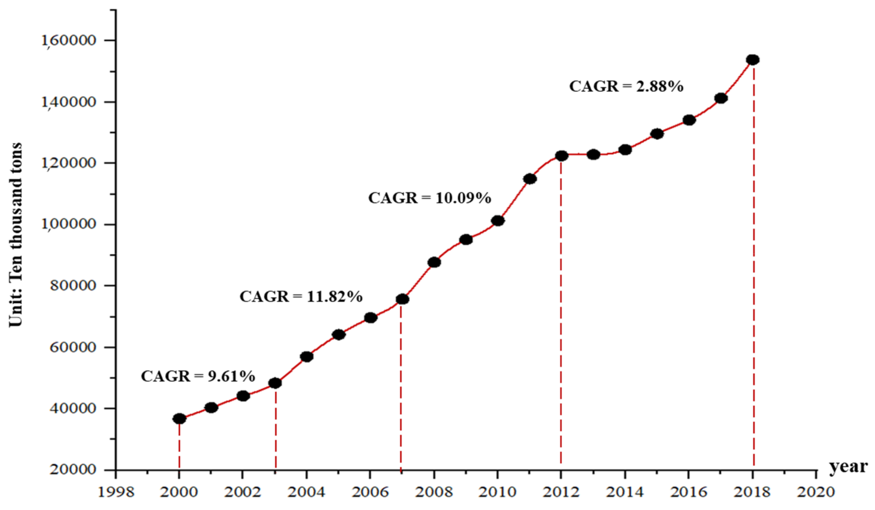
2, and the urban civil construction area accounted for 61.9%. In 2017, China’s total carbon emissions from buildings exceeded 2 billion tons of standard coal, which was about three times higher than the 668 million tons of carbon emissions in 2000, with an average annual growth rate of about 6.8% [1]. Statistics show that from 2000 to 2019, China’s urbanization rate rose from 36.2% to 60.6%, which is an increase in the urbanization rate of approximately 24.4%. By 2050, China’s urbanization rate may exceed 70%. With the acceleration of urbanization, a large amount of energy will be used in the building sector, and building energy consumption will continue to grow, which will be followed by continuous growth in carbon emissions.
In order to effectively solve the problem of carbon emissions, the Chinese government has implemented a series of policy measures. During the “Eleventh Five-Year Plan” period, the Chinese government made energy conservation a binding indicator for the first time and included it in the national economic and social development plan, and put forward the requirement that “the intensity of energy consumption in 2010 should be reduced by 20% compared with 2005.” During the “Twelfth Five-Year Plan” period, the Chinese government proposed for the first time a legally binding carbon dioxide emissions control target, that is, “a 17% reduction in the intensity of carbon dioxide emissions per 10,000 yuan during the period 2010–2015.” After the “Paris Agreement” came into effect, the Chinese government issued some energy-saving policies: “The carbon emission intensity in 2020 will be reduced by 18% compared to 2015”, and “achieve the emission reduction targets of carbon peak and carbon neutral by 2030 and 2060”. It can be seen that strengthening energy conservation and emissions reduction has become the focus of China’s efforts to achieve green and sustainable development.
In this context, Chinese universities and related scientific research institutions are vigorously carrying out research on building carbon emissions, and how to obtain basic data on building energy consumption has become the first problem to be solved in the research work. At present, China’s basic data sources for building energy consumption mainly include three methods: government statistical surveys, special surveys, and model calculations. Among them, the implementation agency of the government statistical survey method is the National Bureau of Statistics, which divides social and economic activities into four categories: primary industry, secondary industry, tertiary industry, and living consumption. It does not separate the construction sector separately, and energy consumption data is difficultly split. The implementation agency of the special survey method is the Ministry of Housing and Urban-Rural Development. According to the “Civil Building Energy Consumption Statistical Report System”, the energy consumption information of urban civil buildings and rural residential buildings is collected. The survey method adopts a combination of comprehensive survey and sample survey. Its data has not yet been disclosed to the public. Model calculation methods include the China Building Energy Consumption Model (CBEM) proposed by the Building Energy Consumption Model (CBEM) of Tsinghua University and the building energy consumption split model based on the energy balance sheet proposed by the Chinese scholar Professor Qing-Yi Wang. The two models currently use more calculation methods, but they can only obtain data on China’s total building energy consumption from a macro level, and cannot measure building energy consumption data on a detailed scale of cities and counties.
In addition, since there is no uniform method for China’s building carbon emissions accounting, which method is used to measure carbon emissions needs to be considered by the actual situation. Therefore, the input–output analysis method, emissions factor method, and life cycle method are often used in current research to calculate building carbon emissions.
The input–output method mainly analyzes the relationship between different sectors and different industries and estimates the direct and indirect carbon emissions of an industry from top to bottom in the form of an input–output table. Zhi-hui Zhang [2] used the input–output method to calculate the direct and indirect carbon emissions and carbon emissions correlation coefficients of buildings, which proved that carbon emissions have a significant pulling capacity. Xin Ju [3] used the emission factor method and the input–output method to calculate the carbon emissions of the construction industry and the consumption coefficient of the construction industry-related industries in China, and constructed a data calculation model for the construction industry-related carbon emissions. Jing Liu [4] built a building carbon emission data measurement model from the perspective of the entire industry chain based on the input–output method combined with energy statistics. Li-Yin Shen [5] used the input–output method based on the super-efficiency SBM model to measure and analyze the carbon emissions of residential buildings in China.
The emissions factor method is generally used to measure direct carbon emissions. This method needs to multiply the consumption of various types of energy with its carbon emissions factors to obtain the carbon emissions of each energy source, and then add the carbon emissions of each type of energy. After processing, the total value of energy carbon emissions can be obtained by summarizing. Jia Yang [6] calculated the carbon emissions of civil buildings in China’s provinces and cities using the emissions factor method based on energy consumption statistics. Fang-Wei Zhu [7] calculated the energy consumption and carbon emissions during the operation phase of public buildings in Wuhan using the carbon emissions factor method based on statistics and audit data. Meng-Jie Wang [8] measured the energy consumption of civil buildings in China’s urban areas based on statistical data and used the emissions factor method to obtain the total carbon emissions. Li-Chun-Yi Zhang [9] obtained relevant data of Tianjin Post and Telecommunications Apartment City through field research and questionnaire surveys and calculated the carbon emissions of residential buildings using the emissions factor method.
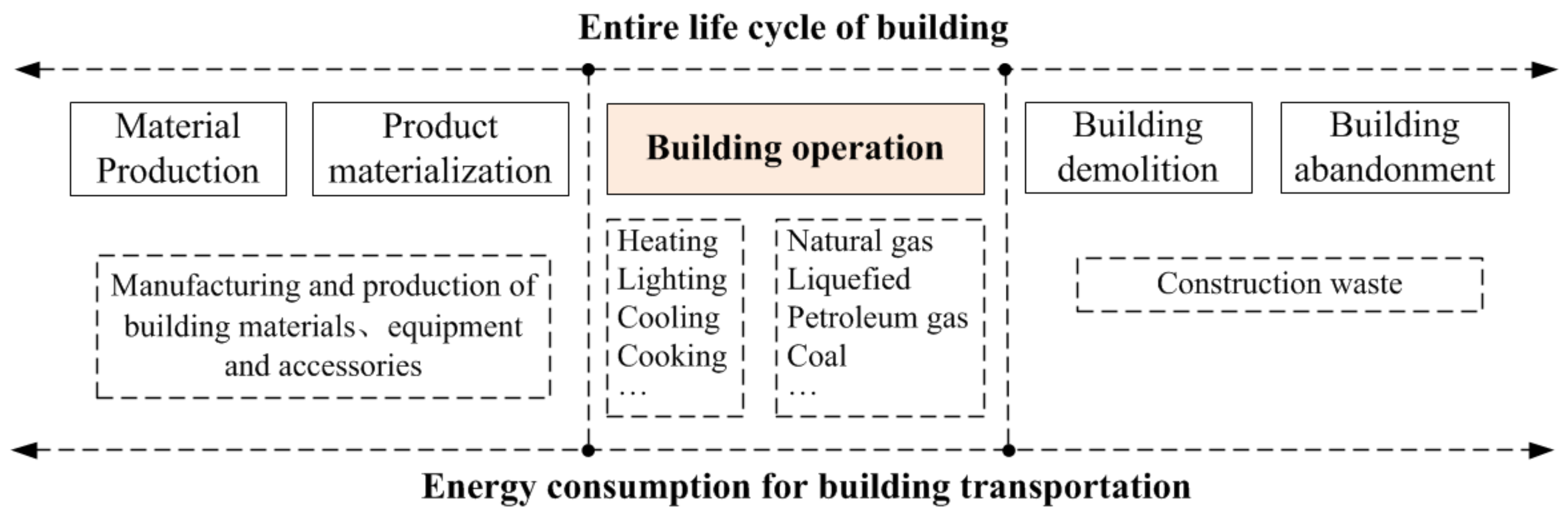
The whole life cycle method is a measurement method based on the whole life cycle theory, which is mainly used to estimate the carbon emissions of a certain product or a certain process during the whole life cycle. Xiao-Cun Zhang [10] analyzed the carbon emissions during the whole process of construction, operation, and demolition of buildings in China’s provinces based on energy statistics and using the life cycle method. Yi Chen [11] selected a single building project in Tianjin and analyzed the entire carbon emissions of the single building based on the building life cycle evaluation method and the emissions factor method. Xiao-Yun Zheng [12] used a villa project in Chongqing to calculate the total energy carbon emissions during the construction, operation, demolition, and abandonment phases of the building project using the whole life cycle method. In addition, Peng-Fei Cui [13] and Ze-Qiong Xie [14] also respectively measured the carbon emissions of the construction industry in China by stages based on the full life cycle method.
At present, many scholars [15,16,17,18] have carried out research work in the accounting method of carbon emissions, the spatial research of carbon emissions, and the relationship between lighting brightness and energy. Some achievements have been made, but there are limitations, as follows:
(1)
In the study of building carbon emissions accounting methods, domestic and foreign scholars mostly calculate building carbon emissions from both macro and micro levels. The basic data used for calculation are mostly split and calculated by using energy statistical yearbook data, and the spatial scale of calculation is also mostly at the national, provincial, and regional levels. In addition, the results of building carbon emissions obtained by different measurement methods also differ greatly. In view of this, remote sensing image data of lighting were introduced in this paper to extract lighting brightness values of different regions in Provinces, cities, and counties in China from 2000 to 2013, and the relationship model between lighting brightness values and building carbon emissions was established to further enrich the calculation methods and ideas of building carbon emissions.
(2)
In terms of measuring carbon emissions of building construction, the macro level is dominated by national and provincial scales of architecture, and the micro level is mainly composed of individual buildings. For the more detailed municipal and county scales, researching of carbon emissions of building is not perfect, and to some extent, the research also lacks the national, provincial, municipal, and county multi-level research of building carbon emission. So, it is unable to provide a more comprehensive and in-depth understanding of building carbon emissions in the field of construction. Therefore, based on the multi-regional building carbon emissions calculation model, this paper calculates the carbon emissions of urban civil buildings at the national, provincial, municipal, and county scales by using the lighting brightness values of provinces, cities, and counties.
On the whole, although Chinese scholars are constantly deepening their research on building carbon emissions, the lack of availability and refinement of basic building energy data not only provide insights into China’s provinces, cities, counties, and other carbon emissions at different scales. It also brings greater difficulties and greater limitations to the promotion of building energy conservation and emissions reduction. It can be seen that in order to effectively carry out research on building carbon emissions, it is urgent to introduce new data sources, broaden the research ideas of building carbon emissions, and provide data method support for research on building carbon emissions at a fine scale.
Light remote sensing images can characterize the intensity of human activities, and the data can be used to carry out research on human activities, carbon emissions estimation, and urban planning expansion. The main source of carbon emissions is human production and activities, and light brightness data can be used to indicate the strength of human activities. To a certain extent, there is also a strong correlation between night light data and carbon emissions.
This paper includes six parts: introduction, data collection, methodology, results, discussion, and conclusion. This paper aims to combine lighting remote sensing image data, energy statistics data, and geographic vector data, and to use panel data models to analyze the correlation between lighting brightness and building carbon emissions, constructing building carbon emissions data estimation models in eastern, central, and western regions of China. This model can estimate three spatial scales of carbon emissions from buildings, including province, city, and county, and analyze the characteristics of changes in building carbon emissions, providing a reference for formulating reasonable and sophisticating carbon emissions reduction policies.

2. Data Collection

2.1. Definition and Scope

2.1.1. Research Stage Division

The research object of this paper is the carbon emissions of urban civil buildings, including the carbon emissions of residential buildings and public buildings. The relevant concepts involved in the research are as follows:
Urban civil buildings: According to the nature of use, buildings can be divided into three types: civil buildings, industrial buildings, and agricultural buildings. This article takes civil buildings as the research object and divides them into two types: residential buildings, and public buildings.
Building carbon emissions: Carbon emissions in this article refer to carbon dioxide emissions (Figure 1). Building carbon emissions are derived from carbon emissions. Building carbon emissions can be divided into broad building carbon emissions and narrow building carbon emissions. The broad scope of building carbon emissions is defined as the carbon emissions during the entire life cycle of a building, including the building material production phase, building operation phase, and building demolition phase; the narrowly defined scope of building carbon emissions is the carbon emissions during the building operation phase. The carbon emissions of buildings in this article refer to the carbon emissions during the operation phase of buildings.

2.1.2. Research Area Division

The research scope of this article is the sum of the built-up areas of cities, counties, and organizational towns in 30 provinces and cities (excluding Xizang, Hong Kong, Macao, and Taiwan) in mainland China. There are great differences in factors such as social development and economic level among different regions, so there is a certain imbalance in the amount of carbon emissions generated between regions. In order to improve the rationality and accuracy of carbon emissions estimation, it is necessary to conduct regional analysis and estimation for different characteristics of carbon emissions. According to the level of social and economic development, this paper divides the selected 30 provinces and cities into three types of region [8]: eastern, central, and western regions (Table 1).

2.2. Data Collection and Calculation Flow

2.2.1. Building Carbon Emissions

The study area in this paper included 30 provinces and cities in mainland China, and the time series was from 2000 to 2017. The original energy consumption data came from the energy balance sheets of 30 provinces and municipalities in the “China Energy Statistical Yearbook” from 2000 to 2017, and the energy balance split model proposed by Qing-Yi Wang [19] was used to obtain basic building energy data. In this model, the energy consumption of different departments in the energy statistical yearbook needed to be split and converted according to a certain proportion and then summarized to obtain the energy consumption of urban civil buildings in various provinces and cities. Energy types included primary energy and secondary energy. The calculation method is as follows:
(1)
Transportation, warehousing, and postal industry: The energy consumption of this industry is included in buildings (including railway stations, terminal buildings, and post offices). The energy consumption is mainly electricity and heat. In addition, though the use of electric vehicles can generate electricity energy consumption, its proportion is so small that it can be ignored, and only the energy consumption of electricity and heat are calculated.
(2)
Wholesale, retail, accommodation, and catering: Most of this industry is buildings energy consumption, but it also includes energy consumption for transportation that needs to be deducted. Therefore, gasoline and diesel are calculated at the proportions of 5% and 65%, respectively.
(3)
Others: This industry includes the energy consumption of the tertiary industry other than (1) and (2) above, and it includes the energy consumption of transportation that needs to be deducted. Therefore, gasoline and diesel are calculated at the proportions of 5% and 65%, respectively.
(4)
Living consumption: This industry includes two parts: urban and rural areas. This article mainly studies urban living consumption in this industry, which includes all kinds of living consumption generated by residents, enterprises, institutions, government agencies, and the energy consumption of private transportation. Thus, it is not included in the consumption of gasoline in the industry, and the calculation ratio of diesel is 5%.
After obtaining basic building energy data, the carbon emission factor method [8] was used to calculate the carbon emissions of urban civil buildings in 30 provinces and municipalities in China. The calculation equation is as follows:
C = C i = δ i × e i
where C is the total carbon emissions of urban civil buildings in a province, e is the original energy consumption, δ is the carbon emissions factor, and i represents the type of energy.
The carbon emissions factors of various energy data were divided into the carbon emissions factors of primary energy (coal, gas, oil) and the comprehensive carbon emissions factors of secondary energy (electricity, heat). The carbon emissions factor of primary energy adopted national official data, and the carbon emissions factor of secondary energy was calculated according to the calculation formula of the energy balance sheet data.

2.2.2. Light Remote Sensing Image

The light remote sensing image data used in this paper came from the DMSP-OLS series of remote sensing satellites of the National Geophysical Data Center of the United States. The research time series was from 1992 to 2013, and 34 periods of light image data were obtained. Each image includes three types, specifically as follows: raw-avg-vis data, cloud-free coverages data, and the-cleaned-up-avg-vis data [20].
Light remote sensing image data include data indicators such as light brightness, light area, number of lights, and number of non-lights. The lighting attributes reflected by different lighting indicators are different. The light area index focuses on describing its distribution characteristics, and the light brightness index can simultaneously reflect the spatial distribution and three-dimensional characteristics of night lights. This paper selected the annual average light brightness value in the image data and constructed a panel data model of the building carbon emission.
After the light remote sensing image data were obtained, because the data of different years may come from different types of sensors, there were some problems in the stable light image obtained, as follows:
(a)
The DN value of the stable light image ranges from 0 to 63, so there may be saturated pixels with a DN value of 63, and it is most likely to exist in the central area of the city.
(b)
In the same year, there may be a certain difference between the total light DN value obtained by different sensors and the average light DN value.
(c)
In different years, abnormal changes may occur between the total light DN value obtained by the same sensor and the average light DN value.
Therefore, this article used ArcGIS 10.5 software to correct the original light data. The nighttime light image of China after correction is shown in Figure 2. The correction method is as follows:
Image reprojection, resampling, and cropping. Since the original extracted image data adopts the projection coordinate system of WGS84, in order to avoid the distortion of the pixel area of the light image, the original light image grid needed to be reprojected and converted to the Asia–Lambert–Conformal–Conic, using the NEAREST method to resample the lighting data into 1 km × 1 km and 0.5 km × 0.5 km grid sizes, and using the Chinese administrative division data as a mask, cropping and extracting the nighttime stable lighting image data in China.
Image mutual correction processing. In order to reduce the error of the DN value of the night light data of different sensors and different years, Elvidge [21] and others proposed a method for mutual correction of global night light data. After that, Liu [22], Zi-Yang Cao [23], and Yong-Xian Su [24] proposed a data correction method suitable for the constant target area of the Chinese regional lighting data under consideration of the actual situation in China. The specific processing methods are summarized as follows:
(a)
Since the economic development of Jixi City was relatively stable from 1992 to 2013, the city was selected as the target reference area based on the research of related scholars, and the light image of the F16 satellite in 2006 was used as the reference dataset.
(b)
The DN value of the F16 satellite in Jixi City in 2006 was extracted, and the quadratic regression model was used to regress it with the light DN value of other years. Correction parameters of a, b, and c were obtained. The calculation method is as follows:
D N 16 = a × D N 15 2 + b × D N 15 + c
(c)
Then the obtained mutual correction parameters a, b, and c were used to correct the acquired time series data. The calculation method is as follows:
D N = a × D N 0 2 + b × D N 0 + c
Based on the above, the correction regression model of the time series lighting data in China in this paper refers to the calculation parameters of Xing-Yong Zhou [25] to perform mutual correction on the image data in China.
The images will be fused during the year. In the same year, the light image data obtained may be obtained by multiple sensors. Since the detection performance of different sensors may be quite different, there are many differences in the DN value of the light brightness even in the image data obtained in the same year. Therefore, for remote sensing image data acquired from different sensors at the same time, correction processing for fusion within the year is required.
The light remote sensing image data obtained by different sensors in the same year are compared. If brightness information appears in only one image dataset at the same location, the pixel is defined as an unstable pixel. In addition, the DN value of the unstable pixel needs to be set to 0, and the DN value of the stable pixel in the image is set to the average value of the two images [26]; the calculation method is as follows:
D N ( n , i ) = 0
D N ( n , i ) = D N n , i a + D N n , i b / 2
where DN(n,i) represents the DN value of the pixel i in the n-th year after fusion within the year; D N n , i a , D N n , i b respectively represent the original DN value of the pixel i in the n-th year of satellite a and satellite b.
Image continuity correction between years. After performing the afore-mentioned three processing steps of mutual correction and intra-year fusion on the light image data, there may still be some inter-annual unstable pixels (the pixels have brightness information in the early images, but disappear in the later images), so it is necessary to perform inter-annual multi-sensor and multi-year continuity correction processing on the light image data. The calculation method is as follows:
D N n , i = D N n 1 , i ,     D N n 1 , i > D N n , i D N n , i ,             D N n 1 , i D N n , i          
where DN(n−1,i) and DN(n,i) are the DN value of the i-th pixel in the n−1-th and n-th year of the light image.

2.2.3. Availability of Light Remote Sensing Image

In recent years, the application of remote sensing image data has become more and more extensive, which has provided key basic support for many researches. Among all kinds of data obtained from remote sensing satellites, light remote sensing image data, as a good data source for inverting regional economic development and describing the impact of human production and activities, has many advantages that have been gradually highlighted. After the 1980s, the nightlight images have been widely used in the research of detection of human activities. For example, the nightlight images have been used to extend the monitoring of the spatial estimation of the regional economic development level, population, ecological environment, electric energy consumption, and other fields of human behaviors, providing strong support for the related studies.
Secondly, the nighttime light image not only has a larger monitoring range, but also a higher spatial and temporal resolution, which can detect the high intensity and low intensity nighttime light generated in a certain area. Many studies have verified that the main cause of carbon emissions is human production and activities, and nighttime light data can effectively reflect the intensity of human activities, and there is a strong correlation between light intensity and carbon emissions. Therefore, on the basis of the above research, this paper used lighting image data to build a relationship model between lighting image data and building carbon emissions, providing a new data source and a more detailed measurement method for carbon emissions data in the field of buildings.
In addition, the light remote sensing image data contain three different forms of light image data. The nighttime stable light image data can include areas with long-term light sources such as residential land in urban areas and residential land in towns. After removing the influence of background noise and other factors, such as the influence of light sources such as fire, moonlight, etc., the data is relatively accurate and highly usable.

3. Methodology

3.1. Research Premise and Hypothesis

In this paper, the premise of building a carbon emission estimation model using the brightness value of night lights was that the area with the greater brightness of light has the higher carbon emissions; that is, the area with the greater DN value of the light image data has the greater carbon emission value [27,28]. At the same time, it was assumed that there is a correlation between building carbon emissions and light brightness values as follows:
N C = a D N + b
where NC represents the estimated carbon emissions value, DN represents the light brightness value, and a and b represent the regression equation parameters.

3.2. Data Stationarity Test

Before constructing the panel data model, in order to avoid the phenomenon of false regression in the fitting of the established model, the stationarity test of the constructed panel dataset must be carried out to prove the validity of the model estimation. The stationarity test mainly includes two test methods: unit root test, and cointegration test. Among them, the unit root test is mainly used to test whether there is a unit root in the data; the co-integration test is mainly used to analyze whether there is a stable equilibrium relationship between factors. In addition, in order to eliminate the instability and heteroscedasticity that may exist in the time series during the inspection process, this paper processed the data in logarithm.
The unit root test methods include the same root unit test method (Levin–Lin–Chu (LLC)) and the different root unit root test method (Fisher-ADF). The first step of the unit root test is to start with the level sequence. If unit roots are found after the test, the first-order difference is performed, and the unit root test is continued; if the unit roots still exist after the test, the second or even higher order is performed After the difference, it is verified that the series is in a stationary state. If the null hypothesis that there is a unit root is rejected in both tests, the series is considered to be a stationary series [28]. If the unit root test is a single integer of the same order, the co-integration test can be used to analyze the stationarity of the data in the next step.
The co-integration test method adopts the co-integration test method based on the two-step method of Engel and Granger. Among them, the cointegration relationship used to test homogeneous panel data includes four statistics, namely the Panel V-Statistic, Panel rho-Statistic, Panel PP-Statistic, and Panel ADF-Statistic; and the cointegration relationship used to test heterogeneous panel data includes Group rho-Statistic, Group PP-Statistic, and Group ADF-Statistic [28,29]. If the data pass the cointegration test, the equation can be regressed, and more accurate results can be obtained.

3.3. Research Model Selection and Setting

Compared with the general regression model, the panel data model can not only solve the problem of sample size, but also can accommodate more information, allow large differences in data, eliminate the effect of multicollinearity, and improve the accuracy of estimation. Therefore, this paper builds a panel data model of night light brightness and carbon emissions and establishes an estimation model of urban civil building carbon emissions on the provincial scale of the eastern, central, and western regions. The specific steps of model establishment are as follows.

3.3.1. Panel Data Model Settings

Panel data models mainly include three types: constant coefficient models without individual influence (mixed regression model), constant coefficient models with individual influence (variable intercept model), and variable coefficient models with individual influence.
Mixed regression model. The mixed regression model has no individual influence and structural changes on the cross-section ( a i = a j = a , b i = b j = b ), so the model can be regarded as a simple accumulation of cross-sectional data. The regression form of the equation is as follows:
Y i t = a + b x i t Y + μ i t               i = 1 , 2 , 3 N ;   t = 1 , 2 , 3 T
Variable intercept model. The variable intercept model has only individual influences on the data cross-section, without structural changes ( a i a j , b i = b j = b ). In this model, the structural parameters of the variables on different cross sections are the same, but their intercept terms are different. Therefore, the difference in influence between individuals in the model can be represented by the difference in the intercept term ai (i = 1,2,3…N). If the individual influence of the model is constant, it is a fixed-effect variable-intercept model; if the individual influence of the model is a random variable, it is a random-effect variable-intercept model. The regression form of the equation is as follows:
Y I T = a i + b x i t + μ i t               i = 1 , 2 , 3 N ;   t = 1 , 2 , 3 T
Variable coefficient model. The variable coefficient model has individual influences and structural changes on the cross-section of the data. In this model, the change of individual influence is mainly represented by the intercept term ai (i = 1,2,3…N), and the structural change between individuals is represented by the coefficient vector bi (i = 1,2,3…N). The regression form of the equation is as follows:
Y i t = a i + b i x i t + μ i                               i = 1 , 2 , 3 N ;   t = 1 , 2 , 3 T

3.3.2. Choice of Panel Data Model

The first step of building a panel data model is to verify that the parameters ai and bi of the explained variable Yit are constant for all sample points and times in the model, and to further determine which estimation model should be selected for the selected sample data. In order to avoid large deviations in the selection of the model, it is usually necessary to use the F test for parameter testing, that is, the analysis of covariance method (analysis of covariance), and the test hypotheses are as follows:
Hypothesis 1 (H1).
b 1 = b 2 = = b N .
Hypothesis 2 (H2).
a 1 = a 2 = = a N ,   b 1 = b 2 = = b N .
Before starting the specific calculation steps of the model, it is necessary to calculate the residual sum of squares of the three models, namely, the residual sum of squares of the variable coefficient model (S1), the residual sum of squares of the variable intercept model (S2), and the mixed regression residual sum of squares model (S3). The specific calculation steps are as follows:
(1)
Under Hypothesis 2, it is necessary to test whether the F2 statistic obeys the F distribution of the corresponding degree of freedom. If the obtained F2 statistic value is less than the critical value under a certain level of significance (F2 < Fα), indicating that the tested sample meets the requirements of the mixed regression model, then accept Hypothesis 2; if F2 > Fα, continue to test the Hypothesis 1.
F 2 = S 3 S 1 / N 1 k + 1 S 1 / N T N k + 1   ~   F N 1 k + 1 ,     N T k 1
(2)
Under Hypothesis 1, it is necessary to test whether the F1 statistic also obeys the F distribution under the corresponding degree of freedom. If the obtained F1 statistic value is less than the critical value under a certain significance level (F1< Fα), indicating that the sample meets the requirements of the variable intercept model, then Hypothesis 1 is accepted; if F1 > Fα, it indicates that the sample meets the requirements of the variable coefficient model.
F 1 = S 2 S 1 / N 1 k + 1 S 1 / N T N k + 1   ~   F N 1 k + 1 ,     N T k 1
where N represents the number of sections, T represents the number of time series, and k represents the number of independent variables.
Generally, model effects are divided into fixed effects and random effects, and the choice of model effects can be determined using Hausmann’s test method. As related research has proved that the fixed-effect model can obtain relatively ideal results in most cases, this paper selected the fixed-effect model for estimation.

3.3.3. Construction of Carbon Emission Estimation Model

According to the model assumptions, after selecting and setting the panel data model, the relationship model between building carbon emissions and light brightness values at various scales in China can be established, and the parameter values a and b of the regression equations of 30 provinces in China can be calculated at the same time.
If there is a negative value when using the constructed panel data model to measure building carbon emissions, because the regional building carbon emissions cannot be negative, it needs to be set to zero to obtain a preliminary estimate of building carbon emissions [28]. At the same time, in order to improve the estimation accuracy of building carbon emissions at different scales, when using the panel data model for downscaling to analyze the building carbon emissions at the city and county level, it is necessary to use provincial carbon emissions data to obtain corrected city-level building carbon emissions data. The calculation method is as follows:
C = N C c t × S C N C n t
where c means a certain city; n means a province; t means a certain year; CC means the corrected building carbon emissions; NCct means the building carbon emissions estimated by the model; NCnt means the provincial level estimated by the model Building carbon emissions; and SC represents the provincial building carbon emissions derived from statistical data.

4. Results

4.1. Zoning Calculation Model of Building Carbon Emissions

4.1.1. Results of Stationarity Test

The unit root test results of the panel dataset of building carbon emissions and light brightness values are shown in Table 2. From the test results, in the Level value of the LLC test method, the building carbon emissions, light brightness, and urban population of the three regions rejected the null hypothesis at a significance level of 1%. However, the ADF-Fisher test method rejected the null hypothesis. According to the test results on the Level value, the building carbon emissions and light brightness both accepted the null hypothesis.
In order to further test the stationarity of the panel data, it was necessary to carry out the first-order difference unit root test on the panel data of the three regions. The final test results showed that in the LLC test and the ADF-Fisher test, the building carbon emissions and light brightness factors in the three regions rejected the null hypothesis at a significance level of 1%, indicating that the dataset is a first-order single integer stable Sequence data.
After the unit root test is performed on the established panel dataset, the result showed that the panel dataset is a first-order single integer. Therefore, the co-integration test analysis could be performed on the established panel dataset, and the test results are shown in Table 3.
In the case of homogeneous panel data, in the eastern region, Panel v-Statistic rejected the null hypothesis that there is no cointegration relationship at a significance level of 10%. Similarly, Panel rho-Statistic was also at a significance level of 5% and rejected the null hypothesis. In addition, Panel PP-Statistic and Panel ADF-Statistic both rejected the null hypothesis at the 1% significance level. In the central region, Panel v-Statistic, Panel PP-Statistic, and Panel ADF-Statistic all rejected the null hypothesis that there is no cointegration relationship at the 1% significance level, while the Panel rho-Statistic test accepted the null hypothesis. In the western region, Panel v-Statistic and Panel PP-Statistic both rejected the null hypothesis at the 1% significance level, Panel ADF-Statistic rejected the null hypothesis at the 5% significance level, and Panel rho-Statistic accepted the null hypothesis.
In the case of heterogeneous panel data, the test results of the eastern region and the central region were similar, and Group PP-Statistic and Group ADF-Statistic of the two regions were rejected at the significance level of 1% and 5%, respectively. So, there is no cointegration relationship. Group rho-Statistic accepted the null hypothesis; Group PP-Statistic and Group ADF-Statistic in the western region rejected the null hypothesis that there is no cointegration relationship at the 1% significance level, and Group rho-Statistic accepted the null hypothesis.
In general, the panel data of building carbon emissions and light brightness values in the eastern, central, and western regions passed the cointegration test at a certain level of significance, indicating that no matter which region, there is a long-term stable equilibrium relationship between the variables.

4.1.2. Results of Model Selection and Setting

In this paper, the method of covariance analysis was used to select the model form by calculating the F statistic. From the calculation results (Table 4), it can be seen that the statistics of the eastern region, F2 = 15.883 > F0.05 (24,156), rejected Hypothesis 2, and the statistics F1 = 0.397 < F0.05 (24,156) can be considered to accept Hypothesis 1. Therefore, the model form in the eastern region was chosen as the variable intercept model. Similarly, the statistics of the western region, F2 = 12.034 > F0.05 (20,132), rejected Hypothesis 2, and the statistics F1 = 0.542 < F0.05 (20,132) accepted Hypothesis 1. Therefore, the model form in the western region was also selected as the variable intercept model. For the central region, its statistics, F2 = 0.486 < F0.05 (10,72), accepted Hypothesis 2, so the model form of the central region was selected as a mixed regression model.
Based on the above selection results of model effects and model forms, this article used the generalized least squares method (GLS) to establish regression models under fixed effects for the three regions. The calculation results are as follows:
(1)
Eastern region: fixed-effect variable intercept model
The results of the fixed-effect variable-intercept model in the eastern region are shown in Table 5. From the test results, the model explanatory variable parameter was 1.0484 (0.0000), and the sample determination coefficient AR2 after model adjustment was 0.9973, indicating that the model had a high goodness of fit; the F statistic was 4886.83 (0.0000), passing the 1% significance level test and showing that the light data had significant explanatory power to the building carbon emission data; the DW statistic was 2.1526, indicating that the model did not have first-order autocorrelation. It can be seen that the fixed-effect variable-intercept model could better explain the relationship between night lights and building carbon emissions in the eastern region.
n N C i t = 1.0484 L n D N i t + b i t = 1.0484 L n D N i t + v i t 6.1871 i = 1 , 2 , 3 13               t = 1 , 2 , 3 14
where NC represents the estimated carbon emission value of the i-th province in year t; DN represents the light brightness value of the i-th province in year t; Ln represents the log of a variable; b and v respectively represent the model intercept term and the fixed impact value.
(2)
Middle region: mixed regression model
The results of the mixed regression model in the central region are shown in Table 6. From the model test results, the model explanatory variable parameters were 0.8773 (0.0000), the intercept term was −4.2414, and the sample determination coefficient AR2 after model adjustment was 0.9377, indicating that the mixed regression model had a better fit; the F statistic value was 1250.350 (0.0000), passing the 1% significance level test, indicating that the light data in the central region had a significant explanatory power for building carbon emissions; the DW statistic was 1.3403, indicating that the model did not have first-order autocorrelation. It can be seen that the hybrid regression model could better explain the relationship between night lights and building carbon emissions in the central region.
L n N C i t = 0.8773 L n D N i t + b = 0.8773 L n D N i t 4.2414 i = 1 , 2 , 3 6               t = 1 , 2 , 3 14
where NC represents the estimated carbon emission value of the i-th province in year t, DN represents the light brightness value of the i-th province in year t, Ln represents the log of a variable, and b represents the intercept term of the hybrid regression model.
(3)
Western region: fixed-effect variable-intercept model
The results of the fixed-effect variable-intercept model in the western region are shown in Table 7. From the model test results, the model explanatory variable parameter was 0.3645 (0.0000), and the sample determination coefficient AR2 after model adjustment was 0.9977, indicating that the goodness of fit of the model was relatively high; the F statistic was 6056.08 (0.0000), passing the 1% significance level test, showing that the light data had significant explanatory power to the building carbon emission data; the value of the DW statistic was 2.0199, indicating that the model did not have first-order autocorrelation. It can be seen that the fixed-effect variable-intercept model (16) could better explain the relationship between the brightness of the lights at night and the carbon emissions of buildings in the western region.
L n N C i t = 0.3645 L n D N i t + b i t = 0.3645 L n D N i t + v i t + 2.2189 i = 1 , 2 , 3 11                   t = 1 , 2 , 3 14
where NC represents the estimated carbon emission value of the i-th province in year t, DN represents the light brightness value of the i-th province in year t, Ln represents the log of a variable, b and v respectively represent the model intercept term and the fixed impact value.

4.1.3. Result of Accuracy Test

There are two main ways to evaluate the accuracy of carbon emissions estimation: one is to examine the correlation between the building carbon emission statistics and the building carbon emission simulation value, and to use the determination coefficient AR2 for testing; the second is to examine the building carbon emission statistics and the building carbon emission statistics. The error method of the emission simulation value is judged by using the root mean square error (RMSE) [29,30].
Taking account into the availability of building carbon emission statistics, this paper selected the building carbon emissions model estimation data and carbon emissions statistics data in 2000, 2005, 2008, and 2012 for accuracy evaluation. As can be seen from Figure 3, the coefficients of determination AR2 of the simulated and statistical values of the building carbon emission models in 2000, 2005, 2008, and 2012 were 0.7975, 0.9082, 0.9584, and 0.7636, respectively, and the RMSE values of the root mean square error were 14642, 467.10, 974.26, and 1981.68 (ten thousand tons), respectively. It can be seen that the degree of fit between the carbon emissions of urban civil buildings and the building carbon emissions statistics obtained by using the panel data model was good, and the panel data model had good accuracy. Therefore, it can be used to estimate the carbon emissions of buildings at different scales.

4.2. Temporal and Spatial Evolution Characteristics of Building Carbon Emissions

According to the overall calculation results (Figure 4), the growth trend of domestic urban civil building carbon emissions from 2000 to 2017 could be roughly divided into four stages: the average annual growth rate of civil building carbon emissions from 2000 to 2003 was about 9.61%. From 2003 to 2012, the growth rate of carbon emissions from urban civil buildings gradually increased; from 2003 to 2007, the average annual growth rate was about 11.82%; from 2007 to 2012, the average annual growth rate was 10.09%. The total amount of carbon emissions from buildings produced in 2003 was about 467,934,700 tons. By 2012, carbon emissions from urban civil buildings had increased to 1255936 million tons. After 2012, the growth rate of carbon emissions gradually slowed down. By 2017, the total carbon emissions from buildings were approximately 1142.8715 million tons, with an average annual growth rate of approximately 2.88%.

4.2.1. Changes in Building Carbon Emissions at Multiple Scales

Changes in carbon emissions from provincial and municipal buildings were examined. It can be seen that the areas with higher carbon emissions from civil buildings in provincial cities and towns were mainly located in the northern and eastern regions, and there was a trend of gradual expansion inland, such as Inner Mongolia. The total building carbon emissions of the autonomous region from 2000 to 2015 gradually changed from a medium level to a high level. Areas with low carbon emissions from urban civil buildings were mainly distributed in the northwest and southwest regions with low economic levels, including Qinghai, Gansu, Xinjiang Uygur Autonomous Region, Yunnan, and Guangxi Zhuang Autonomous Region.
Changes in carbon emissions from county-level buildings were also examined. According to the building carbon emission calculation model, this paper estimated the growth rate of carbon emissions from civil buildings in county-level cities and towns from 2000 to 2013, and it divided the growth trend of building carbon emissions in 2778 county-level regions across the country into slow growth, slower growth, medium-speed growth, relatively fast growth, and fast growth five types.
The results showed that there were a total of 1054 county-level regions in the country that were of slow growth and slower growth, and they were concentrated in the northwest and southwest regions of economically underdeveloped areas, accounting for about 37.91%; in terms of the number of medium-speed growth regions, there were 1467, and they were mainly distributed in inland areas and developed coastal areas, accounting for about 52.81%. In addition, the number of regions with faster growth rates and the number of regions with rapid growth rates were 248 and 9, respectively, accounting for 8.93% and 0.32%, respectively. The distribution was relatively loose, showing the characteristics of sporadic distribution in the southeast coastal and northern regions. Preliminary findings indicate that there is a close relationship between the growth rate of domestic urban civil construction carbon emissions and the regional economic level.

4.2.2. The Spatiotemporal Direction of Building Carbon Emissions at Multiple Scales

Distribution directionality refers to the outline and dominant direction of the spatial distribution of a certain attribute given to a region. Standard Deviational Ellipse (SDE) is a statistical method in the discipline of geography. It can analyze the directional characteristics of the spatial distribution of a certain attribute in a region, and at the same time, it can quantitatively explain the center and directional characteristics of its spatial distribution from a global perspective [31,32,33,34,35].
This paper introduces the directional analysis method in geography into the study of building carbon emissions and uses ArcGIS to analyze the directional changes in the spatial distribution of carbon emissions from urban civil buildings at different scales in China. By comparing the difference in the area covered by the standard deviation ellipse in different years, and the changes in the X-axis and Y-axis, we further analyze and describe the temporal changes and direction trends of carbon emissions from urban civil buildings in the time series.
The temporal and spatial directions of carbon emissions from provincial buildings were examined. From 2000 to 2017, the ellipse generation area of the carbon emissions of civil buildings in provincial cities and towns gradually increased, indicating that the scope of influence of the carbon emissions of urban civil buildings was gradually expanding. The oblateness of an ellipse can be used to express the clarity of the direction and the degree of centripetal force. From the results of the oblateness of the generated ellipse, the oblateness of the ellipse at the provincial scale gradually decreased from 2001 to 2017, indicating that the direction of carbon emissions in 2017 was clearer than that in 2016 and other years.
From the perspective of the change of the spatial direction angle, the direction angle decreased from 72.1216 to 71.1995, and the direction of the ellipse gradually shifted to the east and north. Looking at the changes in the X-axis and Y-axis of the ellipse, the long axis dropped from 12.8873 in 2011 to 12.8116 in 2017, a small decrease, and the short axis rose from 9.1856 in 2011 to 9.2691. The fluctuation of the long and short axes of the ellipse was smaller. It can be seen that the total amount of carbon emissions from buildings at the provincial level was increasing year by year, but its spatial distribution pattern was relatively stable, and the east–west direction had a greater influence than the north–south direction.
The temporal and spatial directions of carbon emissions from municipal buildings were examined. From 2001 to 2013, the elliptical area of carbon emissions from civil buildings at the municipal level showed a wave-shaped change trend. The overall elliptical area did not change much, and the area of elliptical were between 463 and 464. From the perspective of the oblateness of the generated ellipse, the oblateness of the ellipse from 2001 to 2013 showed a gradual decrease. The specific manifestation was that the oblateness of the ellipse was about 0.3127 in 2001, and the oblateness of 2013 was gradually reduced to 0.3053, indicating the direction of carbon emission and the degree of centripetal force were increasing year by year. From the perspective of the change of the spatial direction angle, the direction angle gradually decreased from 88.3454 to 87.5334, and the ellipse direction still reflected the shift to the east and north direction, which was consistent with the results of the provincial-level direction angle change.
From the change of the long axis of the ellipse X and Y, the lengths of the long axis and the short axis in 2001 were 14.6714 and 10.0861, respectively, and the lengths of the long axis and the short axis were 14.5675 and 10.1207, respectively in 2013. The specific manifestation is that the length of the long axis was present. There was a slight downward trend; the length of the short axis showed a slight increase, and the change trend of the long and short axis of the ellipse was consistent with the provincial change, which shows that the results of changes in building carbon emissions at the municipal and provincial levels were consistent, and the spatial distribution direction also showed a gradual shift to the northeast.
The spatial and temporal directions of county-level building carbon emissions were examined. From 2001 to 2013, the change trend of the elliptical area of carbon emissions from civil buildings at the county level was similar to that of the municipal ellipse, showing a wave-shaped change trend as a whole. From the perspective of the flattening rate of the generated ellipse, the flattening rate of the ellipse from 2001 to 2013 showed a gradual decrease. The specific manifestation is that the carbon emission elliptical flattening rate of county-level buildings in 2001 was 0.3097, and the elliptical flattening rate increased to 0.3103 in 2005. Since then, the ellipse flatness showed a decreasing trend, and by 2013 its ellipse flatness was about 0.3083. Judging from the changes in the elliptical oblateness of carbon emissions from county-level buildings, the directionality and centripetal force were still showing an increasing trend, which was consistent with the analysis results at the provincial and municipal levels. From the perspective of the change of the spatial direction angle, from 2001 to 2013, the spatial direction angle gradually increased from 81.3830 to 81.5170 in 2007, and then gradually decreased to 80.0517 in 2013. The change in the direction angle of the ellipse was consistent with the provincial and municipal level. The analysis results were consistent, gradually shifting to the east and north.
On the whole, the standard deviation ellipse area of building carbon emissions at the provincial, municipal, and county levels in China was not much different, and the performance results on different scales were relatively consistent, indicating that the spatial distribution pattern of building carbon emissions at each scale was relatively stable. The elliptical distribution direction also showed a trend of changing to the northeast.

5. Discussion

In view of the insufficient availability and low level of refinement of the basic data sources of China’s building carbon emissions, this article explores a method for measuring carbon emissions from buildings in China at multiple scales. This study used Chinese civil buildings as the object and combined building carbon emissions data with light remote sensing image data to construct a building carbon emissions measurement model for three regions in eastern, central, and western China; after that, based on the model, the provinces, cities and counties of China were calculated. Building carbon emissions at three scales of province, city, and county were determined using the SDE method to explore the temporal and spatial evolution characteristics of building carbon emissions at the provincial, city, and county scales, and suggestions were put forward for the implementation of building carbon emission reduction.

5.1. Sources of Basic Data on Building Carbon Emissions

As an information product of urban development, energy data represent an important basis for measuring carbon emissions, analyzing energy-saving potential, and formulating energy-saving goals, and provide key information support for the effective development of energy-saving work. However, at present, there are still some problems that need to be solved in the basic data of carbon emissions in the Chinese construction sector.
The availability of basic building carbon emissions data needs to be improved. China’s existing basic data sources for building carbon emissions estimation are mainly two statistical systems, namely the National Bureau of Statistics, and the Ministry of Housing and Urban–Rural Development. The first is the statistics source of the National Bureau of Statistics. In the energy balance sheet of the “China Energy Statistical Yearbook”, although various energy consumption data cover the seven major industries including the construction industry, they do not directly cover the energy consumption data during the operation phase of the building. The availability and use of data are limited due to insufficient performance, and most existing studies still calculate building energy consumption and carbon emissions by splitting the energy balance sheet. The second is the statistics source of the Ministry of Housing and Urban–Rural Development. The statistical system mainly uses the civil building energy resource data monitoring platform constructed in the early stage to obtain the consumption data of different types of energy produced by various buildings. Although the data obtained by this method are more authoritative, they have not been disclosed to the outside world, and the data sharing is insufficient.
The level of refinement of basic building carbon emissions data urgently needs to be deepened. At present, the measurement method used in most studies is to obtain building energy consumption by splitting the energy balance sheet and then using the carbon emissions factor method to calculate the carbon emissions of the building. However, the spatial granularity of the building carbon emissions data obtained by this method is relatively large, and only national- and provincial-level building carbon emissions data can be obtained. The more detailed spatial-scale data such as municipal and county levels cannot be obtained. In addition, China’s construction sector still lacks basic and detailed data, such as carbon emissions data for different building types, carbon emissions data for different energy types, and carbon emissions data for different end uses (heating, lighting, etc.).
At present, China does not have direct access to building energy consumption data in the construction sector. It can only obtain building carbon emissions data by using statistical data based on model predictions, split calculations, etc., and in terms of data availability and granularity as well as accuracy, there are certain problems, and it is urgent to introduce new research ideas and methods.

5.2. Limitations of this Research

This work has some limitations which need to be solved.
(1)
The data used in this study can be divided into two types: one is the official data source that has a greater impact on the results of this paper, such as light remote sensing image data and geographic vector data. This type of data is obtained through official channels and large-scale survey statistics. It is currently the most reliable type of data and can also support the development of this research. The second type of data is also a key data source in the research, but there is no official data acquisition channel, such as building carbon emissions data. For this type of data, we conducted a large-scale literature survey and research in the early stage, and obtained relevant data from many studies. However, it is undeniable that China currently lacks official data on carbon emissions in the construction sector, especially data on more detailed spatial scale types. In the future, more attention should be paid to the research of this aspect of data.
(2)
This article mainly analyzes the correlation between building carbon emissions and lighting values and builds a panel data model for building carbon emissions data and lighting values. Since the analysis is mainly carried out on the provincial scale in this study, although the corrective calculation formula has been proposed in the previous article, there will still be some errors when using this model to calculate the carbon emissions of buildings at the city and county levels. In the future, with the gradual establishment of related big data platforms such as building energy conservation in various provinces and cities in China, building carbon emission data can be used to carry out more refined research work. In addition, other types of data can also be introduced to construct building carbon emission estimation models under different spatial scales.

6. Conclusions

6.1. Key Findings

Based on the results and discussion above, the key findings of this article are presented as follows:
(1)
There is a balanced and stable relationship between building carbon emissions and lighting values. After the stability test of the panel dataset of building carbon emissions and lighting brightness, the panel data of the eastern, central and western regions all passed the significance test, and they are all stable sequences of order 1 single integer, indicating that in terms of building carbon, there is a long-term balanced and stable relationship between emissions and light brightness. In addition, after the accuracy test of the constructed building carbon emissions zoning measurement model, the results of the determination coefficient AR2 between the statistical value and the simulated value and the root mean square error RMSE all passed the test, indicating that the building obtained using the panel data model. Carbon emissions and carbon emissions statistics have a good fit, and the model has good accuracy, which can be used to estimate building carbon emissions at different scales.
(2)
Although the total carbon emissions of civil buildings in China are showing an increasing trend, their average annual growth rate is gradually slowing down. From 2000 to 2003, the average annual growth rate of carbon emissions from buildings in China was about 9.61%. After 2003, the growth rate of building carbon emissions gradually accelerated. The average annual growth rate from 2003 to 2007 was approximately 11.82%, and the average annual growth rate from 2007 to 2012 was 10.09%. After 2012, the growth rate of carbon emissions gradually slowed down. By 2017, the total carbon emissions of civil buildings in China were about 1412.8715 million tons, with an average annual growth rate of only 2.88%.
(3)
The spatial and temporal development directions of building carbon emissions at the three scales of provinces, cities, and counties in China are basically the same, all showing a trend of shifting to the east. From the results of the spatial and temporal direction analysis of building carbon emissions, the standard deviation ellipse area of building carbon emissions at the provincial, municipal, and county levels in China is not much different, and the performance results on different scales are relatively consistent, indicating that in terms of the building carbon on all scales, the spatial distribution pattern of emissions is relatively stable, and the elliptical distribution direction as a whole shows a trend of change toward the east.

6.2. Policy Recommendation

In view of the results, the following recommendations are presented:
The industrial structure of eastern and central provinces in China is mainly labor-intensive and light industry. Factors such as building area, electrical appliances ownership, and consumption level have a greater impact on the carbon emissions of buildings in the region. Therefore, the emissions reduction strategy in this region can focus on promoting the application of energy-saving technologies and improving the efficiency of building end-use energy. Building energy-saving technology directly affects the energy-saving effects of buildings. The government should establish a sound building technology research policy, incorporate relevant research projects into the management of building technology plans, and do a good job in the research and development of key energy-saving technologies in the field of construction, focusing on key points such as urban planning, urban construction, building structure, building energy efficiency, and building information construction. Special issues could be included diversified investment in construction technology innovation. Second, we should speed up the transformation and promotion of building energy-saving scientific and technological achievements, and make full use of energy-saving product identification and scientific and technological certificate certification promotion to promote the application of energy-saving materials and products in the construction field, and further enhance the effect of building energy-saving. In addition, the government should also pay attention to the energy efficiency of end-use energy products, and meet the energy needs of residential users of buildings with low energy consumption. For example, in the field of building refrigeration, clean energy can be used to replace harmful refrigerants such as fluorine. At the same time, new technologies such as indirect evaporative refrigeration, absorption refrigeration, and liquid desiccants can be applied to avoid problems such as refrigerant leakage. At the same time, attention should be paid to the recovery of refrigerants to promote the market for building equipment and appliances such as air conditioners and refrigerators is shifting to more efficient production technologies, which promotes the market development of high-efficiency products and equipment.
The industrial structure of the provinces in the western and northern regions of China is mostly heavy industry, and central heating is mostly used in buildings. The energy use structure and energy efficiency have a greater impact on the carbon emissions of buildings in the region. Therefore, emission reduction strategies in this region can focus on introducing clean energy-saving technologies and improving energy efficiency. The government can start from the heating end in the short term to improve the heating efficiency of buildings. One is to improve the insulation and airtightness of buildings, improve the performance of building envelopes (such as the insulation value of windows) and building energy performance standards and building heating energy requirements, and rationally design building indoor heating and ventilation structures. The second is the use of efficient and concise heating systems, the design of urban underground comprehensive pipe corridors, and the use of high-temperature circulation and straight-line laying methods to reduce the heat loss rate of the heating transmission and distribution network and improve the energy efficiency of central heating. Although the region consumes a lot of resources such as coal, it is rich in clean resources such as solar energy, geothermal energy, and wind energy. From the perspective of medium-term development, the region can use its resource advantages to introduce high-efficiency and clean energy in building heating and cooling and increase the use of clean energy such as natural gas and electricity; reduce boiler use and increase use of solar energy equipment; and promote combined heat and power mode, recovering the waste heat of power generation and applying it to heating, gradually optimizing the energy structure.

Author Contributions

Conceptualization, T.Y.; methodology, T.Y. and Z.C.; software, T.Y. and Y.W.; formal analysis, T.Y. and J.L. (Jing Liu); investigation, T.Y. and J.L. (Jing Liu); data curation, J.L. (Jiahui Luan), H.H. and Z.W.; supervision, T.Y.; project administration, T.Y. and H.M.; visualization, Z.C., Y.W. and H.H.; validation, J.L. (Jing Liu) and H.M.; writing—original draft, T.Y.; writing—review and editing, T.Y. and J.L. (Jing Liu). All authors have read and agreed to the published version of the manuscript.

Funding

This research received no external funding.

Institutional Review Board Statement

Not applicable.

Informed Consent Statement

Not applicable.

Data Availability Statement

Not applicable.

Conflicts of Interest

The authors declare no conflict of interest.

Abbreviations

AbbreviationFull Name
CBEMChina Building Energy Consumption Model
DMSPDefense Meteorological Satellite Program
OLSOperational Linescan System
DNDigital Number
LLCLevin–Lin–Chu
ADFAugmented Dickey Fuller
PPPhillips and Perron
RhoSpearman’s Rank Correlation
GLSGeneralized Least Squares Method
DWDurbin Watson
RMSEThe Root Mean Square Error
SDEStandard Deviational Ellipse

References

  1. M. China Building Energy Efficiency Annual Development Research Report; Building Energy Conservation Center of Tsinghua University: Beijing, China, 2020. (In Chinese)
  2. Zhang, Z.; Liu, R. Carbon emission accounting of construction industry based on input-output analysis. J. Tsinghua Univ. Sci. Technol. 2013, 53, 53–57. (In Chinese) [Google Scholar]
  3. Ju, X. Measurement and Influencing Factors of Provincial Carbon Dioxide Emissions in China’s Construction Industry. Master’s Thesis, Tianjin University, Tianjin, China, 2016. (In Chinese). [Google Scholar]
  4. Liu, J. Research on the Measurement Method and Emission Reduction Policy of China’s Construction Industry Chain from the Perspective of Carbon Footprint. Master’s Thesis, Beijing Jiaotong University, Beijing, China, 2018. (In Chinese). [Google Scholar]
  5. Shen, L.; Zhu, M.; Wu, Y. Carbon efficiency measurement of residential buildings in China. J. Urban Issues 2019, 10, 53–62. (In Chinese) [Google Scholar]
  6. Yang, J. Research on the Difference of Energy Consumption and Carbon Emission of Urban Residential Buildings in China. Master’s Thesis, Chongqing University, Chongqing, China, 2016. (In Chinese). [Google Scholar]
  7. Zhu, F.-w.; Zhang, C.-z.; Chen, Y.-h. Research on carbon emission of public buildings in Wuhan. Heat. Vent. Air Cond. 2018, 48, 79–84. (In Chinese) [Google Scholar]
  8. Wang, M. Regional Differences and Influencing Factors of Carbon Emissions from Urban Buildings in China. Master’s Thesis, Beijing Jiaotong University, Beijing, China, 2019. (In Chinese). [Google Scholar]
  9. Zhang, C.; Sun, Q.; Wu, H. The relationship between carbon emission and residential environment in urban residential areas: A Case study of Cheng-nan Jia-yuan, Xinyuan Village, Tianjin. Build. Energy Conserv. 2020, 48, 93–107. (In Chinese) [Google Scholar]
  10. Zhang, X. Research on Quantitative Analysis and Calculation of Building Carbon Emission and Evaluation Method of Low-Carbon Building Structure. Master’s Thesis, Harbin Institute of Technology, Harbin, China, 2018. (In Chinese). [Google Scholar]
  11. Chen, Y.; Zhang, J.; Song, C. Research on carbon emission of green Building in its life cycle -- A Case study of New business Housing project of Tianjin Architectural Design Institute. City 2019, 226, 77–81. (In Chinese) [Google Scholar]
  12. Zheng, X. Life cycle carbon emission of prefabricated buildings based on LCA: A case study of a light steel prefabricated integrated villa in Chongqing. Build. Econ. 2019, 40, 107–111. (In Chinese) [Google Scholar]
  13. Cui, P. Research on Phasing Emission Reduction Strategy of Construction Industry Based on Life-Cycle Carbon Emission Measurement. Master’s Thesis, Taiyuan University of Science and Technology, Taiyuan, Shanxi, 2019. (In Chinese). [Google Scholar]
  14. Xie, Z. Research on Calculation, Prediction and Evaluation of Consumer Carbon Emission in Guangdong Province. Master’s Thesis, South China University, of Technology, Guangzhou, China, 2018. (In Chinese). [Google Scholar]
  15. Wang, R.; Zhang, H. Spatial distribution and influencing factors of carbon emissions in County-level cities of China based on urbanization. Prog. Geogr. 2021, 40, 1999–2010. (In Chinese) [Google Scholar] [CrossRef]
  16. Hu, M. Spatial Pattern and Influencing Factors of Carbon Emissions at County Level in China. Master’s Thesis, Lanzhou University, Lanzhou, China, 2021. (In Chinese). [Google Scholar]
  17. Li, X. Research on Carbon Emission Trading Mechanism of Urban Public Buildings in China. Master’s Thesis, Beijing Jiaotong University, Beijing, China, 2021. (In Chinese). [Google Scholar]
  18. Wang, Y. Spatial-Temporal Differences and Influencing Factors of Carbon Emission Intensity in China’s Construction Industry. Master’s Thesis, Harbin Normal University, Harbin, China, 2021. (In Chinese). [Google Scholar]
  19. Wang, Q. Research on statistics and Calculation of Building energy consumption in China. Energy Sav. Environ. Prot. 2007, 8, 9–10. (In Chinese) [Google Scholar]
  20. Ji, X. Simulation, Pattern and Mechanism of Carbon Emission from Energy Consumption in Bohai Rim Region Based on Night Light Data. Master’s Thesis, Northwest Normal University, Lanzhou, China, 2017. (In Chinese). [Google Scholar]
  21. Elvidge, C.D.; Baugh, K.E.; Kihn, E.A.; Kroehl, H.W.; Davis, E.R.; Davis, C.W. Relation between satellite observed visible near infrared emissions, population, economic activity and electric power consumption. Int. J. Remote Sens. 1997, 18, 1373–1379. [Google Scholar] [CrossRef]
  22. Liu, Q.; Wu, R.; Zhang, W.; Li, W.; Wang, S. The varying driving forces of PM2.5 concentrations in Chinese cities: Insights from a geographically and temporally weighted regression model. Environ. Int. 2020, 145, 106168. (In Chinese) [Google Scholar] [CrossRef] [PubMed]
  23. Cao, Z.; Wu, Z.; Kuang, Y.; Hang, N. Calibration and application of DMSP/OLS nighttime light image in China. J. Geo-Inf. Sci. 2015, 17, 1092–1102. (In Chinese) [Google Scholar]
  24. Su, Y. Carbon Emissions from Energy Consumption in China Based on DMSP/OLS Nighttime Light Data. Ph.D. Thesis, Graduate University of Chinese Academy of Sciences (Guangzhou Institute of Geochemistry), Guangzhou, China, 2015. (In Chinese). [Google Scholar]
  25. Chow, X. Estimation and Spatial-Temporal Distribution of Carbon Emissions from Energy Consumption Based on Night Light Data in Guangdong Province. Master’s Thesis, Chengdu University of Technology, Chengdu, China, 2018. (In Chinese). [Google Scholar]
  26. Han, J.; Meng, X.; Liang, H.; Cao, Z.; Dong, L.; Huang, C. An improved night-light based method for modeling urban CO2 emissions. Environ. Model. Softw. 2018, 107, 307–320. (In Chinese) [Google Scholar] [CrossRef]
  27. Wu, M. Spatial-Temporal Characteristics and Influencing Factors of Carbon Emission Intensity in China’s Construction Industry Based on GTWR Model. Master’s Thesis, Chang’an University, Xi’an, China, 2019. (In Chinese). [Google Scholar]
  28. Shi, K. Spatial-Temporal Dynamics and Influencing Factors of Carbon Emissions in China from a Multi-Scale Perspective. Ph.D. Thesis, East China Normal University, Shanghai, China, 2017. (In Chinese). [Google Scholar]
  29. Wei, L.; Zhang, Y.; Li, Q. Ecological differentiation of China based on standard deviation ellipse. Ecol. Econ. 2020, 36, 176–181. (In Chinese) [Google Scholar]
  30. Zhao, J.; Ji, G.; Yue, Y.; Lai, Z.; Chen, Y.; Yang, D.; Yang, X.; Wang, Z. Spatio-temporal dynamics of urban residential CO2 emissions and their driving forces in China using the integrated two nighttime light datasets. J. Appl. Energy. 2019, 235, 612–624. [Google Scholar] [CrossRef]
  31. Xiao, H.; Ma, Z.; Mi, Z.; Kelsey, J.; Zheng, J.; Yin, W.; Yan, M. Spatio-temporal simulation of energy consumption in China’s provinces based on satellite night time light data. Appl. Energy 2018, 231, 1070–1078. [Google Scholar] [CrossRef]
  32. Lu, H.; Liu, G. Spatial effects of carbon dioxide emissions from residential energy consumption: A county-level study using enhanced nocturnal lighting. Appl. Energy 2014, 131, 297–306. [Google Scholar] [CrossRef]
  33. Shi, K.; Chen, Y.; Yu, B.; Xu, T.; Chen, Z.; Liu, R.; Li, L.; Wu, J. Modeling spatiotemporal CO2 (carbon dioxide) emission dynamics in China from DMSP-OLS nighttime stable light data using panel data analysis. Appl. Energy 2016, 168, 523–533. [Google Scholar] [CrossRef]
  34. Shi, K.; Chen, Y.; Li, L.; Huang, C. Spatiotemporal variations of urban CO2 emissions in China: A multiscale perspective. Appl. Energy 2018, 211, 218–229. [Google Scholar] [CrossRef]
  35. Yang, D.; Luan, W.; Qiao, L.; Pratama, M. Modeling and spatio temporal analysis of city-level carbon emissions based on nighttime light satellite imagery. Appl. Energy 2020, 268, 114696. [Google Scholar] [CrossRef]
Figure 1. Definition of research indicators.
Sustainability 14 02269 g001
Figure 2. Correction of light images at night in China: (a) 2002, (b) 2004, (c) 2006.
Sustainability 14 02269 g002
Figure 3. Diagram of carbon emission accuracy evaluation: (a) 2000, (b) 2005, (c) 2008, (d) 2012.
Sustainability 14 02269 g003
Figure 4. Carbon emissions trend of urban buildings.
Sustainability 14 02269 g004
Table 1. Regional division results.
TypeProvinceQuantity
Eastern regionLiaoning; Jilin; Heilongjiang; Beijing; Tianjin; Hebei; Shandong; Shanghai; Jiangsu; Zhejiang; Fujian; Guangdong; Hainan13
Central regionShanxi; Henan; Anhui; Jiangxi; Hubei; Hunan6
Western regionShanaxi; Gansu; Ningxia; Neimenggu; Qinghai; Xinjiang; Sichuan; Chongqing; Guizhou; Yunan; Guangxi11
Table 2. Panel data unit root test results.
TypeLevin–Lin–Chu
LevelpFirst-Order Differencep
Carbon emissionsEast−2.6330.0042−10.8420.0000
Middle−3.1030.0010−8.11160.0000
West−4.3730.0000−8.38940.0000
Light brightnessEast−4.7800.0000−10.9760.0000
Middle−2.7010.0035−6.91910.0000
West−5.0150.0000−8.86530.0000
TypeADF-Fisher
LevelpFirst-Order Differencep
Carbon emissionsEast37.8880.062094.4560.0000
Middle17.2360.140936.3190.0003
West37.3210.021871.7990.0000
Light brightnessEast18.5530.854765.0600.0000
Middle8.59370.737228.7100.0043
West20.8920.527450.0400.0006
Table 3. Panel data cointegration test results.
TypeEastMiddleWest
Panel v-Statistic1.403870 ***4.438098 *8.158571 *
Panel rho-Statistic−1.890903 **−0.367141−1.209176 ***
Panel PP-Statistic−21.00025 *−7.492220 *−6.935144 *
Panel ADF-Statistic−5.149652 *−2.679403 *−1.874798 **
Group rho-Statistic1.4572211.4356330.616810
Group PP-Statistic−8.418278 *−6.049093 *−8.374856 *
Group ADF-Statistic−2.089975 **−2.076064 **−4.026155 *
Note: *, ** and *** represent the rejection of the null hypothesis at the significance level of 1%, 5% and 10% respectively.
Table 4. Model form selection results.
TypeSum of Squares of ResidualsFResult
F1F2
EastMixed regression modelS3 = 96.3900.39715.883Variable intercept model
Variable intercept modelS2 = 29.703
Variable coefficient modelS1 = 27.991
MiddleMixed regression modelS3 = 14.4260.1810.486Mixed regression model
Variable intercept modelS2 = 13.853
Variable coefficient modelS1 = 13.513
WestMixed regression modelS3 = 70.0030.54212.034Variable intercept model
Variable intercept modelS2 = 26.830
Variable coefficient modelS1 = 24.795
Table 5. Results of variable intercept model in eastern region.
Province v i t b i t
Beijing1.2970−4.8901
Tianjin0.7509−5.4362
Hebei−0.2134−6.4004
Liaoning0.3497−5.8374
Jilin0.3153−5.8718
Heilongjiang−0.2909−6.4780
Shanghai1.0254−5.1617
Jiangsu−0.6130−6.8001
Zhejiang−0.4030−6.5901
Fujian−0.5609−6.7480
Shandong−0.3830−6.5701
Guangdong−0.3285−6.5156
Hainan−0.9456−7.1327
Result
AR20.9973
F4886.83 (p = 0.0000)
DW2.1526
Table 6. Mixed regression model result in middle region.
Result
Test-StatisticTest-Valuep-Value
AR20.9377-
F1250.350.0000
DW1.3403-
Table 7. Results of variable intercept model in western region.
Province v i t b i t
Neimenggu0.73802.9569
Guangxi−0.31591.9030
Chongqing−0.01312.2058
Sichuan0.40062.6195
Guizhou0.76612.9850
Yunnan−0.54461.6743
Shaanxi0.57832.7972
Gansu−0.26131.9576
Qinghai−0.99821.2207
Ningxia−0.47631.7426
Xinjiang0.12652.3454
Result
AR20.9977
F6056.08 (p = 0.0000)
DW2.0199
Publisher’s Note: MDPI stays neutral with regard to jurisdictional claims in published maps and institutional affiliations.

