Reliability Analysis of an Embankment Built and Reinforced in Soft Ground Using LE and FE

Abstract

A coupling method is presented to integrate well-known geotechnical modeling commercial programs with a reliability one. Coupling enables us to use transformation methods, such as the first-order reliability method (FORM), to evaluate the reliability index ($\beta$) of a model, via the limit equilibrium (LEM) or the finite-element method (FEM). It was applied to a case study of a stage-constructed embankment on soft ground by considering two conditions, unreinforced and reinforced, to investigate its probabilistic stability. In addition, the value of $\beta$ associated with a postconstruction settlement was acquired, and it showed one possibility that the coupling method is able to provide. The influence of the uncertainty level on reliability analysis was also analyzed. The outcomes were compared to the crude Monte Carlo simulation. As a result, the proposed approach was satisfactory, and the advantage of using it is presented; with a much lower computational cost than simulation methods, evaluation time may be up to 13.8 times faster than usual with great precision. Moreover, this approach can apply to other commercial programs widely used in practice.

1. Introduction

Recent trends have aimed at ensuring that geotechnical analyses should not only be made by determining a factor of safety ($FS$), which is also called deterministic analysis. The variability and uncertainty about material parameters have influenced the safety of structures and their behavior. In particular, it is worse when this material is a natural soil because it presents great spatially variable properties in all directions and can vary over time because of natural and anthropogenic factors, such as precipitation, temperature, vegetation, the water table, and surface loading, among several other conditions. All the statistical information is not considered when a deterministic analysis is carried out, which uses only the average values of parameters even though it is not truly known. To take the variances into account, probabilistic analyses should be performed, which is also known as reliability analyses.

At the beginning of the probabilistic analysis applied to geotechnical structures, such as slopes and embankments, the reliability index ($\beta$) was usually determined by considering one specific slip surface [1,2,3,4,5]. Next, the $\beta$ was associated with the critical deterministic slip surface [6,7,8,9,10,11,12]. However, refs. [13,14,15] affirmed that the slip surface associated with the lower value of $\beta$ is often not the same slip surface acquired as critical by a deterministic analysis. Consequently, studies were carried out to determine the probabilistic critical slip surface and associate this with $\beta$ [15,16,17,18,19,20].

Based on this, the risk and reliability assessment in geotechnics has increased significantly over the past decade. For example, ref. [21] developed a probabilistic failure analysis approach using failure slope samples obtained from the Monte Carlo (MC) simulation and analyzed these samples to assess the effect of various uncertainties on failure probability. Ref. [22] proposed a new probabilistic method for back analysis of slope failure. It was planned based on Bayes’ theorem and solved using the Markov chain and MC simulation with a Metropolis–Hasting algorithm.

Recently, ref. [23] presented a system probabilistic stability evaluation method for slopes by performing MC simulation based on Gaussian process regression response surface and Latin hypercube sampling. Ref. [24] improved the model used by other researchers to determine the $FS$ of embankments built on stone columns improved with soft soils and compared the results with what was found in the literature using the $\alpha$-cut fuzzy technique. Ref. [25] carried out a probabilistic analysis to assess the stability of a geosynthetic-reinforced steep slope. They used the SLIDE software based on MC simulation. Ref. [26] presented a stochastic method to predict the risk of failure of an infinite soil slope and conducted a risk-based sensitivity analysis to determine important variables. Ref. [27] used the Rosenblatt transformation and the first-order reliability method (FORM) and second-order reliability method (SORM) to illustrate the reliability results of an embankment, then compared them with the results based on Nataf transformation. Ref. [28] used the MC simulation to investigate the probabilistic stability analysis of a reinforced slope, considering the external and internal mechanisms of failure. Ref. [29] performed a probabilistic stability analysis by performing MC simulations for an existing earthfill dam using a stochastic finite element method and considering the spatial variability of soil properties based on field data. Finally, ref. [30] presented a reliability-based design optimization (RBDO) application for soil retaining walls, using the ant colony optimization (ACO) and the FORM.

As we can see, the MC simulation is the most common method used for probabilistic analyses, and it is programmed in most commercial programs. However, this method requires a large number of samples to perform a good estimation of the probability of failure ($Pf$). Therefore, this method may require a high processing time, which leaves probabilistic analysis aside in many project developments. An alternative to reducing this evaluation time is by making use of transformation or approach methods. They make the probabilistic analyses faster and provide a good estimation of the $Pf$ or $\beta$ when compared to the MC simulation. On the one hand, some authors have carried out studies by adopting these approach methods for probabilistic analyses [26,27,30,31,32,33]. On the other hand, they have not been applied for widely used and well-known commercial programs or those that are economically accessible in practice.

Considering the previous information, this paper aims to present a practical reliability analysis approach for geotechnical modeling problems. It integrates two common commercial software packages (GeoStudio and RocScience) with the FORM, programmed in reliability analysis software (StRAnD). To illustrate and validate the method, a case study is presented, which is a stage-constructed embankment on soft ground. The objective of this study is to assess the probabilistic stability of the embankment throughout its construction stages and its postconstruction settlement after 180 days. The sensitivity of the parameters adopted as random variables and the influence of the uncertainty level on safety and sensitivity are also investigated. Finally, the results and evaluation time reached by the coupling method are compared to the MC simulation ones.

2. Reliability Proposed Analysis Based on the Coupling Method

2.1. Reliability Method-FORM

FORM is a transformation method used to solve reliability problems by taking into account all the statistical information about the random variables involved. It contains non-normal marginal distributions, as well as the correlation coefficients among variable pairs. However, integration over the failure domain is approximated by a linear function.

The transformation methods are based on mapping, which takes variables from the design space ($\mathbb{X}$ where variables have dimensions) to the standard normal space ($\mathbb{Y}$ where variables are dimensionless). Likewise, it is able to take variables from the $\mathbb{Y}$ space to the $\mathbb{X}$ one. Usually, these transformations are based on the Hasofer–Lind transformation method, which is defined by (Equation (1)):

$$Y_i=\frac{X_i-{\mu }_{X_i}}{{\sigma }_{X_i}},$$

(1)

where $X_i$ and $Y_i$ are the variables in the design and standard normal space, respectively, and $\mu$ and $\sigma$ are the mean and standard deviation, respectively.

For linear equations, even n-dimensional ones, the Hasofer–Lind transformation (which is also linear) keeps the linearity of the equation. However, for nonlinear equations, the problem becomes more complex because, despite finding the design point, it needs to approximate the performance equation by a hyperplane at this point. According to ref. [34], as the design point is also the point on the failure domain that presents the higher occurrence probability, a linearization at this point decreases the prediction error.

There are many optimization algorithms to solve this problem. The most common one was developed by ref. [35] and improved by ref. [36], called the HLRF algorithm, and Equation (2) presents this recursive expression.

$$y_{k+1}=\frac{1}{{\left|\nabla g\left(y_k\right)\right|}^2}\left[\nabla g{\left(y_k\right)}^T{y}_k-g\left(y_k\right)\right]\nabla g\left(y_k\right).$$

(2)

Equation (3) obtains the direction cosines of any point on the performance equation, where ∇ is the gradient of the function, and $\alpha$ is the direction cosine. As the design point ($y^{*}$) is the point at which the limit state equation is closest to the origin, it can be expressed as Equation (4).

$$\alpha \left(y\right)=\frac{\nabla g\left(y_k\right)}{∥\nabla g\left(y_k\right)∥}.$$

(3)

$$y^{*}=-\alpha \beta .$$

(4)

Thus, the direction cosines may evaluate the contribution of each variable to the reliability index. Consequently, they are able to present which variables have a significant influence and which ones do not; therefore, they may be assumed as deterministic parameters to alleviate the calculus efforts.

According to ref. [37], for more realistic cases, where the variables are described by any probability distribution functions (not Gaussians only), the FORM has an excellent approximation to the real value of $\beta$. In the case of this method, a composite transformation should be made to take into account all the statistical information when testing the problem. Therefore, the transformation is performed by the Nataf model [38,39,40,41], which takes the variables from $\mathbb{X}$ to $\mathbb{Y}$ and eliminates the correlation among the design variables. This model follows the steps below:

I

Transforming the correlated variables $\mathbb{X}$ to equivalent normal ones $\mathbb{Z}$ (still correlated) by the principle of normal approximation;

II

Calculating the equivalent coefficients of correction in the $\mathbb{Z}$ space;

III

Eliminating the correlation by orthogonal decomposition or Cholesky factorization.

The described transformation process is already programmed in the reliability analysis program used in this paper.

2.2. Correlation among Variable Pairs

According to ref. [42], the correlation coefficient ($\rho$) may be described as a dimensionless measure of the covariance ($CoV$) between two random variables, as seen in Equation (5). It is the most common measure of dependence among variables. In addition, it may be caused by different kinds, such as a probabilistic correlation, spatial or temporal autocorrelation, and statistical correlation.

$${\rho }_{XY}=\frac{Cov(X,Y)}{\sqrt{Var\left(X\right)Var\left(Y\right)}}=\frac{E\left[(X-{\mu }_X)(Y-{\mu }_Y)\right]}{\sqrt{E\left[{(X-{\mu }_X)}^2\right]E\left[{(Y-{\mu }_Y)}^2\right]}}.$$

(5)

This coefficient varies within (−1,+1), with the higher bound implying a perfect and positive linear relation and the lower bound a perfect and negative linear relation. Note that the covariance implies in dependence among the variables. Zero covariance implies a non-linear association among the variables; however, this does not imply independence among these variables.

2.3. Procedure for Coupling—Modeling and Reliability Software

Despite the fact that most users do not know about this, most of the commercial software, modeling by LEM and FEM, can process the calculations in batch mode. The evaluation process of models becomes faster in this mode.

For the reliability index evaluation, an academic reliability analysis software developed by ref. [43], called StRAnD, was used. Consequently, it aims to couple both programs. It is performed by a developed ForTran algorithm. This algorithm can take each vector of random variables ($\mathit{X}$) generated by the reliability analysis software, which usually begins with the mean values of each random variable, and provides the modeling program with them. Thus, the algorithm should edit the data file of the previously constructed model, which is performed by searching for predetermined keywords in the files and saving these positions (by line number).

Next, the evaluation of the model is carried out in batch mode, and the results are reported by a file package. These files are read and the information about $R\left(\mathit{X}\right)$, $A\left(\mathit{X}\right)$, and $FS\left(\mathit{X}\right)$ are assumed to test the performance function. The reliability program executes this evaluation, which is fed back to generate a new $\mathit{X}$, therefore it repeats the entire process until it reaches the convergence. The complete process is simplified and shown in Figure 1.

2.4. Procedure for Carrying Out a Reliability Analysis via the Coupling Method

To perform a reliability analysis of a geotechnical structure, this process can be summarized in the following steps:

I

Modeling the structure into commercial software by inserting the mean values of the parameters and discretizing each layer and reinforcement type (if they exist);

II

Defining which variables (input parameters of the model) are random variables. Usually the most common random variables used in probabilistic analyses of geotechnical problems are the bulk unit weight ($\gamma$), cohesion (c), undrained shear strength ($S_u$), and friction angle ($\varphi$);

III

Inserting information into the reliability program about the defined random variables, such as the mean ($\mu$), the distribution type (∼), and the standard deviation ($\sigma$) or the coefficient of variation ($CoV$);

IV

Sometimes, when necessary, a few alterations can be made to the algorithm.

V

Performing the coupling algorithm, which obtains the desired results and stores them in a text file. The file contains the results about the search for the design point, the number of iterations, the number of evaluations of the performance equation, convergence history, reliability index, probability of failure, the sensitivity of the random variables at the design point, and the evaluation time.

3. Application in a Case Study

To illustrate this, a case study was chosen to be used in this paper. The geotechnical structure comprises an embankment on a soft clay foundation as part of the Carajás Railways (Brazil), which would be constructed by stages, using vertical drains and equilibrium berms. The model presents the same properties and geometry analyzed by ref. [44] Figure 2. It is important to highlight that the structure was modeled to reproduce the information faithfully presented by the author; however, some details were added and simplified for the proposed study.

The embankment comprises six stages, after installing the vertical drain, which are presented in

Table 1. Construction stages of the embankment.

Stage	Operation	Zone Configuration
1	First fill layer, height of 3.80 m	$a_x$
2	Second fill layer, height of 3.70 m	$a_x$, $b_x$, $c_x$
3	Third fill layer, height of 3.60 m	$a_x$, $b_x$, $d_x$, $c_{x-2}$
4	Overload fill layer, height of 3.54 m	$a_x$, $b_x$, $d_x$, $e_x$, $c_{x-2}$
5	Remove the overload fill layer	$a_x$, $d_x$, $b_{x-2}$, $c_{x-3}$, $e_{x-2}$
6	Execution and operation of the railway	$a_x$, $d_x$, $b_{x-2}$, $c_{x-3}$, $e_{x-2}$

.

The embankment is 48.00 m base, 14.70 m crest (at the last stage, operation of the railway), and 11.10 and 14.64 m high, with and without the overload fill layer, respectively. The berms are comprise by two layers. First berm presents 35 m width and 2 m high, while the second one, over first, is 15 m width and 3 m high. Despite splitting up the foundation clayey soil into “blocks” accordingly with the fill layers executed at each stage, it was also divided into two horizontal layers, first from surface to 4 m in depth, while the second one was from 4 to 6 m in depth.

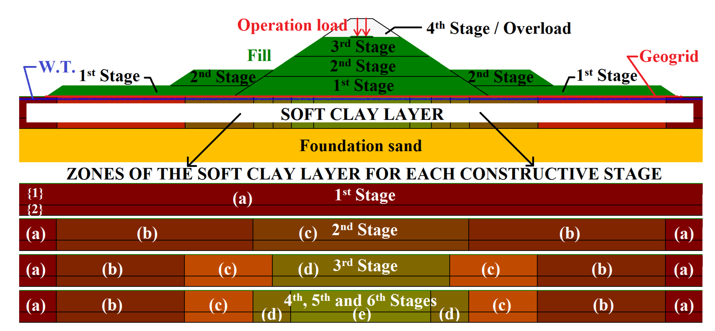
3.1. Model Information

Morgenstern–Price was the analytical method used for the stability analyses, which carries out force and moment equilibrium. At this moment, the slip surfaces were assumed as circular. In addition, the analyses were performed considering the critical moments throughout the construction, in other words, only the moments immediately after executing each stage were analyzed, without time to dissipate the pore water pressure generated in the foundation.

Note that the soft clay layer was divided into vertical zones (Figure 2) for each load stage. For this reason, it was able to take into account the gain of resistance due to the increment of the vertical effective stress ($\Delta {\sigma }_v^{\prime }$), which occurs by loading the surface and dissipating the pore water pressure. Thus, the equation proposed by ref. [45] was used, Equation (6). It also considered the submersion of the embankment and the consolidation percentage at the end of each stage to determine the $\Delta {\sigma }_v^{\prime }$.

$$\Delta S_u=0.22\Delta {\sigma }_v^{\prime }.$$

(6)

Consequently, it obtained the values for each vertical zone of the undrained soft clay foundation, shown in

Table 2. Input parameters of the models.

Parameters	Fill	Sand	Interface	Soft Clay																		Reinf
				${\mathbf{a}}_{\mathbf{1}}$	${\mathbf{a}}_{\mathbf{2}}$	${\mathbf{b}}_{\mathbf{1}}$	${\mathbf{b}}_{\mathbf{2}}$	${\mathbf{c}}_{\mathbf{1}}$	${\mathbf{c}}_{\mathbf{2}}$	${\mathbf{d}}_{\mathbf{1}}$	${\mathbf{d}}_{\mathbf{2}}$	${\mathbf{e}}_{\mathbf{0}-\mathbf{1}}$	${\mathbf{e}}_{\mathbf{0}-\mathbf{2}}$	${\mathbf{b}}_{\mathbf{1}-\mathbf{2}}$	${\mathbf{b}}_{\mathbf{2}-\mathbf{2}}$	${\mathbf{c}}_{\mathbf{1}-\mathbf{2}}$	${\mathbf{c}}_{\mathbf{2}-\mathbf{2}}$	${\mathbf{c}}_{\mathbf{1}-\mathbf{3}}$	${\mathbf{c}}_{\mathbf{2}-\mathbf{3}}$	${\mathbf{e}}_{\mathbf{1}-\mathbf{2}}$	${\mathbf{e}}_{\mathbf{2}-\mathbf{2}}$
$\gamma$ (kN/m${}^3$)	18	17	18	15																		-
$\varphi$’ (${}^{\circ }$)	25.0	35.0	12.5	29.0																		-
c’ (kPa)	25.0	0.0	12.5	-																		-
$S_u$ (kPa)	-			8		16		18		31		45		18		26		28		58		-
$e_0$	-			2.5	1.5	2.5	1.5	2.5	1.5	2.5	1.5	2.5	1.5	2.5	1.5	2.5	1.5	2.5	1.5	2.5	1.5	-
$\lambda$	-			0.456	0.195	0.456	0.195	0.456	0.195	0.456	0.195	0.456	0.195	0.456	0.195	0.456	0.195	0.456	0.195	0.456	0.195	-
$\kappa$	-			0.060	0.025	0.060	0.025	0.060	0.025	0.060	0.025	0.060	0.025	0.060	0.025	0.060	0.025	0.060	0.025	0.060	0.025	-
E (MPa)	15	35	15	2																		-
v	0.3	0.3	0.3	0.45																		-
$OCR$	-			1.2																		-
$K_x$ (m/d)	-			0.001																		-
$J_r$ (MPa)	-			-																		1.5
$T_r$ (kN/m)	-			-																		200

. In addition, this table contains all the parameters used in the model.

Although the soft soil layer was divided into vertical zones, it was also divided into two horizontal zones (1 and 2, see Figure 2 and indexes of the vertical division zones, Table 1). It is worth mentioning that due to the gain of resistance, some zones were duplicated, such as $b_{x-2}$, $c_{x-2}$, $c_{x-3}$, and $e_{x-2}$. In short, the zone configurations for each stage are presented in Table 1.

The constitutive soil models assumed for each material were:

I

For the embankment fill material, foundation sand, and interface element: Drained Elastic-Plastic for the SIGMA/W, and Mohr–Coulomb for the SLOPE/W and SLIDE;

II

For the soft clay material: Soft Clay (Modified Cam-Clay with pore water pressure change) for the SIGMA/W, and Undrained ($\varphi =0^{\circ }$) for the SLOPE/W and SLIDE;

III

For the reinforcement material (geogrid): Structural Beam by considering the Moment of Inertia = 0 m${}^4$ (allowing only tension stress) for the SIGMA/W, and Reinforcement Load by choosing the model developed for geosynthetics for SLOPE/W and SLIDE.

3.2. Statistical Information

Among the related parameters, the following ones were assumed to be random variables: the bulk unit weight ($\gamma$), cohesion (c), undrained shear strength ($S_u$), friction angle ($\varphi$), E-Modulus (E), overconsolidation ratio ($OCR$), initial void ratio ($e_0$), lambda and kappa ($\lambda$ and $\kappa$, referring to the parameters of the Modified Cam-Clay model), hydraulic conductivity (K), and stiffness (J) and tensile strength (T) of the reinforcement. The number of variables to assume as random, for the probabilistic analysis performed by the coupling method, may be limitless. Furthermore, ref. [46] present

Table 3. Distribution and $CoV$s of the parameters assumed as random variables [46].

Parameter	Distribution	$\mathsf{CoV}$ (%)
		min	med	max
Bulk unit weight ($\gamma$)	Normal	2.5	7.5	12.5
Cohesion (c)	Normal	10.0	40.0	70.0
Friction angle ($\varphi$)	Log-Normal	5.0	10.0	15.5
E-Modulus (E)	Normal	2.0	22.0	42.0
Overconsolidation ratio ($OCR$)	Normal	10.0	22.5	35.0
Parameter $\lambda$ of the MCC model	Normal	25.0	27.5	30.0
Parameter $\kappa$ of the MCC model	Normal	25.0	27.5	30.0
Initial void ratio ($e_0$)	Normal	13.0	27.5	42.0
Hydraulic conductivity (K)	Log-Normal	200.0	250.0	300.0
Undrained shear strength ($S_u$)	Log-Normal	20.0	35.0	50.0
Reinforcement stiffness ($J_{geo}$)	Normal	5.0	10.0	15.0
Reinforcement tensile strength ($T_{geo}$)	Normal	5.0	10.0	15.0

, which is based on the analysis of various studies that investigated the distribution and statistical moments (variations) for some geotechnical parameters. The same table and data were assumed for this paper.

The base correlation matrix to be applied for this case is shown in

Table 4. Base correlation matrix for reliability analyses of the models.

Pair	${\mathit{\gamma }}_{\mathit{f}}$	${\mathit{c}}_{\mathit{f}}$	${\mathit{\varphi }}_{\mathit{f}}$	${\mathit{E}}_{\mathit{f}}$	${\mathit{\gamma }}_{\mathit{s}}$	${\mathit{\varphi }}_{\mathit{s}}$	${\mathit{E}}_{\mathit{s}}$	${\mathit{\gamma }}_{\mathit{c}}$	${\mathit{E}}_{\mathit{c}}$	${\mathit{S}}_{\mathit{u},\mathit{a}}$	${\mathit{S}}_{\mathit{u},\mathit{b}}$	${\mathit{S}}_{\mathit{u},\mathit{c}}$	${\mathit{S}}_{\mathit{u},\mathit{d}}$	${\mathit{S}}_{\mathit{u},\mathit{e}}$	$\mathit{OCR}$	${\mathit{\lambda }}_1$	${\mathit{\lambda }}_2$	${\mathit{\kappa }}_1$	${\mathit{\kappa }}_2$	${\mathit{e}}_{0,1}$	${\mathit{e}}_{0,2}$	c${\mathit{K}}_{\mathit{x}}$	${\mathit{J}}_{\mathbf{geo}}$	${\mathit{T}}_{\mathbf{geo}}$
${\gamma }_f$	1	0.5	0.5	0.5	0	0	0	0	0	0	0	0	0	0	0	0	0	0	0	0	0	0	0	0
$c_f$	0.5	1	−0.3	0	0	0	0	0	0	0	0	0	0	0	0	0	0	0	0	0	0	0	0	0
${\varphi }_f$	0.5	-0.3	1	0	0	0	0	0	0	0	0	0	0	0	0	0	0	0	0	0	0	0	0	0
$E_f$	0.5	0	0	1	0	0	0	0	0	0	0	0	0	0	0	0	0	0	0	0	0	0	0	0
${\gamma }_s$	0	0	0	0	1	0.5	0.5	0	0	0	0	0	0	0	0	0	0	0	0	0	0	0	0	0
${\varphi }_s$	0	0	0	0	0.5	1	0	0	0	0	0	0	0	0	0	0	0	0	0	0	0	0	0	0
$E_s$	0	0	0	0	0.5	0	1	0	0	0	0	0	0	0	0	0	0	0	0	0	0	0	0	0
${\gamma }_c$	0	0	0	0	0	0	0	1	0.5	0.5	0.5	0.5	0.5	0.5	0	0	0	0	0	0	0	0	0	0
$E_c$	0	0	0	0	0	0	0	0.5	1	0.5	0.5	0.5	0.5	0.5	0	0	0	0	0	0	0	0	0	0
$S_{u,a}$	0	0	0	0	0	0	0	0.5	0.5	1	0.512	0.354	0.290	0.208	0	0	0	0	0	0	0	0	0	0
$S_{u,b}$	0	0	0	0	0	0	0	0.5	0.5	0.512	1	0.692	0.567	0.407	0	0	0	0	0	0	0	0	0	0
$S_{u,c}$	0	0	0	0	0	0	0	0.5	0.5	0.354	0.692	1	0.820	0.587	0	0	0	0	0	0	0	0	0	0
$S_{u,d}$	0	0	0	0	0	0	0	0.5	0.5	0.290	0.567	0.820	1	0.717	0	0	0	0	0	0	0	0	0	0
$S_{u,e}$	0	0	0	0	0	0	0	0.5	0.5	0.208	0.407	0.587	0.717	1	0	0	0	0	0	0	0	0	0	0
$OCR$	0	0	0	0	0	0	0	0	0	0	0	0	0	0	1	0	0	0	0	0	0	0	0	0
${\lambda }_1$	0	0	0	0	0	0	0	0	0	0	0	0	0	0	0	1	0.368	0.7	0	0	0	0	0	0
${\lambda }_2$	0	0	0	0	0	0	0	0	0	0	0	0	0	0	0	0.368	1	0	0.7	0	0	0	0	0
${\kappa }_1$	0	0	0	0	0	0	0	0	0	0	0	0	0	0	0	0.7	0	1	0	0	0	0	0	0
${\kappa }_2$	0	0	0	0	0	0	0	0	0	0	0	0	0	0	0	0	0.7	0	1	0	0	0	0	0
$e_{0,1}$	0	0	0	0	0	0	0	0	0	0	0	0	0	0	0	0	0	0	0	1	0.368	0.5	0	0
$e_{0,2}$	0	0	0	0	0	0	0	0	0	0	0	0	0	0	0	0	0	0	0	0.368	1	0	0	0
$K_x$	0	0	0	0	0	0	0	0	0	0	0	0	0	0	0	0	0	0	0	0.5	0	1	0	0
$J_{geo}$	0	0	0	0	0	0	0	0	0	0	0	0	0	0	0	0	0	0	0	0	0	0	1	0.5
$T_{geo}$	0	0	0	0	0	0	0	0	0	0	0	0	0	0	0	0	0	0	0	0	0	0	0.5	1

. It was built by taking into account the applications and studies developed by refs. [16,17,47]. By joining the highlighted terms of the base correlation matrix, it built the correlation matrix used in the stability analysis by the LEM, while the entire base correlation matrix was assumed for the postconstruction settlement analysis by the FEM.

The horizontal and vertical correlations among the parameters for each zone, such as $S_u$, $\lambda$, and $e_0$, were assumed according to the exponential model (Equation (7)) used by ref. [16], which was adopted to describe the spatial variation.

$${\rho }_{ij}=exp\left(-\frac{\left|Position\left(i\right)-Position\left(j\right)\right|}{d}\right).$$

(7)

Therefore, it was able to evaluate the probability of failure for each constructive stage by considering the unreinforced embankment, as well as the same one by assuming the introduction of a basal reinforcement with a geogrid. The coupling between StRAnD (reliability academic software) and the SLOPE/W, SIGMA/W or SLIDE (LEM and FEM commercial software, belonging to the GeoStudio and RocScience pack) was able to carry out the reliability analyses.

3.3. Limit State (LS) Function

3.3.1. Slope Stability

In this paper, the LS function was assumed to be $g\left(\mathit{X}\right)=R\left(\mathit{X}\right)-A\left(\mathit{X}\right)$. The $R\left(\mathit{X}\right)$ and $A\left(\mathit{X}\right)$ are the sum function of resisting and activating, respectively, of forces and/or moments (depending on the LEM chosen) along the critical slip surface.

Usually, the LS function is adapted to be $g\left(\mathit{X}\right)=FS\left(\mathit{X}\right)-1$. The $FS$ value results from the ratio of $R\left(\mathit{X}\right)$ and $A\left(\mathit{X}\right)$, which may make this function highly nonlinear. The fact is the greater the nonlinearity of the performance function, the more the advantages of the transformation method use are lost (the relatively low computational cost). Sometimes, this can lead the analysis to a condition of nonconvergence or to wrong results. Therefore, for the analyses in this paper, the first defined LS function was used.

3.3.2. Postconstruction Settlement

To demonstrate the possibilities that the coupling method can evaluate, a postconstructional settlement analysis was also assumed for a time of 180 days after constructing the structure. For this reason, the LS function was assumed to be $g\left(\mathit{X}\right)=\Delta \delta \left(\mathit{X}\right)-\Delta {\delta }_{max}$, for this analysis. The $\Delta \delta \left(\mathit{X}\right)$ is the difference of the maximum vertical displacement between the last constructive stage and 180 days after this stage. The $\Delta {\delta }_{max}$ represents the maximum acceptable displacement as this time goes by.

4. Results

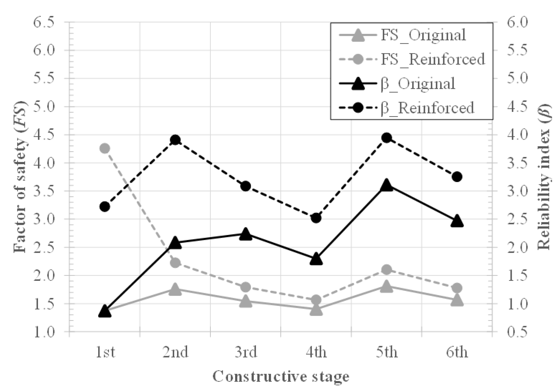
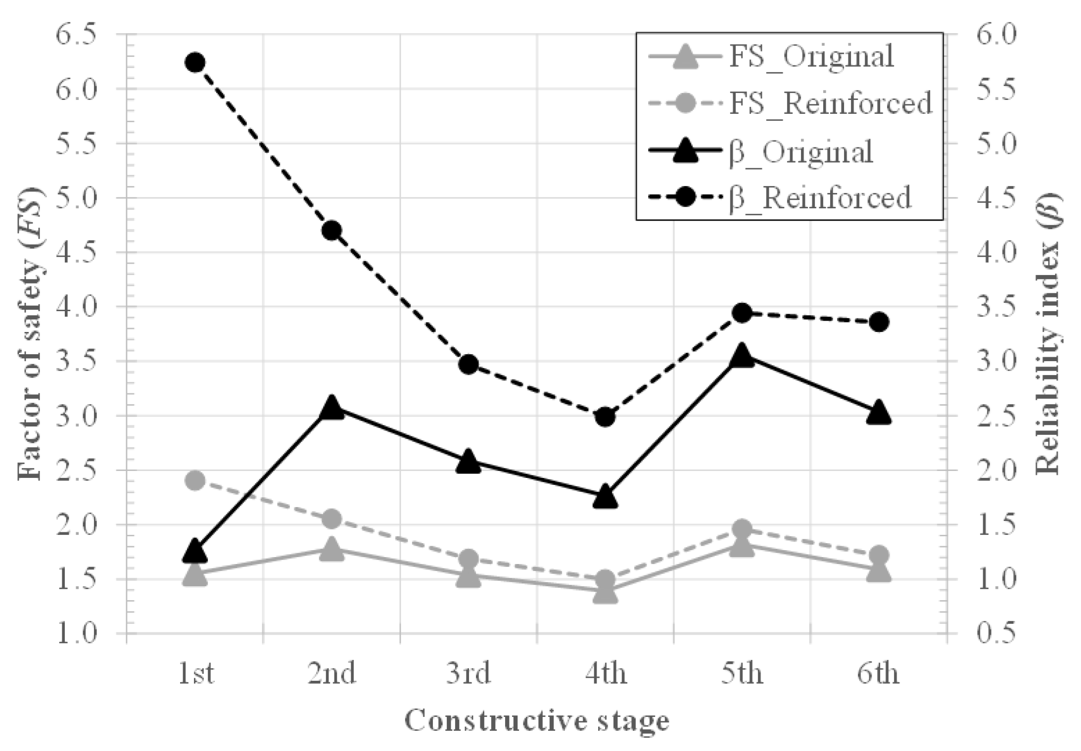
4.1. Deterministic and Probabilistic Stability Analysis

First, the deterministic stability analyses of the original and reinforced configuration were carried out by using the commercial programs. Next, these models were probabilistically analyzed by the coupling method adapted for this purpose and assuming the medium values of $CoV$. Figure 3 and Figure 4 show the results obtained for both analyses, first using the coupling for SLOPE/W and then the other one for SLIDE. The deterministic results ($FS$) are represented by the principal vertical axis, while the second represents the probabilistic results ($\beta$).

Note that the minimum $FS$ obtained for the models was around 1.37 for SLOPE/W and 1.39 for SLIDE, both of the original configurations. According to ref. [44], the safety requirement for this structure was assumed to reach the minimum $FS$ equal to 1.30 and 1.50, for the construction phases and for the operational one (6th Stage), respectively. Consequently, the $FS$ obtained by both software and for all stages was satisfactory.

However, the minimum value of $\beta$ obtained was around 0.87 at the first stage of the original configuration. This is a low value for $\beta$, which represents a $Pf$ higher than 19%, and therefore, it is considered a dangerous condition, according to ref. [48].

By comparing the gain of $FS$ due to the reinforcement introduction, it shows a greater improvement for the 1st and 2nd Stages. For the next stages, the improvement becomes almost constant. These behaviors are common to the results of both programs and persist in the reliability analysis. They are also able to conclude that the behavior of the values of $\beta$ with stages is similar to the behavior of the $FS$.

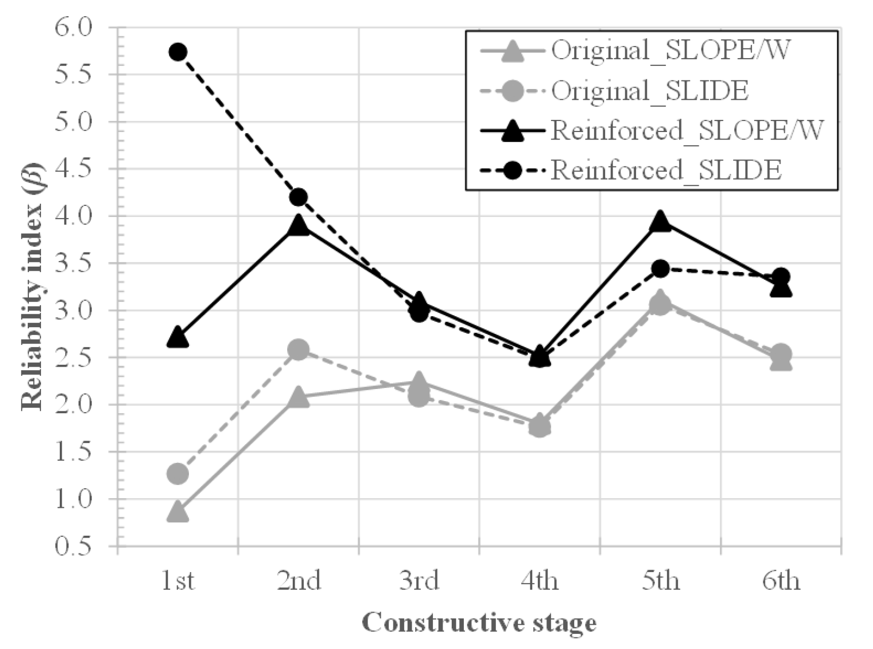
4.2. Comparison of the Probabilistic Performance of Both Couplings

A comparison of the values of $\beta$ resulting from both couplings is presented in Figure 5. Note that the reliability indexes from the same stage and configuration are closer to each other, despite the fact that they were carried out by coupling for different commercial software.

Only the first stage of the reinforced configuration showed a significant degree of the unconformity between program usage. However, it may be associated with the following aspects:

• About how programs assumed the behavior of the reinforcement in the simulation: Precisely, in this study, SLOPE/W took the mobilized reinforcement strength to reduce the activating forces/moments. By contrast, SLIDE assumed the reinforcement strength to increase the resisting forces/moments. Since reinforcement is overdesigned for the first stage (i.e., reinforcement is supposed to work for the last stage, operation), the program assumption presents significant effects for this stage. Indeed, reinforcement at the first stage would most likely resist most of the actions due to the beginning of the surface loading. Consequently, the $FS$ and $\beta$ are likely to assume high initial values because the reinforcement is supposed to help the foundation soil up to after the sixth stage when the excess of pore water pressure dissipates;
• Each software assumed the searching surface method: Simulations with SLOPE were carried out by adopting the entry and exit search method. At the same time, SLIDE evaluated the stability by running the auto search surface algorithm. Then, discrepancies are expected regarding each simulation’s defined critical slip surface. The critical slip surface may also vary according to configurations assumed for the searching method (e.g., iteration number, node numbers);
• Finally, it is essential to note that critical surfaces do not have to be coincident when comparing the deterministic critical slip surface and the probabilistic one [13,14,15]. The likely change of critical slip surface location at each simulation may also affect the results, mainly for the first stages, associated with significant geometry changes because of the equilibrium berms.

Therefore, it can be concluded that both couplings presented similar and satisfactory results.

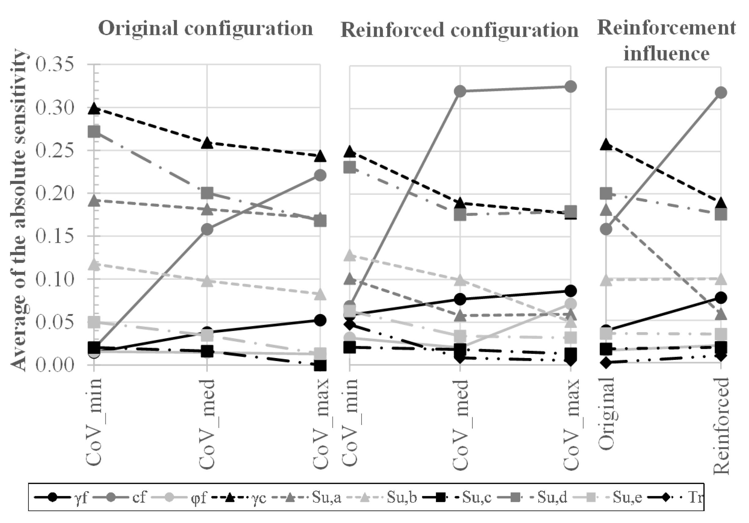
4.3. Influence of the Uncertainty Level of the Stability

By using the coupling to SLOPE/W, the analysis of the model was carried out by assuming different levels of $CoV$ (uncertainty). These levels were assumed to be minimum, medium, and maximum, as shown in Table 3. Figure 6 shows the values of $\beta$ obtained for each stage and configuration.

As expected, both configurations show a tendency to decrease the value of $\beta$ when the uncertainty level ($CoV$) is increased, and this trend is quite significant. For example, this made safety fall from a high-performance level (according to ref. [48]), in the reinforced configuration ($\beta >5.0$), to a below-average, poor, and even unsatisfactory level ($\beta \approx$ 2.5, 2.0, and 1.5, respectively). Likewise, for the original configuration, it falls from a poor performance level ($\beta \approx 2.0$), in the worst safety index stage (1^st), to a level worse than dangerous ($\beta <1.0$).

Although this influence was obtained in an exaggerated way, it reflects how much the uncertainty level of the parameters can change the safety condition in the reliability analysis. However, it is extremely plausible to assume uncertainty levels, such as those presented in this paper because the less that is known about the soil behavior and its parameter values, the higher level of uncertainty needs to be adopted. In the same way, a low level of uncertainty may be adopted for a situation where the soil behavior and its parameter values are known, which leads to more reliable results and realistic behaviors.

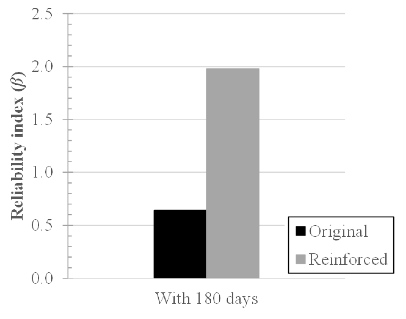
4.4. Probabilistic Performance of the Postconstruction Settlement

In order to demonstrate another range of possibilities that the coupling method is able to provide, it was probabilistically analyzed that the value of $\beta$ regarding the postconstruction settlement does not exceed a predetermined vertical displacement value. Accordingly, it used the coupling method for the SIGMA/W software.

First, the deterministic vertical displacement was obtained for 180 days from the sixth stage. The original configuration presented a maximum vertical displacement around 48 mm, while the reinforced one assumed around 32 mm. Thus, a vertical displacement limit of 60 mm was adopted. This limit was introduced into the LS function, as mentioned. Figure 7 shows the value of $\beta$ for this condition, i.e., the reliability or probability that this vertical displacement is exceeded, which starts from a value of $\beta$ close to 0.64 ($Pf\approx$ 26.0%) in the original configuration to a value of $\beta$ approximately 1.98 ($Pf\approx$ 2.4%) in the reinforced configuration.

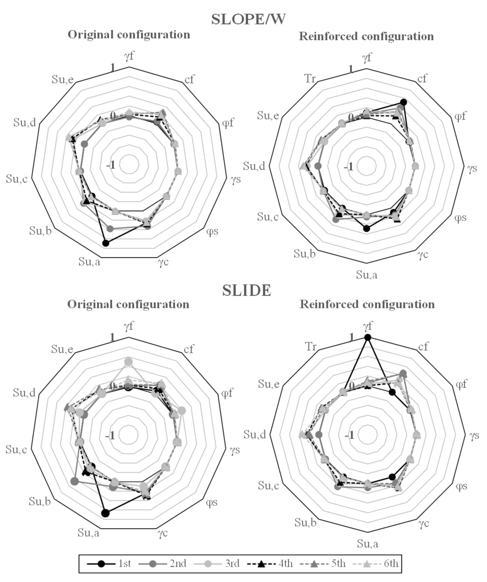
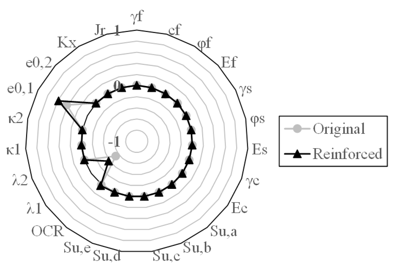
4.5. Sensitivity of the Parameters

As described before, the coupling method is able to acquire information about the sensitivity of the random variables. Figure 8 shows the sensitivity results for each parameter assumed as a random variable in the stability analysis, for both couplings of SLOPE/W and SLIDE. In the same way, Figure 9 presents this for the random variables of the analysis of the postconstruction settlement.

For both SLOPE/W and SLIDE, it can be seen that there is a strong influence of the undrained shear strength and the zone with greater influence changes for each stage, which may assume over one for each stage. This happens according to the position of the probabilistic critical slip surface, which makes the zones that are crossed by it into zones with a higher influence. It is also worth mentioning that the bulk unit weight of the soft clay showed a significant influence on both configurations and couplings. On the other hand, the parameters that did not present a significant sensitivity level could be adopted as deterministic parameters to make the computational process faster.

Concerning the sensitivity results of the postconstruction settlement analysis, they showed a dominant influence of the initial void ratio and $\lambda$ of the Modified Cam-Clay (MCC) model (related to the compressibility index) from the superficial soft clay layer. The other parameters showed no influence (in this case) and could be adopted as deterministic parameters.

In addition to the sensitivity analysis, the influence of the uncertainty level and the reinforcement introducing the sensitivity of the parameters were also analyzed. Figure 10 shows the result in terms of the average of the absolute sensitivity values for each stage.

The influence of uncertainty in the analysis shows that the great sensitivity parameters can change according to the uncertainty level. Moreover, some random variables may begin closer to a null sensitivity (for the minimum $CoV$) and become one of the most sensitive parameters (for the maximum $CoV$), such as the cohesion of the fill material.

By comparison, the sensitivity of $S_u$ decreases when the reinforced configuration is analyzed. In addition, cohesion sensitivity becomes greater. In other words, the cohesion influences the interface parameters between the soil and the reinforcement, such as the adhesion force. Both coupling analyses have presented this behavior (Figure 8).

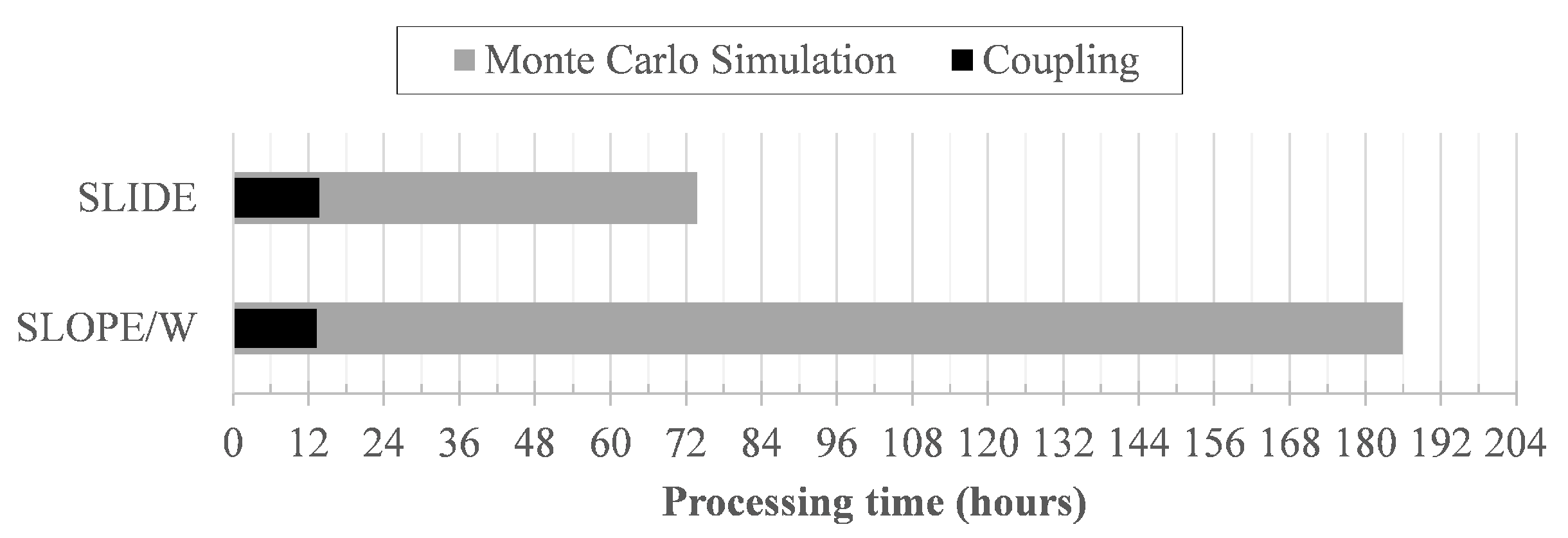
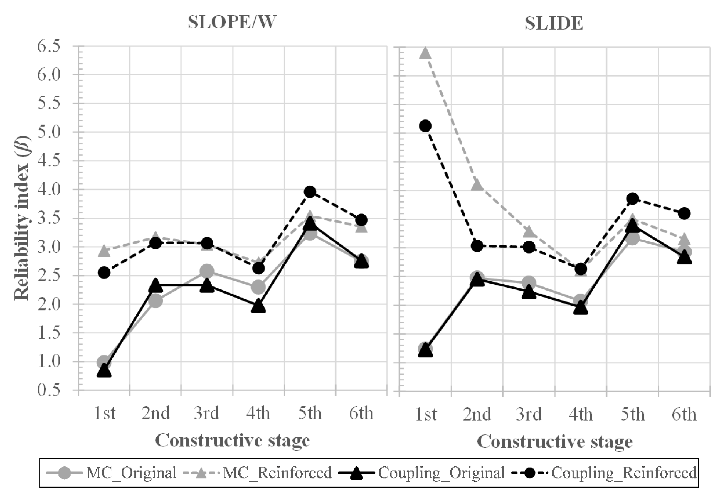
4.6. Validation of the Coupling Method

Finally, in order to validate the coupling method and demonstrate the greater advantage of this usage, the case study was carried out in the commercial programs to evaluate the values of $\beta$ for each stage using the Crude MC simulation method. However, the parameters were adopted to be independent because the commercial programs were not able to assume some of the proposed correlations. In other words, it was assumed that there were no correlations between the variable pairs. Then, the coupling method was carried out again for both configurations and programs.

It is important to note that this study used previous software versions (i.e., SLOPE/W 2016 and SLIDE v.6.0). Nowadays, the programs have shown significant evolution regarding probabilistic analysis since those versions (e.g., being able to handle a wider range of correlation options, work with other probabilistic methods, and consider new parameters as random variables).

According to ref. [34], the number of required samples to develop the Crude MC simulation method can be estimated by ${10}^{p+2}$. The term p is related to the magnitude of the probability of failure (${10}^{-p}$).

Note that the analyses with medium $CoV$s resulted in the value of $\beta$ around 2.3 and 3.0 for the original and reinforced configuration, respectively. This means that the probability of failure is in the order of ${10}^{-2}$ and ${10}^{-3}$, respectively. As a result, at least ${10}^4$ and ${10}^5$ samples (evaluations) are needed for a good estimation. Then, 10,000 and 100,000 samples were adopted for SLOPE/W and SLIDE, respectively, and for both configurations. It is worth pointing out that due to the high computational cost required for commercial programs to carry out a high number of samples, higher values of $\beta$ were not able to present a good prediction.

The values of $\beta$ obtained using the MC simulation and coupling method are compared and presented in Figure 11. It can be concluded that the values of $\beta$ were very similar for both commercial programs and particularly for the original configuration. As expected, higher variances are associated with the reinforced configuration and for high values of $\beta$ because of the number of samples that were adopted and fixed for each program. Another point is that the SLIDE MC simulation provides closer values to the coupling ones because it was carried out with a higher number of samples: 10 times higher.

Besides the prediction validation, the required evaluation time for the MC simulation in the commercial software and for the FORM in the coupling method was also evaluated to carry out a complete analysis of all six stages of one configuration (original). The results were compared and presented in Figure 12. As a result, the coupling method was much faster than the MC simulation method in commercial software. On the one hand, for both couplings, the required time was around 13 h and 30 min (around half a day). On the other hand, the MC simulation required around 186 (almost 8 days) and 74 h (around 3 days) for SLOPE/W (10,000 samples) and SLIDE (100,000 samples), respectively. In particular, there were some stages of the coupling method that required only 4–5 min to be carried out, while other ones needed almost 4 h to be evaluated. Therefore, this evaluation time could be shorter and also longer, depending on the nonlinearity of the LS function, which influences the convergence time.

5. Conclusions

A coupling method was presented in order to demonstrate a practical method to introduce reliability analysis into LEM and FEM programmed by common commercial software. To illustrate this, a stage-constructed embankment was analyzed, and two configurations were assumed; first, an original configuration proposed by ref. [44] and another one, similar to the first, only by adding a basal geosynthetic reinforcement (geogrid). Thus, this paper was able to provide the following conclusions supported by the following results:

• The coupling method can be used with different commercial programs, widely used in the practical field. In this paper, for example, the reliability analyses were obtained from the application to two well-known commercial programs, GeoStudio (SLOPE/W and SIGMA/W) and RocScience (SLIDE);
• The coupling method can carry an analysis by using LEM and FEM. Indeed, it may be also applied to other methods, such as discrete elements and material point methods;
• Comparing the results obtained via the coupling method and the crude MC simulation, the coupling approach presents great precision to approximate the value of $\beta$ using the FORM, as shown by Figure 11. Besides the precision, it is also able to perform a probabilistic analysis with a much lower computational cost; about 7.3% (13.8 times faster) and 18.2% (5.5 times faster) of the total required time by GeoStudio and RocScience, respectively, to process the analysis;
• Besides analyzing the probabilistic stability of the embankment, the coupling method can also carry out probabilistic analysis over several other aspects as these may be described by an LS function. For example, besides the stability condition, a probabilistic analysis was also carried out concerning the postconstruction settlement for the case study;
• By understanding the coupling method, the value of $\beta$ obtained from this cannot be associated with a specific slip surface. As pointed out by the literature, the probabilistic critical slip surface does not coincide with the deterministic one because each evaluation of the model with a different $\mathit{X}$ may present different results for the critical slip surface position. Then, it is right to say that the value of $\beta$ obtained by the coupling method refers to the stability or to another aspect associated with the LS function of the entire system, not to a specific slip surface, even though it is the probabilistic one;
• Most probabilistic studies and practice analysis of embankments, even having been constructed by stages and built on soft ground, usually carried out analyses just for the last stage. However, the value of $\beta$ may vary significantly with stages and time, such as those presented by this paper;
• Considering only the deterministic $FS$ obtained for the models, it can be concluded that the original structure presented a satisfactory safety level (according to the design requirements adopted by the reference). However, the reliability analyses showed another reality where the structure was considered unsatisfactory, according to [48]. As a result, to acquire a good estimation of the safety level and to obtain reliable results during the design conception, both indexes ($FS$ and $\beta$) need to be tested;
• The probabilistic safety level is strongly influenced by the uncertainty level assumed for the system. This influence may take the structure of a high level of performance to an unsatisfactory level even worse than it. Therefore, it is strongly recommended that $CoV$ be taken according to the tests performed in situ and only if these tests present a satisfactory number of samples, particularly for the most sensitive parameters. The less known about the structure and the parameters involved, the higher the level of uncertainty ($CoV$ values) is to be adopted;
• The coupling method analyzes the whole process and the convergence history. These data are helpful to identify potential problems or to add other analyses throughout the process, which makes the method more reliable.

In conclusion, the coupling method presents significant advantages, such as great precision to approximate the reliability index, using FORM, with a much lower computational cost. It can also evaluate different aspects of the system (geotechnical structure) in a probabilistic way. Finally, the biggest advantage of this method is the fact that is able to couple to common geotechnical programs, as was shown in this paper, which are widely used in the practical field. Therefore, this can be easily applied when developing geotechnical structure designs.

References

1. Cornell, C.A. First order uncertainty analysis of soils deformations and stability. In Proceedings of the 1st International Conference on Application of Statistics and Probability in Soil and Structural Engineering, Hong Kong, China, 13–16 September 1971; pp. 129–144. [Google Scholar]
2. Tang, W.; Yucemen, M.; Ang, A. Probability-based short term design of slopes. Can. Geotech. J. 1976, 13, 201–215. [Google Scholar] [CrossRef]
3. McGuffey, V.; Grivas, D.; Iori, J.; Kyfor, Z. Conventional and Probabilistic Embankment Design. J. Geotech. Eng. Div. 1982, 108, 1246–1254. [Google Scholar] [CrossRef]
4. Oka, Y.; Wu, T.H. System Reliability of Slope Stability. J. Geotech. Eng. 1990, 116, 1185–1189. [Google Scholar] [CrossRef]
5. Chowdhury, R.N.; Xu, D.W. Rational Polynomial Technique in Slope Reliability Analysis. J. Geotech. Eng. 1993, 119, 1910–1928. [Google Scholar] [CrossRef]
6. Alonso, E.E. Risk analysis of slopes and its application to slopes in Canadian sensitive clays. Géotechnique 1976, 26, 453–472. [Google Scholar] [CrossRef]
7. Harr, M.E. Mechanics of Participate Media: A Probabilistic Approach; McGraw-Hill International: New York, NY, USA, 1977; p. 543. [Google Scholar]
8. Vanmarcke, E.H. Reliability of earth slopes. J. Geotech. Eng. Div. 1977, 103, 1247–1265. [Google Scholar] [CrossRef]
9. Chowdhury, R.N.; A-Grivas, D. Probabilistic Model of Progressive Failure of Slopes. J. Geotech. Eng. Div. 1982, 108, 803–819. [Google Scholar] [CrossRef]
10. Bergado, D.; Miura, N.; Chang, J.; Danzuka, M. Reliability assessment of test embankments on soft Bangkok clay by variance reduction and nearest-neighbor methods. Comput. Geotech. 1987, 4, 171–194. [Google Scholar] [CrossRef]
11. Christian, J.T.; Ladd, C.C.; Baecher, G.B. Reliability Applied to Slope Stability Analysis. J. Geotech. Eng. 1994, 120, 2180–2207. [Google Scholar] [CrossRef]
12. Bergado, D.T.; Patron, B.C.; Youyongwatana, W.; Chai, J.C.; Yudhbir. Reliability-based analysis of embankment on soft Bangkok clay. Struct. Saf. 1994, 13, 247–266. [Google Scholar] [CrossRef]
13. Chowdhury, R.N.; Tang, W.H. Comparison of risk models for slopes. In Proceedings of the 5th International Conference on Application of Statistics and Probability in Soil and Structural Engineering; University of British Columbia: Vancouver, BC, Canada, 1987; pp. 863–869. [Google Scholar]
14. Li, K.S.; Lumb, P. Probabilistic design of slopes. Can. Geotech. J. 1987, 24, 520–535. [Google Scholar] [CrossRef]
15. Hassan, A.M.; Wolff, T.F. Search Algorithm for Minimum Reliability Index of Earth Slopes. J. Geotech. Geoenviron. Eng. 1999, 125, 301–308. [Google Scholar] [CrossRef]
16. Low, B.; Tang, W.H. Probabilistic slope analysis using Janbu’s generalized procedure of slices. Comput. Geotech. 1997, 21, 121–142. [Google Scholar] [CrossRef]
17. Low, B.; Tang, W.H. Reliability analysis of reinforced embankments on soft ground. Can. Geotech. J. 1997, 34, 672–685. [Google Scholar] [CrossRef]
18. Low, B.K.; Gilbert, R.B.; Wright, S.G. Slope Reliability Analysis Using Generalized Method of Slices. J. Geotech. Geoenviron. Eng. 1998, 124, 350–362. [Google Scholar] [CrossRef]
19. El-Ramly, H.; Morgenstern, N.; Cruden, D. Probabilistic slope stability analysis for practice. Can. Geotech. J. 2002, 39, 665–683. [Google Scholar] [CrossRef]
20. Bhattacharya, G.; Jana, D.; Ojha, S.; Chakraborty, S. Direct search for minimum reliability index of earth slopes. Comput. Geotech. 2003, 30, 455–462. [Google Scholar] [CrossRef]
21. Wang, Y.; Cao, Z.; Au, S.K. Efficient Monte Carlo Simulation of parameter sensitivity in probabilistic slope stability analysis. Comput. Geotech. 2010, 37, 1015–1022. [Google Scholar] [CrossRef]
22. Zhang, L.; Zhang, J.; Zhang, L.; Tang, W. Back analysis of slope failure with Markov chain Monte Carlo simulation. Comput. Geotech. 2010, 37, 905–912. [Google Scholar] [CrossRef]
23. Kang, F.; Han, S.; Salgado, R.; Li, J. System probabilistic stability analysis of soil slopes using Gaussian process regression with Latin hypercube sampling. Comput. Geotech. 2015, 63, 13–25. [Google Scholar] [CrossRef]
24. Marandi, S.; Anvar, M.; Bahrami, M. Uncertainty analysis of safety factor of embankment built on stone column improved soft soil using fuzzy logic α-cut technique. Comput. Geotech. 2016, 75, 135–144. [Google Scholar] [CrossRef]
25. Ferreira, F.B.; Topa Gomes, A.; Vieira, C.S.; Lopes, M.L. Reliability analysis of geosynthetic-reinforced steep slopes. Geosynth. Int. 2016, 23, 301–315. [Google Scholar] [CrossRef]
26. Xia, Y.; Mahmoodian, M.; Li, C.Q.; Zhou, A. Stochastic Method for Predicting Risk of Slope Failure Subjected to Unsaturated Infiltration Flow. Int. J. Geomech. 2017, 17, 04017037. [Google Scholar] [CrossRef]
27. Wang, F.; Li, H.; Zhang, Q.L. Response-Surface-Based Embankment Reliability under Incomplete Probability Information. Int. J. Geomech. 2017, 17, 06017021. [Google Scholar] [CrossRef]
28. Javankhoshdel, S.; Bathurst, R.J. Deterministic and probabilistic failure analysis of simple geosynthetic reinforced soil slopes. Geosynth. Int. 2017, 24, 14–29. [Google Scholar] [CrossRef]
29. Mouyeaux, A.; Carvajal, C.; Bressolette, P.; Peyras, L.; Breul, P.; Bacconnet, C. Probabilistic stability analysis of an earth dam by Stochastic Finite Element Method based on field data. Comput. Geotech. 2018, 101, 34–47. [Google Scholar] [CrossRef]
30. Santos, M.G.C.; Silva, J.L.; Beck, A.T. Reliability-based design optimization of geosynthetic-reinforced soil walls. Geosynth. Int. 2018, 25, 442–455. [Google Scholar] [CrossRef]
31. Ji, J.; Liao, H.; Low, B. Modeling 2-D spatial variation in slope reliability analysis using interpolated autocorrelations. Comput. Geotech. 2012, 40, 135–146. [Google Scholar] [CrossRef]
32. Low, B. FORM, SORM, and spatial modeling in geotechnical engineering. Struct. Saf. 2014, 49, 56–64. [Google Scholar] [CrossRef]
33. Jia, J.; Wang, S.; Zheng, C.; Chen, Z.; Wang, Y. FOSM-based shear reliability analysis of CSGR dams using strength theory. Comput. Geotech. 2018, 97, 52–61. [Google Scholar] [CrossRef]
34. Melchers, R.E.; Beck, A.T. Structural Reliability Analysis and Prediction, 3th ed.; John Wiley & Sons, Ltd.: Hoboken, NJ, USA, 2017; p. 506. [Google Scholar] [CrossRef]
35. Hasofer, A.M.; Lind, N.C. Exact and Invariant Second-Moment Code Format. J. Eng. Mech. Div. 1974, 100, 111–121. [Google Scholar] [CrossRef]
36. Rackwitz, R.; Flessler, B. Structural reliability under combined random load sequences. Comput. Struct. 1978, 9, 489–494. [Google Scholar] [CrossRef]
37. Ellingwood, B.R. Reliability-based condition assessment and LRFD for existing structures. Struct. Saf. 1996, 18, 67–80. [Google Scholar] [CrossRef]
38. Nataf, A. Détermination des distributions de probabilités dont les marges sont données. Comptes Rendus L’AcadéMie Des Sci. 1962, 225, 42–43. [Google Scholar]
39. Lebrun, R.; Dutfoy, A. A generalization of the Nataf transformation to distributions with elliptical copula. Probabilistic Eng. Mech. 2009, 24, 172–178. [Google Scholar] [CrossRef]
40. Lebrun, R.; Dutfoy, A. An innovating analysis of the Nataf transformation from the copula viewpoint. Probabilistic Eng. Mech. 2009, 24, 312–320. [Google Scholar] [CrossRef]
41. Lebrun, R.; Dutfoy, A. Do Rosenblatt and Nataf isoprobabilistic transformations really differ? Probabilistic Eng. Mech. 2009, 24, 577–584. [Google Scholar] [CrossRef]
42. Baecher, G.; Christian, J. Reliability and Statistics in Geotechnical Engineering; John Wiley & Sons Ltd.: London, UK, 2003; p. 618. [Google Scholar]
43. Beck, A.; Verzenhassi, C. Risk optimization of a steel frame communications tower subject to tornado winds. Lat. Am. J. Solids Struct. 2008, 5, 187–203. [Google Scholar]
44. Nascimento, C.M.C. Avaliação de Alternativas de Processos Construtivos de Ferrovias Sobre Solos Moles. Specialization Thesis, Military Institute of Engineering, Rio de Janeiro, RJ, Brazil, 2008. (In Portuguese). [Google Scholar]
45. Mesri, G. New design procedure for stability of soft clays. J. Geotech. Geoenvironmental Eng. 1975, 101, 409–412. [Google Scholar] [CrossRef]
46. Belo, J.L.P.; Silva, J.L. Reliability Analysis of a Controlled Stage-Constructed and Reinforced Embankment on Soft Ground Using 2D and 3D Models. Front. Built Environ. 2020, 5, 150. [Google Scholar] [CrossRef] [Green Version]
47. Azzouz, A.S.; Krizek, R.J.; Corotis, R.B. Regression Analysis of Soil Compressibility. Soils Found. 1976, 16, 19–29. [Google Scholar] [CrossRef] [Green Version]
48. USACE. Engineering and Design: Introduction to Probability and Reliability Methods for Use in Geotechnical Engineering; Technical Letter CECW-EG – ETL 1110-2-547; U.S. Army Corps of Engineers: Washington, DC, USA, 1997. [Google Scholar]
Figure 1. Flowchart of the coupling method performance.
Sustainability 14 02224 g001
Figure 2. Embankment geometry and zone division for soft clay layer.
Sustainability 14 02224 g002
Figure 3. Deterministic ( F S ) and probabilistic ( β ) results for the stability analysis of both situations (original and reinforced) throughout the stages—coupling with SLOPE/W.
Sustainability 14 02224 g003
Figure 4. Deterministic ( F S ) and probabilistic ( β ) results for the stability analysis of both situations (original and reinforced) throughout the stages—coupling with SLIDE.
Sustainability 14 02224 g004
Figure 5. Comparison of the reliability indexes for the stability analyses between both situations and by coupling to SLOPE/W and SLIDE, with stages.
Sustainability 14 02224 g005
Figure 6. Reliability indexes for the embankment stability with stages by assuming different uncertainty levels, conducted for both configurations.
Sustainability 14 02224 g006
Figure 7. Reliability indexes for the performance of the postconstruction settlement on the 180th day for both configurations.
Sustainability 14 02224 g007
Figure 8. Sensitivity analysis for the stability analysis for both configurations and couplings.
Sustainability 14 02224 g008
Figure 9. Sensitivity analysis for the performance of the postconstruction settlement for both configurations.
Sustainability 14 02224 g009
Figure 10. The influence of the uncertainty level and of the reinforcement (with medium CoV) in the sensitivity of the parameters.
Sustainability 14 02224 g010
Figure 11. Comparison of the reliability indexes for both configurations run by MC simulation (within SLOPE/W) and by the coupling software—no correlation applied.
Sustainability 14 02224 g011
Figure 12. Comparison of the processing time required by MC simulation (using the SLOPE/W and the SLIDE) and by the coupling software.
Sustainability 14 02224 g012