1. Introduction
The presence of suspended matter in surface water makes the water turbid, reduces the water transparency, affects the respiration and metabolism of aquatic organisms (even causing fish suffocation and death) and might cause channel obstruction. Suspended matter concentration is one of the important indices for surface water quality monitoring [
1]. Suspended matter in water absorbs or scatters light entering the water; thus, it affects the optical properties of the water [
2]. Water color remote sensing technology provides an effective way to estimate the concentration of large-scale suspended matter. The remote sensing inversion of water quality parameters provides efficient, fast and high-precision monitoring tools for water quality monitoring, making the environmental governance of surface water more reliable [
3]. It is time-consuming to use traditional water quality monitoring methods and they have failed to meet the needs of large-scale water quality monitoring. Considering that various water resource problems are emerging, there is an urgent need for more efficient and accurate assessment tools to protect and maintain the quantity and quality of water resources [
4]. More and more researchers have focused on using remote sensing technology to solve the problem of water quality monitoring. They have tried to conduct inversion with different types of remote sensing data, optimized inversion algorithms and built new inversion models in order to obtain more accurate inversion results [
5,
6]. However, the inversion results are often limited in accuracy because of the optical complexity of the water environment, the interaction among the water quality parameters, remote sensing image processing and so on; thus, the concentration and distribution of water quality parameters cannot be obtained timely and efficiently. For the existing problems mentioned above, it is necessary to propose more efficient and accurate inversion methods for water quality parameters.
Common remote sensing data used in water quality parameter inversion include MODIS [
7,
8,
9], Landsat TM [
10,
11], Landsat 8 OLI [
12], Sentinel-2 [
13,
14,
15], GF-1 WFV [
16,
17,
18] and hyperspectral images [
19,
20,
21]. These remote sensing data are mostly used for remote sensing monitoring and the evaluation of water quality and for the development of a remote sensing inversion model of water quality parameters. Even though increasingly abundant remote sensing image data are used in water quality parameter inversion, data from different satellites and sensors have their own characteristics and thus are used to invert different water quality parameters. Previous comparison studies have indicated that various remote sensing image data have divergent performances in different areas and different water quality parameter inversions. Gaofen-2 (GF-2) is the highest-resolution civilian land observation satellite in China. Its spatial resolution of satellites under the point could reach 0.8 m, which is significantly better than both Landsat 8 OLI and Environment-1 CCD data [
22]. The number of data bands of GF-2 is smaller than that of Landsat 8 OLI data. However, it contains four bands just within the main spectral range for the inversion of suspended matter concentration. Clearly, GF-2 satellite data are fully suitable to build the remote sensing inversion models for suspended matter and to be applied in inland water quality monitoring.
At present, there are many remote sensing algorithms to retrieve water quality parameter concentration [
23,
24,
25]. In the process of developing algorithms, the functional form of the algorithm is determined, the function of the parameters is derived from a set of input and output pairs and these data have an impact on the scope of the trained data set and the model performance; besides, the non-linearity of water quality parameters has certain restrictions on the algorithm. These issues make the remote sensing inversion of water quality parameters more challenging. Statistical regression [
26,
27], neural networks [
28,
29,
30,
31] and other methods have been used to build water quality parameter inversion models. However, with the increasing accuracy requirements for water quality parameter inversion, more and more studies have been conducted to improve the original inversion model by optimizing and building new models to improve the inversion results of water quality parameters [
32,
33,
34]. Some researchers have developed models based on semi-analytical algorithms to utilize multispectral and hyperspectral remote sensing to draw algal concentrations in inland waters. An optical model to determine parameter concentrations has been developed based on the optical properties of some substances contained in the algae attenuation and backscattering of other optically active components in turbid inland waters [
35]. For water quality parameter inversion, multiple linear stepwise regression is a common linear method. However, due to the complexity of surface influences, the relationship between surface water quality parameters and high-resolution data does not strictly follow linear statistical law. In recent decades, the application of some non-linear methods, such as neural networks [
36], random forest [
37,
38], fuzzy recognition [
39,
40], principal component regression [
41,
42], least squares regression [
43,
44] and quadratic polynomial stepwise regression, have advanced the research on water quality parameter inversion. Based on this, many researchers have further developed and applied these methods to propose some new methods, including support vector machines for particle swarm optimization (PSO) [
45,
46] and modified gray correlations [
47]. Since ordinary neural networks tend to fall into local minimal values during the training process, a new method for optimizing neural networks has been proposed. Among the improved back-propagation neural network (BPNN) algorithms, commonly used ones include the particle swarm optimization algorithm and the genetic algorithm. The genetic algorithm cannot solve the problem of high-dimension optimization when the population size is from 30 to 50 and it is unable to obtain better results at a large spatial scale. However, the genetic algorithm has a slower computing speed and consumes more storage space. One population contains hundreds or thousands of models, which is a big challenge for computation.
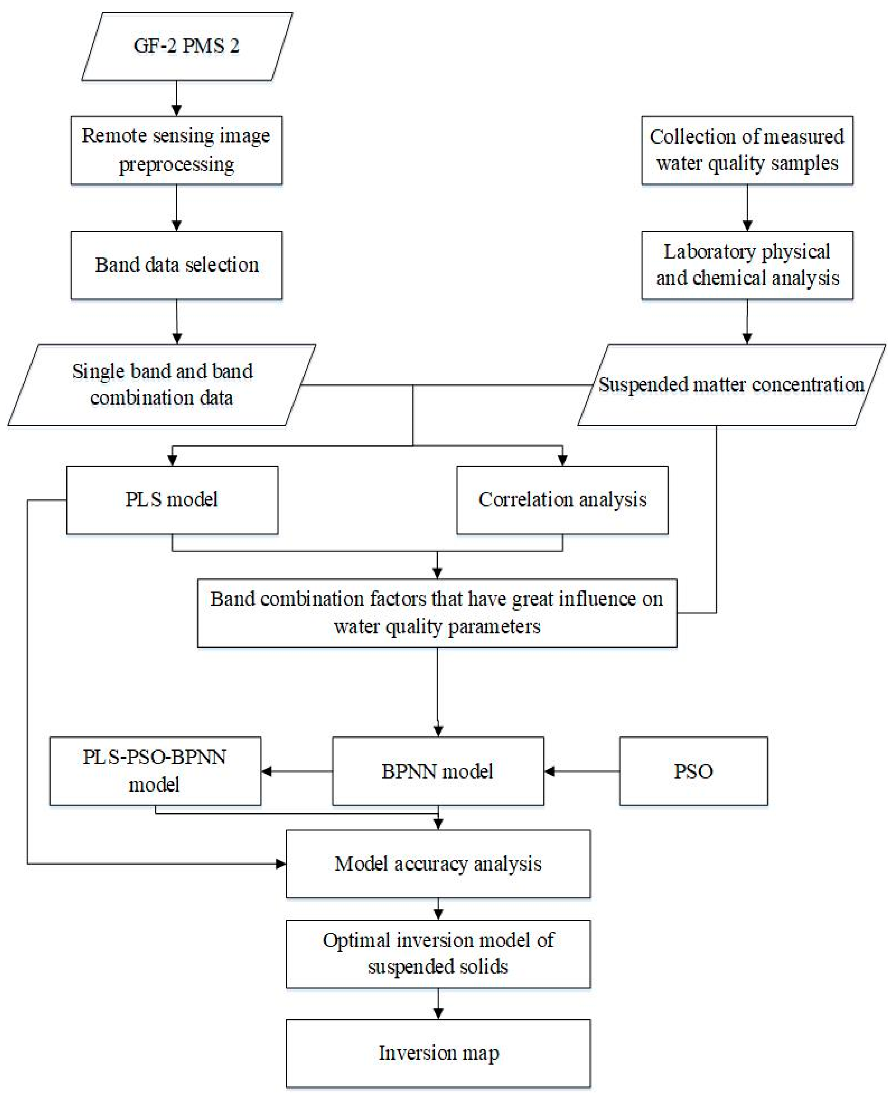
In order to improve the ability and efficiency of the algorithm for suspended matter concentration inversion, in this study an inversion model was built by optimizing the neural network with the partial least squares (PLS) algorithm and the particle swarm optimization algorithm. Based on the GF-2 remote sensing image data and the measured suspended matter concentration in the field, this study will integrate the partial least squares algorithm, the particle swarm optimization algorithm analysis and the BPNN to build a new and more accurate inversion model for the suspended matter concentration (
Figure 1).
2. Materials and Methodology
2.1. Study Area
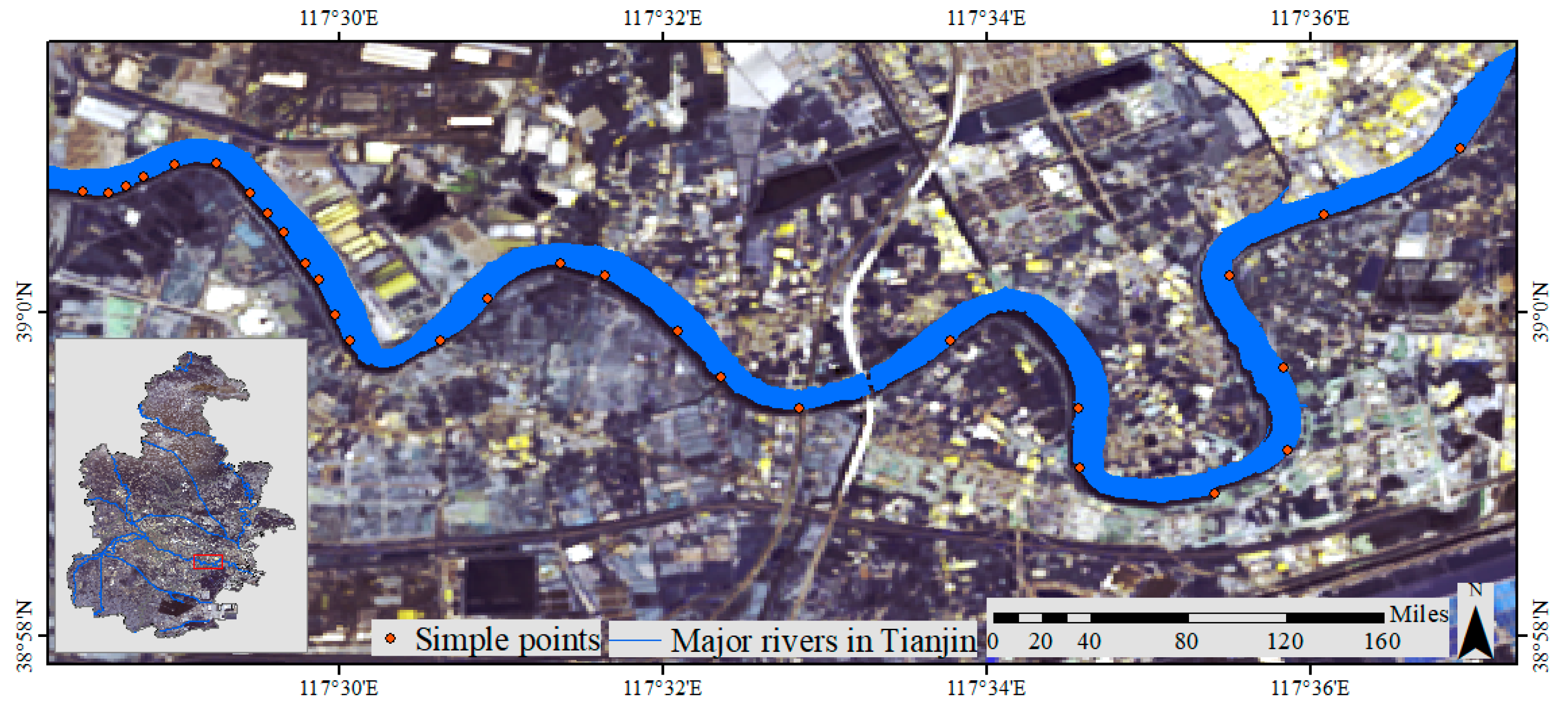
The Haihe water system is the largest water system in North China. It starts from the Zhanghe River as the source and ends at Dagukou flowing into the Bohai Bay, with a total length of 1031 km and a watershed area of 263,300 km
2. The study area is located in the lower reaches of the Haihe River (
Figure 2). It is mainly situated in the Binhai New Area of Tianjin.
2.2. Datasets
2.2.1. Remote Sensing Image Data
The GF-2 satellite is equipped with two high-resolution 1-m panchromatic and 4-m multispectral cameras, with a sub-meter spatial resolution, a high positioning accuracy and a fast attitude maneuverability. In this study, the 4-m-resolution multi-spectral CCD image acquired from PMS 2 sensor on 23 June 2019 was used. The image scene number was 4072610. The main image preprocessing included radiometric calibration, atmospheric correction, cropping and cloud removal. The gray values of the GF-2 PMS 2 image were calibrated with absolute calibration coefficients and radiometric calibration, using Equation (1).
where Le is the equivalent radiance at the entrance pupil of the satellite load channel, Gain and Bias are the gain and offset of the calibration coefficient, respectively and DN is the observation value of satellite load. The gain of the four bands of GF-2 PMS 2 was 0.1434, 0.1595, 0.1511 and 0.1685, respectively and the offsets were all 0.
After comparing a variety of methods, the Atmospheric Correction module was used for atmospheric correction. The longitude and latitude of the imaging center point were automatically obtained from the image by the fast line-of-sight atmospheric analysis of the spectral hypercubes model. The sensor height was 631 km and the pixel size was 4 m. The average height of the imaging area was set as the average altitude of Tianjin and the imaging time was automatically obtained. The atmospheric model and the aerosol model were finally confirmed as mid-latitude summer and Rural, based on the latitude, longitude and the image area. Due to the lack of short-wave infrared bands, the aerosol inversion method was set as None; the visibility was set to be 40 km; the spectral response function was downloaded from the “China Resources Satellite Application Center”; the block processing was set to be 100 m; the space subset outputs the panorama by default; and the output reflection range was 0~10,000.
2.2.2. Band Data
In this study, the BPNN model was the basis and its inversion accuracy was directly dependent on the input layer data. Based on the optical properties of the water quality parameters and using the partial least squares model, the influential wavelength factors on the water quality parameters were selected as the input layer data of the neural network model. The reflectance of pure water in the blue-green band was about 4%, the reflectance of the red band below 600 nm was significantly reduced, almost all of the incident energy was absorbed in the near-infrared and short-wave infrared parts and the reflectance of these bands was basically zero. However, there was no pure water in the surface water and many other substances contained in the water could have affected the reflectance of the water to a different extent. The spectral distribution of water is mainly influenced by chlorophyl a (Chl a) and suspended matter. Chl a and other pigment factors affect the reflectivity of water by absorbing incident light at different wavelengths, while suspended matter affects the reflectance of water through scattering incident light by solid particles suspended in the water. The scattering effect of the suspended matter increases the reflectance of the water within the whole wavelength. According to the correlation analysis of the band data and the measured suspended matter concentration, reflectance at the third band was used as the single-band data to invert the suspended matter concentration.
The combination of band data reduced the errors of the remote sensing image itself to a certain extent. Moreover, a reasonable combination of bands was used as an important input layer data of the neural network model. Previous studies have used the correlation coefficient between the band data and the measured water quality parameters as an important reference for the selection of neural network input values [
48]. It was found that there may be a nonlinear relationship between water quality parameters and remote sensing image data. However, the correlation coefficient is designed to evaluate the degree of linear correlation between the two variables. The neural network has a strong nonlinear fitting ability, so using the correlation coefficient to select data for the inversion of water quality parameters has some limitations. Considering the relatively high requirements of neural network modeling on the modeled samples, the partial least squares algorithm was able to combine and extract the information from the multi-dimensional independent variables to obtain the principal components, which had the strongest interpretation ability on the dependent variable and could summarize the information of the independent variables well. This effectively overcame the problem of multiple correlations between the variables and reduced the dimensionality of high-dimension data. In this study, the components were extracted through the partial least squares regression process and the principal components contributing to mutation information were screened out based on the covariance matrix by the principal component analysis process. This realizes the reduction in the screening and dimensionality in the large amount of band combination raw data. Then the screened components were used as input variables for the neural network to perform the neural network modeling.
2.2.3. Measured Water Quality Parameters
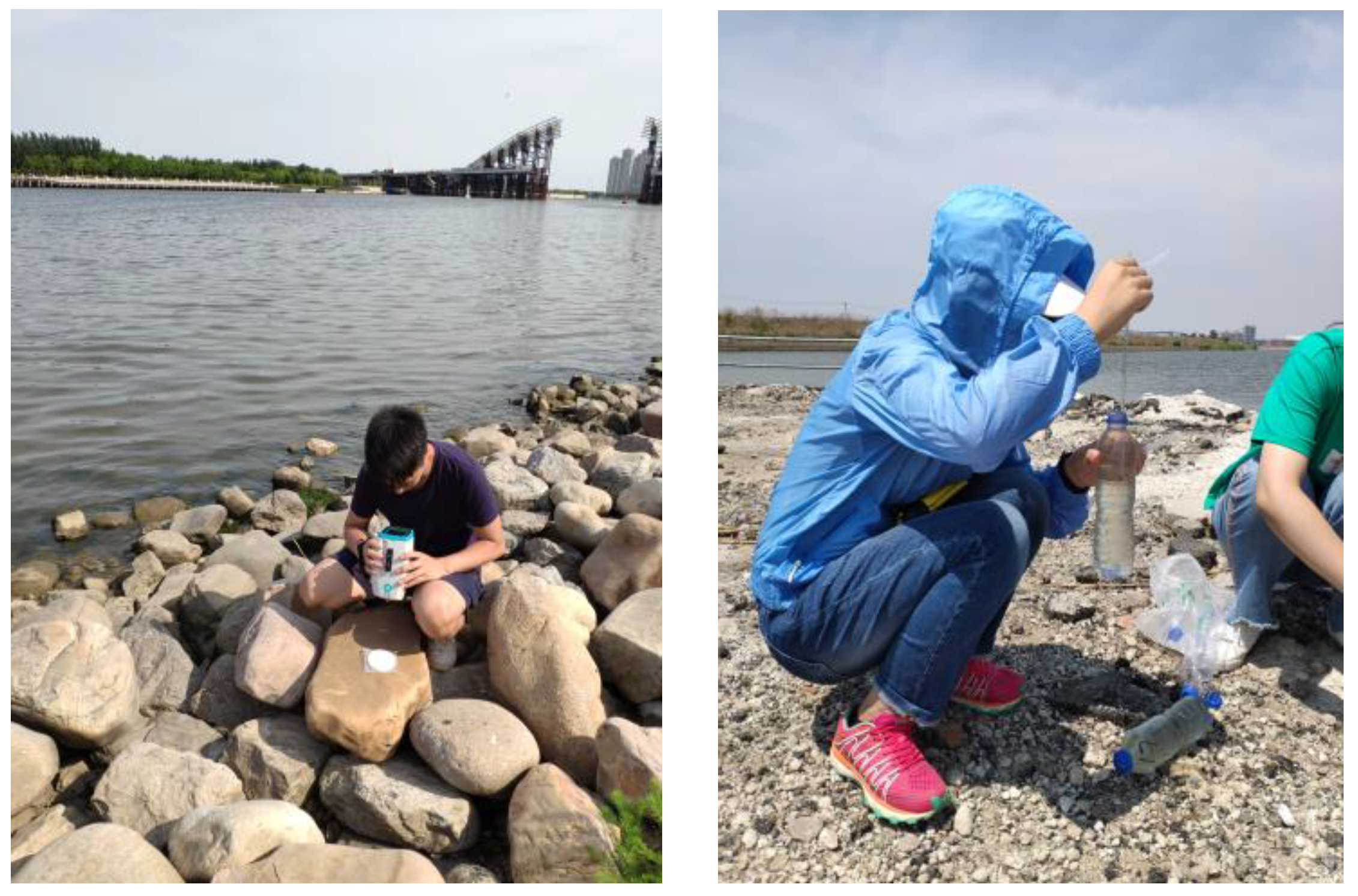
On 23 June 2019, a total of 41 sampling points were set and numbered from 1 to 41 along the Haihe river. Water samples were collected at each sampling point and the world geodetic system 1984 (WGS 84) coordinates of each sampling point were recorded using a handheld global positioning system (GPS). The water samples were processed by laboratory physicochemical analysis to obtain the suspended matter concentration.
Figure 3 shows photographs of the water samples collected in the field. The selected GF-2 remote sensing images only covered sampling points No. 1–29 on 23 June 2019, so the data from these 29 group images were used in the final analysis. Among them, 23 groups were used to build the inversion model for suspended matter concentration and the remaining 6 groups were used to validate the model.
2.3. Methods
It is understood that the change in water quality parameters is non-linear. The powerful learning ability of BPNN enables it to better fit the relationship between the remote sensing image data and the measured data; thus, it is a powerful tool to solve the nonlinear problem of water quality parameters. The partial least squares algorithm has advantages such as the objective interpretation of variables, support for a small number of samples and dimension reduction and it can be used as a method for screening neural network input values. The particle swarm optimization algorithm is a group intelligence algorithm designed to solve the problem of the global optimal solution, which can effectively mitigate the overfitting that exists in BPNN. Therefore, this study combined the partial least squares algorithm, the particle swarm optimization algorithm and BPNN to build an inversion model for suspended matter concentration. This model could effectively solve the overfitting and nonlinearity problems in suspended matter concentration inversion using remote sensing data and thus greatly improve the inversion accuracy.
2.3.1. Partial Least Squares Model
Partial least squares regression is a method for multivariate statistical regression analysis and can model many-to-many linear relationships [
49]. It is used when there are a large number of variables in two groups with multiple correlations but the number of observed samples is small. The modeling process is comprised of principal component analysis, typical correlation analysis and linear regression analysis. Therefore, besides building a more reasonable regression model, the analysis results include more rich and in-depth information derived from the above three methods. In this study, a partial least squares model was built using Matlab. On the one hand, the regression equation was solved and the suspended matter concentrations were inverted; on the other hand, the inversion results were used as the reference for screening the input layer data of neural network. The core code of the algorithm is listed below.
where X and Y are the independent and dependent variables, XL and YL are the loadings of the independent and dependent variables, XS and YS are the principal component score matrices, BETA is the final regression expression coefficient matrix, PCTVAR is the contribution of the corresponding principal component and MSE is the residual standard deviation matrix. Finally, the result is stored in the structure stats.
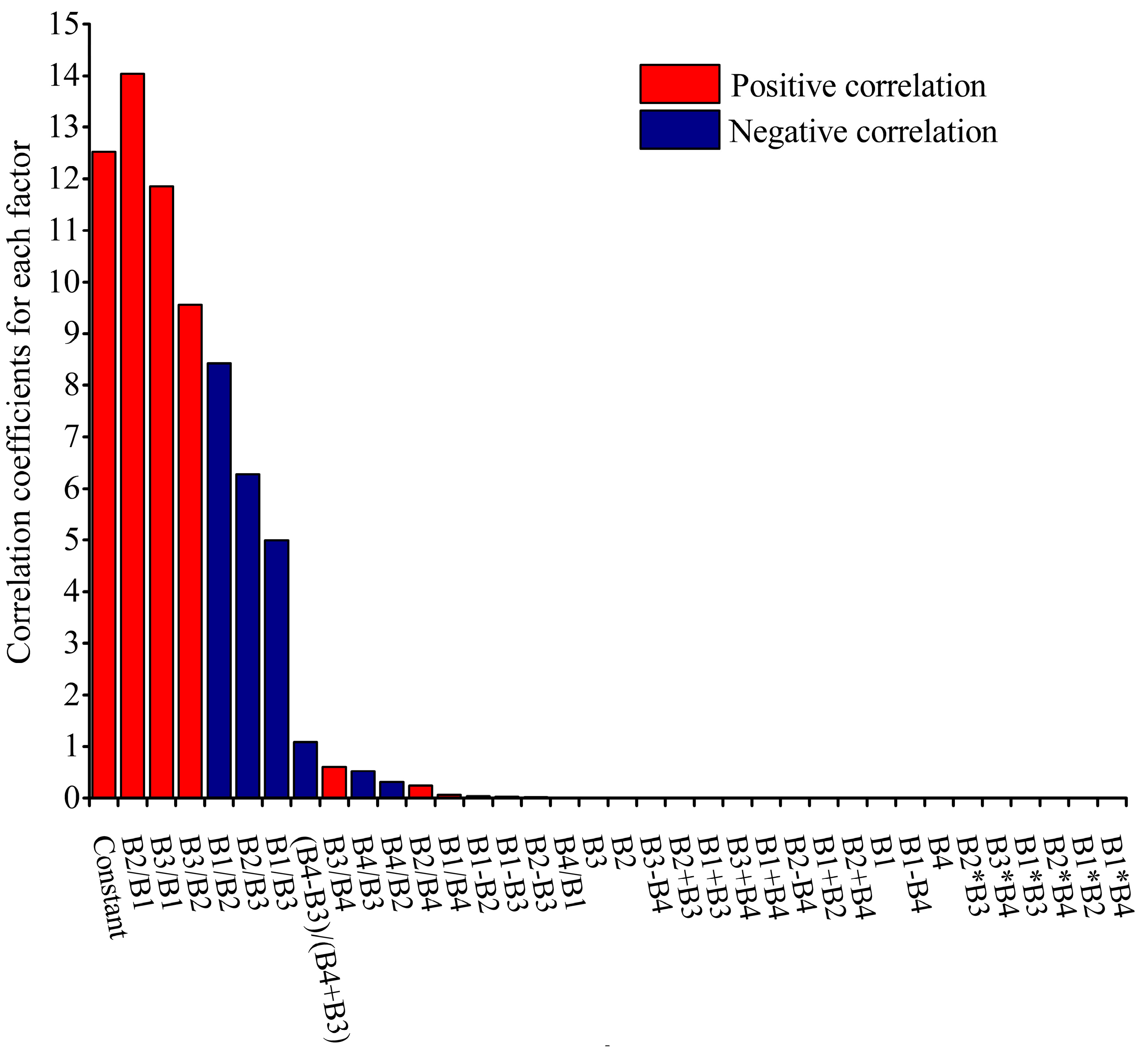
The coefficients of the factors in the partial least squares regression model are shown in
Figure 4. According to the regression results, B2/B1, B3/B1 and B3/B2 were positively correlated with the suspended matter concentration, while B1/B2, B2/B3 and B1/B3 were negatively correlated with the suspended matter concentration and played a decisive role in the regression model.
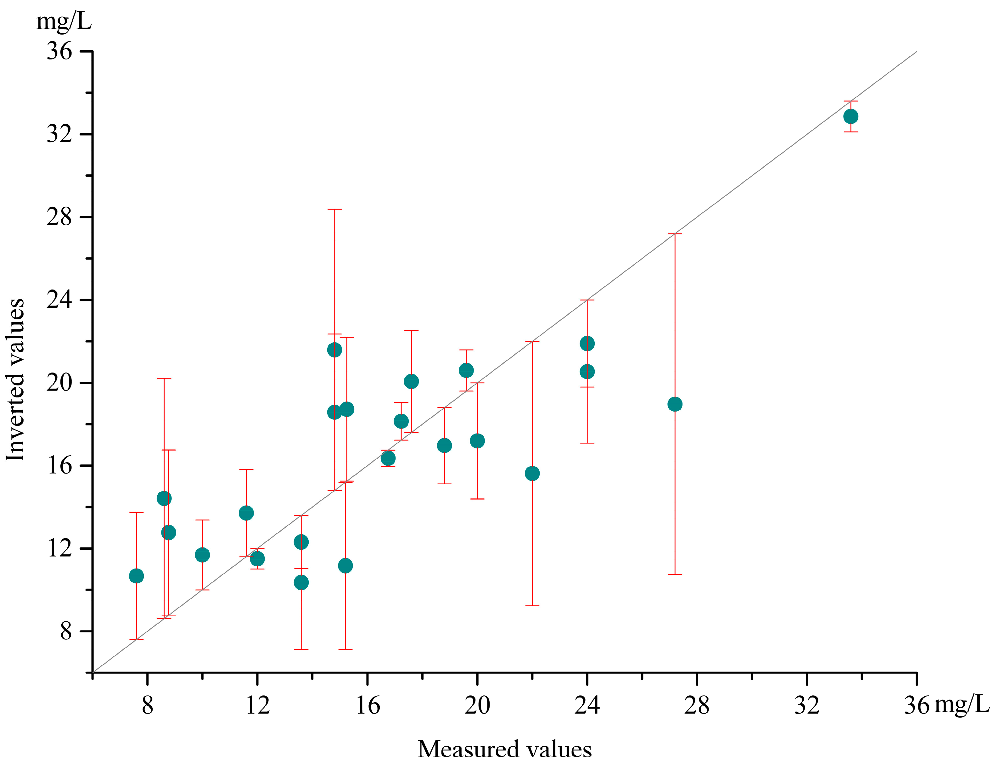
Figure 5 shows the deviation between the inverted values using the partial least squares regression model and the measured values. For this regression model, the absolute error was basically less than 4.0 mg/L and the root mean square error was 3.68 mg/L. The regression modelling results were used as the data selection criteria for the input layer of the neural network and the factors that played a major role in the partial least squares model were selected. In order to meet the diversity of data, a total of 8 sets of data including B3 and (B4 − B3)/(B4 + B3) were added as the input layer data to build the neural network inversion model.
2.3.2. BPNN Model
BPNN is a multilayer feedforward neural network trained using the error backpropagation algorithm and it is the most widely used in water quality parameter inversion. Its inversion accuracy is mainly affected by factors including the input data, the number of implicit layers, the implicit layer nodes and the choice of learning function. Therefore, to deal with different problems, corresponding improvement methods are adopted to obtain inversion results with higher accuracy. When building the neural network inversion model of water quality parameters, the input data were generally divided into the training set, the validation set and the test set. Considering the small amount of data, the neural network model was built by cross-validation using the leave-one-out method. Specifically, one of all the training samples was left at a time to complete the validation, then the average value of result was finally obtained after a repeated iteration, which was used as the judging standard for the model. To some extent, the use of this method mitigated the effect of the small sample size on the accuracy of BPNN inversion. BPNN consists of an input layer, a hidden layer and an output layer and the hidden layer can be further divided into a single hidden layer and multiple hidden layers according to the number of layers. Compared with single-hidden layer neural networks, multi-hidden layer neural networks have a longer training time, but their generalization ability is strong and their prediction accuracy is high. For complex mapping relationships, selecting multiple hidden layers can improve prediction accuracy. Generally, with the increase in the number of nodes, for simple function fitting, the neural network prediction error decreases; but for more complex problems, the network prediction error decreases and then increases. Therefore, the determination of the number of nodes is very important for the development of the neural network model. In practice, the selection of the number of nodes in the hidden layer affects the inversion effect of neural network training involving different data. This directly affects the accuracy of the water quality parameter inversion model and there is no exact criterion for the selection. If the number of hidden layer nodes is too small, the BPNN cannot establish a complex mapping relationship and the network prediction error is big; however, if the number of nodes is too large, the network learning time increases and overfitting may occur.
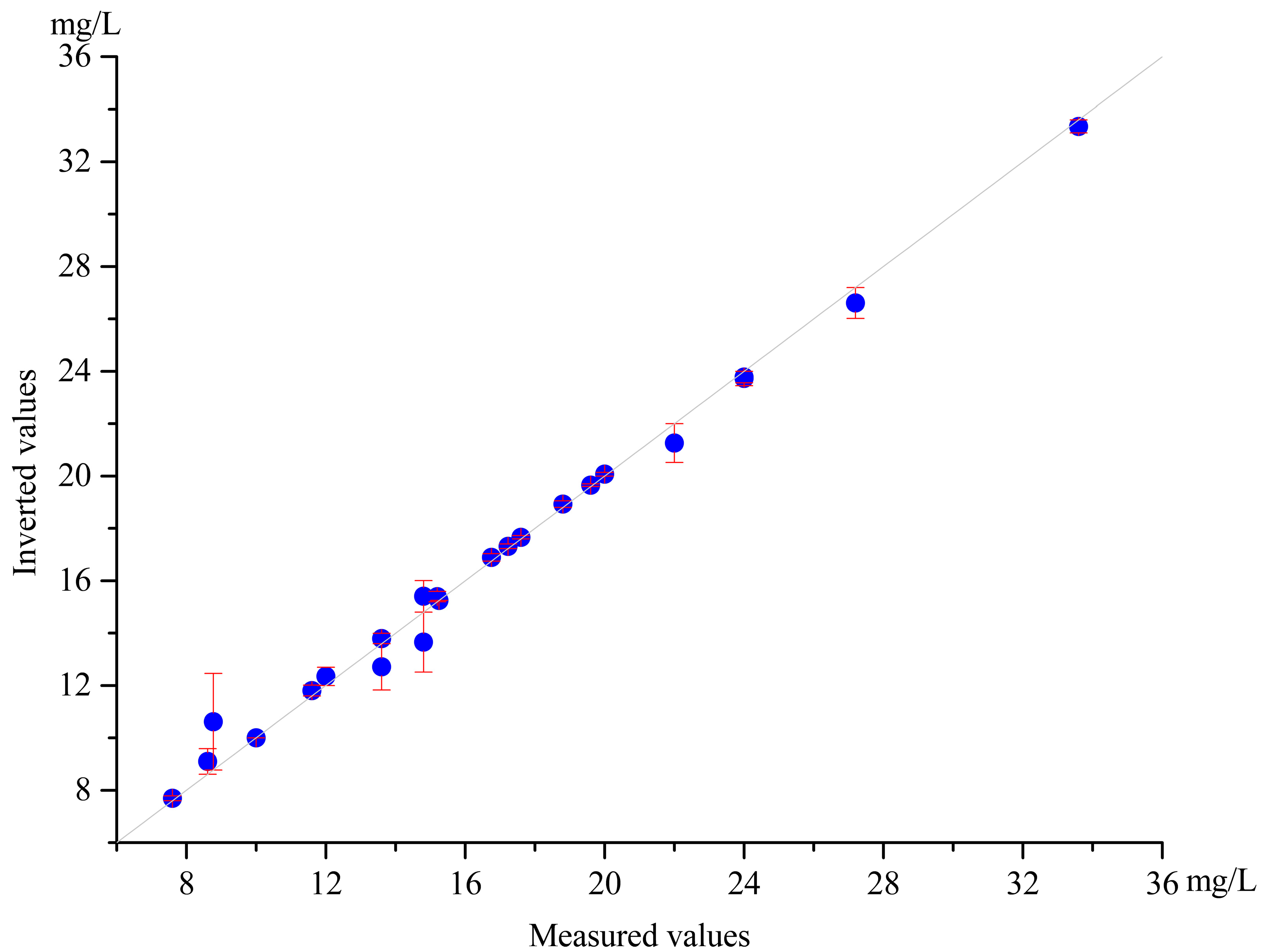
In order to obtain a higher inversion accuracy, this study built a neural network inversion model with two hidden layers. To determine a better node number of the hidden layer, the two hidden layer nodes were paired one by one from 1 to 23. Specifically, the number of neurons in the second hidden layer was fixed and the number of neurons in the first hidden layer was cycled in each test. According to the absolute error of the test, when the number of nodes in the second hidden layer is smaller than 3, the training neural network model is very unstable, the root mean square error of the training set fluctuates greatly and the absolute error of the test is very large; when the number of nodes in the second hidden layer is larger than 4, the root mean square error of the training set tends to be stable and the absolute error of the test gradually becomes smaller. Based on the above tests, the number of nodes in the second hidden layer was determined as 9. Similarly, the best training effect was obtained when the number of the first hidden layer node was 9. Thus, in this study, a two-hidden-layer neural network model, respectively, with the number of nodes as 9, was built. As shown in
Figure 6, the inverted value of the BPNN was basically consistent with the measured value with the error concentrated below 0.6 mg/L and the root mean square error of 0.57 mg/L. This is a big improvement in fitting over the partial least squares model (
Figure 6).
2.3.3. The Model Combines the PLS Algorithm and the PSO Algorithm to Optimize the BPNN Model
The neural network model greatly improved the accuracy of water quality parameter inversion due to its strong nonlinear fitting ability. However, it is prone to overfit, which limits the inversion accuracy of the BPNN model. The BPNN algorithm requires that the squared error of the expected value and the output value of all samples is less than a small given error allowed. The smaller the error, the higher the fitting accuracy and the higher the prediction accuracy of the network. As the fitting error decreases, the prediction error also decreases at the beginning; but when the fitting error decreases to a certain value, the prediction error increases instead, indicating that the generalization ability of the network is reduced. This is the overfitting phenomenon in the modeling of BPNN. Determination of the weights and thresholds of the neural network model is an important step in the BPNN modeling process, which is the determining factor of the learning process of the neural network. The optimization by particles using the particle swarm optimization algorithm could greatly improve the training accuracy and prediction ability of the neural network. The core of the particle swarm optimization algorithm is the collaboration between individuals in the group and the sharing of information. This determines an effective rule for the movement of particles in space and makes the movement of the whole group in space orderly. Finally, all the individuals in the group gather around the optimal solution and find the best solution, so as to solve the problems in the inversion of water quality parameters by neural networks and optimize the parameters of neural networks. The particle swarm optimization algorithm optimizes the neural network as follows: determining the feasible domain of the optimization problem, randomly scattering some particles into the feasible domain at the initial moment and assigning an initial random position and an initial random velocity to each particle. Then each particle’s position is advanced in turn according to its velocity, the known optimal global position in the problem space and the known optimal position of the particle. The d-dimension velocity update formula for each iteration of particle is shown in Equation (2). As the computation progresses, by using the known vantage point in the search space and the exploration of the next position, the particles gather or aggregate around one or more best points. The advantage of this algorithm is that it preserves the optimal global position and the known optimal position of the particles. These two pieces of information are effective for a faster convergence and for avoiding prematurely falling into local optimal solutions and they also lay the foundation for subsequent improvement of the BPNN inversion model using particle swarm optimization algorithms. The evaluation of the particle swarm optimization algorithm is shown in Equation (3).
where C
1 and C
2 are social learning factors and individual learning factors, R
1 and R
2 are random functions with the value range of [0, 1] to increase randomness of the search and W is the inertia weight to adjust the search range of the space.
In the previous section, the specific structural parameters of the input layer, hidden layer and output layer were determined. Then the data were added to be trained, the expected output values were given and the particle swarm optimization algorithm was added. The neural network model was optimized by the particle swarm optimization algorithm mainly through adjusting the weights and learning factors to solve the problem. The weights of the algorithm were adjusted by comparing the weights of linear decreasing weights, adaptive adjusting weights and stochastic weights. The learning factors of the particle swarm optimization algorithm were adjusted by comparing the contraction factors, synchronous learning factors and asynchronous learning factors. The parameters of the particle swarm optimization algorithm were initialized, including the velocity–displacement vector of the particles, the number of iterations, the learning factor and the inertia weights. From the tests, the parameters were finally set as follows: the number of particles was generally determined by the sample, which was set as 100; the learning factor corresponded to the group learning ability and self-learning ability of the particles, which were both set as 2.5. The weight affected the particle’s ability to update velocity, which was set to linearly decrease to adjust the weight. The adaptive function was set as the error function of the neural network.
The optimization processes were as follows. (1) The errors of the neural network were used as the fitness function of the particles, the fitness values of the particles were calculated and the individual extremes and the global optimal extremes were determined. (2) The velocity displacement of the particle was updated and calculated to obtain the particle fitness update value. (3) The individual and global extremes of the particles were repeatedly updated according to the new fitness values. (4) After repeated iterations, when the error reached the expected value or the iteration times reached the set maximum number, the particle swarm optimization algorithm was terminated and new neural network weights and thresholds were set based on the optimal result obtained.
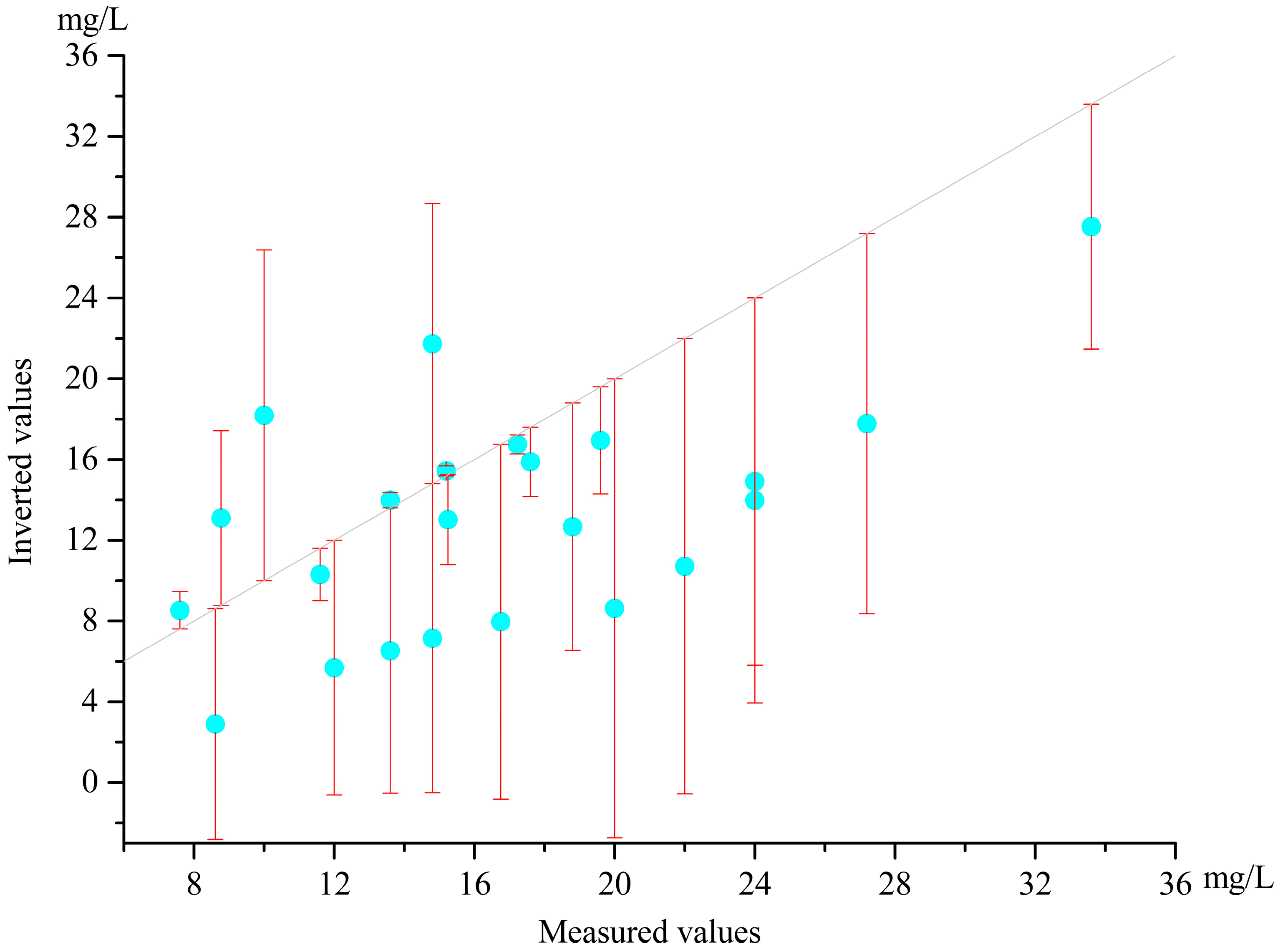
The inversion results of the BPNN model after optimization by the partial least squares algorithm and particle swarm optimization algorithm (PLS-PSO-BPNN) are shown in
Figure 7. The absolute error of PLS-PSO-BPNN model was increased to a certain extent compared with the BPNN model, with the root mean square error of 6.64 mg/L. It indicates that the PLS-PSO-BPNN model does not fit as well as the BPNN model and alleviates a certain degree of overfitting.
3. Results
In this study, the accuracy of the partial least squares model, the BPNN model and the optimized PLS-PSO-BPNN model were verified against the measured suspended matter concentration at six sampling sites, based on the absolute error, root mean square error, correlation coefficient and relative root mean square error. The absolute errors of the three inversion models at the sampling points are compared in
Figure 8.
Table 1 compares the errors of the training data and the test data of the three models. The root mean square error of the training data of the PLS-PSO-BPNN model was large, but the root mean square error of the test data was the smallest, which also reflects the overfitting phenomenon of the BPNN model. It shows that the inversion model based on the partial least squares algorithm had a larger absolute error, while the accuracy of the BPNN inversion model was greatly improved. It indicates that the inversion model built by BPNN can be well applied to the remote sensing inversion of suspended matter concentration. Moreover, the PLS-PSO-BPNN model, to which both the partial least squares and the particle swarm optimization algorithm were added on the basis of the traditional neural network model, improved the accuracy of suspended matter concentration inversion to some extent.
By comparing the errors between the inversion values and the measured values of the training set and the verification set based on the three models, it was found that the inversion results of the two neural network models were far superior to the partial least squares model, which proves the advantages of the neural network applied to water quality parameters. Among the three inversion models, the BPNN had the best fitting of the training set, but the fitting degree of the validation set was not the best, mainly because the BPNN had serious fitting when the suspended matter concentration inversion model was constructed, which led to a deviation in the predicted value of the verification point and a decrease in accuracy. This was also the problem to be solved by introducing the particle swarm optimization algorithm. From the experimental results, the PLS-PSO-BPNN model improved the inversion accuracy of water quality parameters.
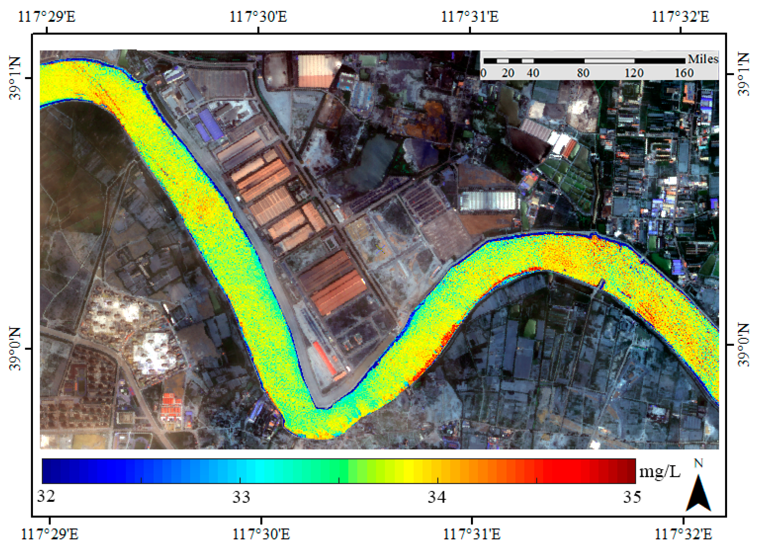
The PLS-PSO-BPNN model was applied to invert the suspended matter concentration in the formed waters and the results are shown in
Figure 9. The brighter the color of the grid, the higher the concentration of suspended matter. A high concentrations of suspended solids was observed in the waters adjacent to the southern shore.
4. Discussion
Remote sensing technology used in water quality parameter inversion is affected by many factors. First, remote sensing images are limited by the spatial resolution, spectral resolution and temporal resolution. Second, topography, climate, seasons and other factors also affect the accuracy of the remote sensing inversion of water quality parameters to some extent. Third, the water body itself is a complex system. Waters in different areas and different seasons show different states. The number of water quality parameters in water is much more than expected and different water quality parameters interact with each other, which makes the water environment very complex. A large number of previous studies have successfully applied remote sensing technology in the water quality parameter inversion. However, due to the complexity of the water environment, the relationship between spectral reflectance and water quality parameters is nonlinear. The development of traditional linear regression models is insufficient to perform an accurate inversion of water quality parameters. Therefore, to mitigate the effect of the above factors, the main focus of the remote sensing inversion of water quality parameter is improving the inversion accuracy.
Compared with previous studies, the main improvements of this study are reflected in the following aspects. First, this study found that the BPNN greatly improved the accuracy of the remote sensing inversion of suspended matter concentration, compared with the statistical regression model. The inversion accuracy increased from 9.50 mg/L to 4.04 mg/L. Second, to tackle the over-fitting problem of BPNN, this study used the particle swarm optimization algorithm to optimize the weight and threshold of BPNN, which effectively avoids the problem that BPNN can easily to fall into, creating the local optimal solution and thereby improving the inversion accuracy of suspended matter concentration by the neural network. The relative errors of the results were reduced overall and the variance of the corresponding results of the model was also relatively reduced. This indicates that the inversion using the neural network model optimized by the particle swarm optimization algorithm was more accurate and more stable. Third, the screening rule of the BPNN input layer data is always lacking a theoretical basis. This study introduced the partial least squares algorithm into the screening of the neural network input layer data, which provided a more scientific insight on this process. Fourth, it was proven that the improved PLS-PSO-BPNN model optimized by partial least squares algorithm and particle swarm optimization algorithm had a good performance in the inversion of suspended matter concentration. This improved model can provide a methodological reference for the inversion of suspended matter concentration in other regions.
5. Conclusions
This study demonstrated the feasibility of using high-resolution remote sensing images to perform a rapid assessment of suspended matter concentration inversion. It developed an optimized neural network model based on the partial least squares algorithm and the particle swarm optimization algorithm, the PLS-PSO-BPNN model and used the measured suspended matter concentration data and GF-2 remote sensing image data to invert suspended matter concentration of suspended matter.
The inversion results indicated that the accuracy was very high. In this model, the partial least squares algorithm can extract neural network input values more scientifically and optimize the selection rules of neural network input values. The particle swarm optimization algorithm could handle the over-fitting problem of neural network and optimize the neural network model.
In this study, the particle swarm optimization neural network model was used and the partial least squares method was introduced to the original neural network input value selection method, which further improved the suspended matter concentration inversion accuracy and the theoretical basis of the inversion method. It can be seen that compared with the traditional BPNN and the partial least squares inversion model, the PLS-PSO-BPNN model combined the partial least squares algorithm and the particle swarm optimization algorithm and its inversion accuracy of the remote sensing image was significantly higher. First, this proved the outstanding advantages of BPNN algorithm in the research of water quality parameter remote sensing inversion. Secondly, the proposed BPNN algorithm provides a new idea for improving the accuracy of water quality parameter remote sensing inversion by not only dealing with the problems of the neural network algorithm in the actual water quality parameter inversion, but also being optimized to overcome limitations of its own algorithm. Finally, even under the influence of various complex factors such as water, seasons and images, the algorithm was able to perform a fast and accurate inversion of the water quality parameters in large areas of water through corresponding parameter adjustment.
Author Contributions
All of the authors have contributed extensively to the work. Design of the research, Q.G.; establishing model, H.W.; analyzing data, H.J.; processing data, G.Y.; substantial revision of the manuscript, X.W. All authors were involved in writing and revising the manuscript. All authors have read and agreed to the published version of the manuscript.
Funding
This work was supported by the Scientific Research Project of Tianjin municipal Education Commission, China (grant number No. 2020KJ051) and the National Natural Science Foundation of China, grant number (grant number No. 41971310).
Institutional Review Board Statement
Not applicable.
Informed Consent Statement
Not applicable.
Data Availability Statement
The data presented in this study are available on request from the corresponding author.
Conflicts of Interest
The authors declare no conflict of interest.
References
- Cao, H.; Han, L.; Li, W.; Liu, Z.; Li, L. Inversion and distribution of total suspended matter in water based on remote sensing images—A case study on Yuqiao Reservoir, China. Water Environ. Res. 2021, 93, 582–595. [Google Scholar] [CrossRef] [PubMed]
- Wang, C.; Chen, S.; Li, D.; Wang, D.; Liu, W.; Yang, J. A Landsat-based model for retrieving total suspended solids concentration of estuaries and coasts in China. Geosci. Model Dev. 2017, 10, 4347–4365. [Google Scholar] [CrossRef] [Green Version]
- Wang, H.; Wang, J.; Cui, Y.; Yan, S. Consistency of Suspended Particulate Matter Concentration in Turbid Water Retrieved from Sentinel-2 MSI and Landsat-8 OLI Sensors. Sensors 2021, 21, 1662. [Google Scholar] [CrossRef] [PubMed]
- Tyler, A.N.; Hunter, P.D.; Spyrakos, E.; Groom, S.; Constantinescu, A.M.; Kitchen, J. Developments in Earth observation for the assessment and monitoring of inland, transitional, coastal and shelf-sea waters. Sci. Total Environ. 2016, 572, 1307–1321. [Google Scholar] [CrossRef] [Green Version]
- Shang, W.; Jin, S.; He, Y.; Zhang, Y.; Li, J. Spatial–Temporal Variations of Total Nitrogen and Phosphorus in Poyang, Dongting and Taihu Lakes from Landsat-8 Data. Water 2021, 13, 1704. [Google Scholar] [CrossRef]
- He, Y.; Gong, Z.; Zheng, Y.; Zhang, Y. Inland Reservoir Water Quality Inversion and Eutrophication Evaluation Using BP Neural Network and Remote Sensing Imagery: A Case Study of Dashahe Reservoir. Water 2021, 13, 2844. [Google Scholar] [CrossRef]
- Feng, L.; Hu, C.; Chen, X.; Song, Q. Influence of the Three Gorges Dam on total suspended matters in the Yangtze Estuary and its adjacent coastal waters: Observations from MODIS. Remote Sens. Environ. 2004, 140, 779–788. [Google Scholar] [CrossRef]
- Hui, J.; Yao, L. Analysis and inversion of the nutritional status of China’s Poyang Lake using MODIS data. J. Indian Soc. Remote Sens. 2016, 44, 837–842. [Google Scholar] [CrossRef]
- Xiong, J.; Lin, C.; Ma, R.; Cao, Z. Remote sensing estimation of lake total phosphorus concentration based on MODIS: A case study of Lake Hongze. Remote Sens. 2019, 11, 2068. [Google Scholar] [CrossRef] [Green Version]
- Papoutsa, C.; Retalis, A.; Toulios, L.; Hadjimitsis, D.G. Defining the Landsat TM/ETM+ and CHRIS/PROBA spectral regions in which turbidity can be retrieved in inland waterbodies using field spectroscopy. Int. J. Remote Sens. 2014, 35, 1674–1692. [Google Scholar] [CrossRef]
- Cai, L.; Tang, D.; Li, C. An investigation of spatial variation of suspended sediment concentration induced by a bay bridge based on Landsat TM and OLI data. Adv. Space Res. 2015, 56, 293–303. [Google Scholar] [CrossRef]
- González-Márquez, L.C.; Torres-Bejarano, F.M.; Rodríguez-Cuevas, C.; Torregroza-Espinosa, A.C.; Sandoval-Romero, J.A. Estimation of water quality parameters using Landsat 8 images: Application to Playa Colorada Bay, Sinaloa, Mexico. Appl. Geomat. 2018, 10, 147–158. [Google Scholar] [CrossRef]
- Kuan, H.; Li, J.; Zhang, X.; Zhang, J.; Cui, H.; Sun, Q. Remote Estimation of Water Quality Parameters of Medium-and Small-Sized Inland Rivers Using Sentinel-2 Imagery. Water 2020, 12, 3124. [Google Scholar]
- Peterson, K.T.; Sagan, V.; Sloan, J.J. Deep learning-based water quality estimation and anomaly detection using Landsat-8/Sentinel-2 virtual constellation and cloud computing. Gisci. Remote Sens. 2020, 57, 510–525. [Google Scholar] [CrossRef]
- Sent, G.; Biguino, B.; Favareto, L.; Cruz, J.; Sa, C.; Dogliotti, A.I.; Palma, C.; Brotas, V.; Brito, A.C. Deriving Water Quality Parameters Using Sentinel-2 Imagery: A Case Study in the Sado Estuary, Portugal. Remote Sens. 2021, 13, 1043. [Google Scholar] [CrossRef]
- Xu, J.; Gao, C.; Wang, Y. Extraction of Spatial and Temporal Patterns of Concentrations of Chlorophyll-a and Total Suspended Matter in Poyang Lake Using GF-1 Satellite Data. Remote Sens. 2020, 12, 622. [Google Scholar] [CrossRef] [Green Version]
- Lu, S.; Deng, R.; Liang, Y.; Xiong, L.; Ai, X.; Qin, Y. Remote Sensing Retrieval of Total Phosphorus in the Pearl River Channels Based on the GF-1 Remote Sensing Data. Remote Sens. 2020, 12, 1420. [Google Scholar] [CrossRef]
- Zeng, S.; Li, Y.; Lyu, H.; Xu, J.; Dong, X.; Wang, R.; Yang, Z.; Li, J. Mapping spatio-temporal dynamics of main water parameters and understanding their relationships with driving factors using GF-1 images in a clear reservoir. Environ. Sci. Pollut. R. 2020, 27, 33929–33950. [Google Scholar] [CrossRef]
- Zhang, Y.; Wu, L.; Ren, H.; Deng, L.; Zhang, P. Retrieval of Water Quality Parameters from Hyperspectral Images Using Hybrid Bayesian Probabilistic Neural Network. Remote Sens. 2020, 12, 1567. [Google Scholar] [CrossRef]
- Niroumand-Jadidi, M.; Bovolo, F.; Bruzzone, L. Water Quality Retrieval from PRISMA Hyperspectral Images: First Experience in a Turbid Lake and Comparison with Sentinel-2. Remote Sens. 2020, 12, 3984. [Google Scholar] [CrossRef]
- Zhang, Y.; Wu, L.; Ren, H.; Liu, Y.; Zheng, Y.; Liu, Y.; Dong, J. Mapping water quality parameters in urban rivers from hyperspectral images using a new self-adapting selection of multiple artificial neural networks. Remote Sens. 2020, 12, 336. [Google Scholar] [CrossRef] [Green Version]
- Wang, X.; Yang, W. Water quality monitoring and evaluation using remote sensing techniques in China: A systematic review. Ecosyst. Health Sustain. 2019, 5, 47–56. [Google Scholar] [CrossRef] [Green Version]
- Hafeez, S.; Wong, M.S.; Ho, H.C.; Nazeer, M.; Nichol, J.; Abbas, S.; Tang, D.; Lee, K.; Pun, L. Comparison of machine learning algorithms for retrieval of water quality indicators in case-II waters: A case study of Hong Kong. Remote Sens. 2019, 11, 617. [Google Scholar] [CrossRef] [Green Version]
- Wei, L.; Huang, C.; Zhong, Y.; Wang, Z.; Hu, X.; Lin, L. Inland waters suspended solids concentration retrieval based on PSO-LSSVM for UAV-borne hyperspectral remote sensing imagery. Remote Sens. 2019, 11, 1455. [Google Scholar] [CrossRef] [Green Version]
- Tavora, J.; Boss, E.S.; Doxaran, D.; Hill, P. An algorithm to estimate suspended particulate matter concentrations and associated uncertainties from remote sensing reflectance in coastal environments. Remote Sens. 2020, 12, 2172. [Google Scholar] [CrossRef]
- Ruždjak, A.M.; Ruždjak, D. Evaluation of river water quality variations using multivariate statistical techniques. Environ. Monit. Assess. 2015, 187, 215. [Google Scholar]
- Saikrishna, K.; Purushotham, D.; Sunitha, V.; Reddy, Y.S.; Linga, D.; Kumar, B.K. Data for the evaluation of groundwater quality using water quality index and regression analysis in parts of Nalgonda district, Telangana, Southern India. Data Brief 2020, 32, 106235. [Google Scholar] [CrossRef]
- Parmar, K.S.; Bhardwaj, R. River water prediction modeling using neural networks, fuzzy and wavelet coupled model. Water Resour. Manag. 2015, 29, 17–33. [Google Scholar] [CrossRef]
- Heddam, S. Secchi disk depth estimation from water quality parameters: Artificial neural network versus multiple linear regression models? Environ. Process. 2016, 3, 525–536. [Google Scholar] [CrossRef]
- Pu, F.; Ding, C.; Chao, Z.; Yu, Y.; Xu, X. Water-quality classification of inland lakes using Landsat8 images by convolutional neural networks. Remote Sens. 2019, 11, 1674. [Google Scholar] [CrossRef] [Green Version]
- Godo-Pla, L.; Emiliano, P.; Valero, F.; Poch, M.; Sin, G.; Monclús, H. Predicting the oxidant demand in full-scale drinking water treatment using an artificial neural network: Uncertainty and sensitivity analysis. Process Saf. Environ. 2019, 125, 317–327. [Google Scholar] [CrossRef]
- Xue, K.; Ma, R.; Duan, H.; Shen, M.; Boss, E.; Cao, Z. Inversion of inherent optical properties in optically complex waters using sentinel-3A/OLCI images: A case study using China’s three largest freshwater lakes. Remote Sens. Environ. 2019, 225, 328–346. [Google Scholar] [CrossRef]
- Yan, X.; Gong, J.Y.; Wu, Q. Pollution source intelligent location algorithm in water quality sensor networks. Neural Comput. Appl. 2020, 33, 209–222. [Google Scholar] [CrossRef]
- Mohammadi, B.; Guan, Y.; Moazenzadeh, R.; Safari, M.J.S. Implementation of hybrid particle swarm optimization-differential evolution algorithms coupled with multi-layer perceptron for suspended sediment load estimation. Catena 2021, 198, 105024. [Google Scholar] [CrossRef]
- Sagan, V.; Peterson, K.T.; Maimaitijiang, M.; Sidike, P.; Sloan, J.; Greeling, B.A.; Maalouf, S.; Adams, C. Monitoring inland water quality using remote sensing: Potential and limitations of spectral indices, bio-optical simulations, machine learning, and cloud computing. Earth-Sci. Rev. 2020, 205, 103187. [Google Scholar] [CrossRef]
- Chang, F.J.; Tsai, Y.H.; Chen, P.A.; Coynel, A.; Vachaud, G. Modeling water quality in an urban river using hydrological factors–Data driven approaches. J. Environ. Manag. 2015, 151, 87–96. [Google Scholar] [CrossRef]
- Singh, B.; Sihag, P.; Singh, K. Modelling of impact of water quality on infiltration rate of soil by random forest regression. Model. Earth Syst. Environ. 2017, 3, 999–1004. [Google Scholar] [CrossRef]
- Ramo, R.; Chuvieco, E. Developing a random forest algorithm for MODIS global burned area classification. Remote Sens. 2017, 9, 1193. [Google Scholar] [CrossRef] [Green Version]
- Haag, T.; Herrmann, J.; Hanss, M. Identification procedure for epistemic uncertainties using inverse fuzzy arithmetic. Mech. Syst. Signal Processing 2010, 24, 2021–2034. [Google Scholar] [CrossRef]
- Nadiri, A.A.; Shokri, S.; Tsai, F.T.C.; Moghaddam, A.A. Prediction of effluent quality parameters of a wastewater treatment plant using a supervised committee fuzzy logic model. J. Clean. Prod. 2018, 180, 539–549. [Google Scholar] [CrossRef]
- Bozorg-Haddad, O.; Soleimani, S.; Loaiciga, H. Modeling water-quality parameters using genetic algorithm–least squares support vector regression and genetic programming. J. Environ. Eng. 2017, 143, 04017021. [Google Scholar] [CrossRef]
- Wang, J.; Fu, Z.; Qiao, H.; Liu, F. Assessment of eutrophication and water quality in the estuarine area of Lake Wuli, Lake Taihu, China. Sci. Total Environ. 2018, 650, 1392–1402. [Google Scholar] [CrossRef] [PubMed]
- Dahlén, J.; Karlsson, S.; Bäckström, M.; Hagberg, J.; Pettersson, H. Determination of nitrate and other water quality parameters in groundwater from UV/V is spectra employing partial least squares regression. Chemosphere 2000, 40, 71–77. [Google Scholar] [CrossRef]
- Wang, Z.; Kawamura, K.; Sakuno, Y.; Fan, X.; Gong, Z.; Lim, J. Retrieval of chlorophyll-a and total suspended solids using iterative stepwise elimination partial least squares (ISE-PLS) regression based on field hyperspectral measurements in irrigation ponds in Higashihiroshima, Japan. Remote Sens. 2017, 9, 264. [Google Scholar] [CrossRef] [Green Version]
- Yan, J.; Xu, Z.; Yu, Y.; Xu, H.; Gao, K. Application of a hybrid optimized BP network model to estimate water quality parameters of Beihai Lake in Beijing. Appl. Sci. 2019, 9, 1863. [Google Scholar] [CrossRef] [Green Version]
- Tharwat, A.; Hassanien, A.E. Quantum-behaved particle swarm optimization for parameter optimization of support vector machine. J. Classif. 2019, 36, 576–598. [Google Scholar] [CrossRef]
- Thea, V.R.; Peabody, M.A.; Uyaguari-Diaz, M.I.; Cronin, K.I.; Chan, M.; Slobodan, J.R.; Nesbitt, M.J.; Suttle, C.A.; Hsiao, W.W.L.; Tang, P.K.C.; et al. Year-long metagenomic study of river microbiomes across land use and water quality. Front. Microbiol. 2015, 6, 1405. [Google Scholar]
- Din, E.S.E.; Zhang, Y.; Suliman, A. Mapping concentrations of surface water quality parameters using a novel remote sensing and artificial intelligence framework. Int. J. Remote Sens. 2017, 38, 1023–1042. [Google Scholar]
- Elsayed, S.; Gad, M.; Farouk, M.; Saleh, A.H.; Hussein, H.; Elmetwalli, A.H.; Elsherbiny, O.; Moghanm, F.S.; Moustapha, M.E.; Taher, M.A.; et al. Using Optimized Two and Three-Band Spectral Indices and Multivariate Models to Assess Some Water Quality Indicators of Qaroun Lake in Egypt. Sustainability 2021, 13, 10408. [Google Scholar] [CrossRef]
| Publisher’s Note: MDPI stays neutral with regard to jurisdictional claims in published maps and institutional affiliations. |
© 2022 by the authors. Licensee MDPI, Basel, Switzerland. This article is an open access article distributed under the terms and conditions of the Creative Commons Attribution (CC BY) license (https://creativecommons.org/licenses/by/4.0/).


