Effect of Battery-Electric and Plug-In Hybrid Electric Vehicles on PM2.5 Emissions in 29 European Countries

Abstract

The contribution of battery electric vehicles (BEVs) and plug-in hybrid electric vehicles (PHEVs) to mitigating/reducing fine particulate matter (PM2.5) emissions was researched through a panel of 29 European countries from 2010 to 2019, using the econometric technique of method of moments quantile regression (MM-QR). This research is innovative by connecting the increasing use of electric vehicles with PM2.5 emissions and using the MM-QR to explore this relationship. Two models were estimated to analyse their contribution to reducing PM2.5 in European countries. The nonlinearity of the models were confirmed. The statistical significance of the variables is strong for the upper quantiles (75th and 90th), resulting from the effectiveness of European policies to improve the environment. Electric vehicles (BEVs and PHEVs), economic growth, and urbanisation reduce the PM2.5 problem, but energy intensity and fossil fuel consumption aggravate it. This research sheds light on how policymakers and governments can design proposals to encourage electric vehicle use in European countries. To achieve the long-term climate neutral strategy by 2050, it is imperative to implement effective policies to reduce the consumption of fossil fuels and promote the adoption of electric vehicles using renewable energy sources.

1. Introduction

Many cities suffer from poor air quality in Europe. As a result, they frequently exceed the European Union’s (EU) Air Quality Framework Directive 96/62/EC and its daughter directives and guidelines recommended by the World Health Organization (WHO). This issue is fine particulate matter (PM1.0), for which the daily rate of 50 µg/m³ is not to be exceeded on more than 35 days a year. Indeed, in the many cities and regions in Europe, the yearly average limit values (40 µg/m³) are often exceeded [1]. However, the minimum threshold of particulate matter below which there are no adverse health effects could not be established. The WHO guidelines represent global targets (for both industrialised and developing countries) above which increased mortality responses because of particulate matter air pollution are expected based on current scientific findings (e.g., Thunis et al. [1] and WHO [2]). In the case of particulate matter (PM2.5), the EU limited value is an annual average of 25 µg/m³ [1]. 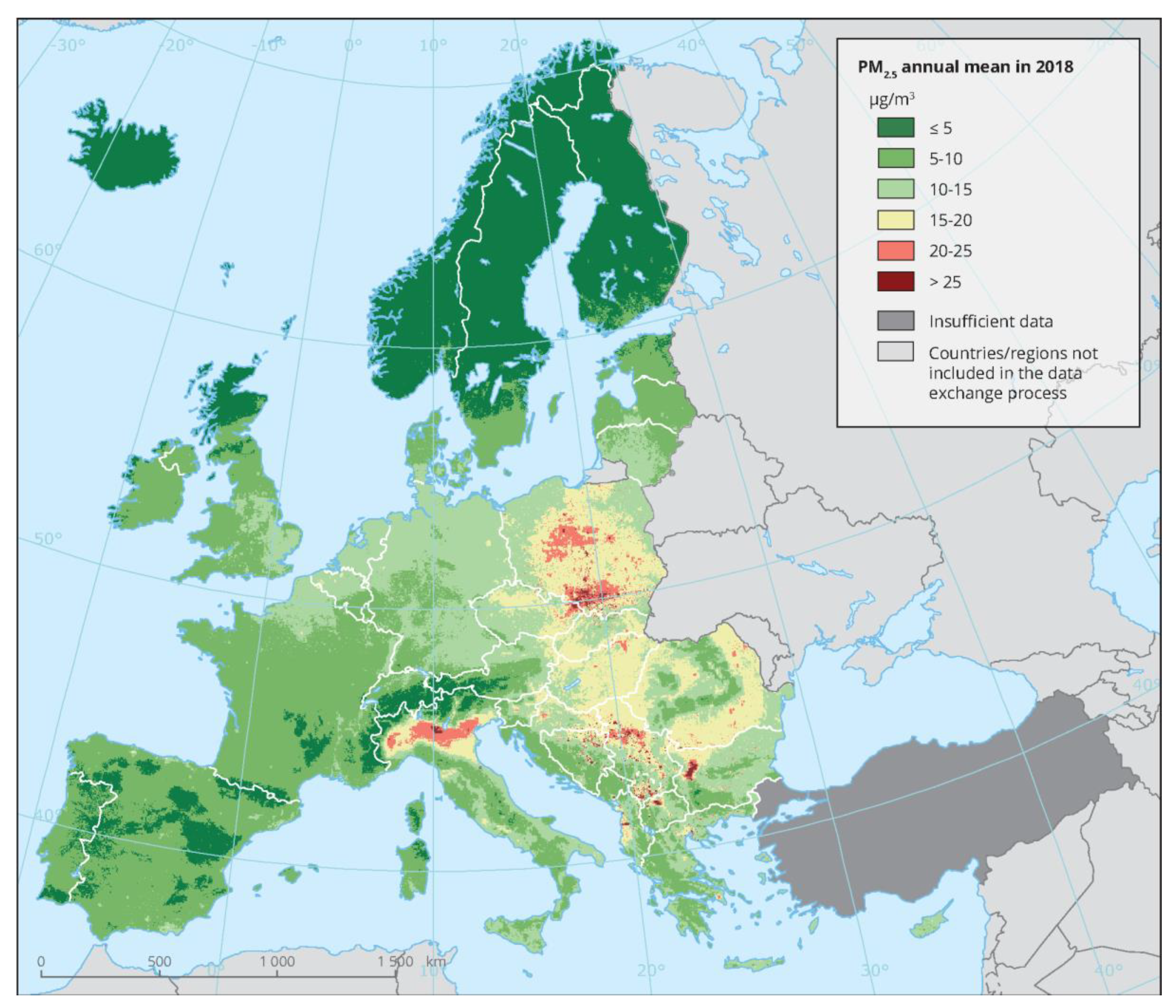This target was established through Ambient Air Quality Directive 2008/50/EC that settled particulate matter (PM2.5) [3]. However, few cities across the EU have managed to keep concentrations below the WHO’s recommended level (10 µg/m³ on an annual basis), as illustrated in Figure 1.

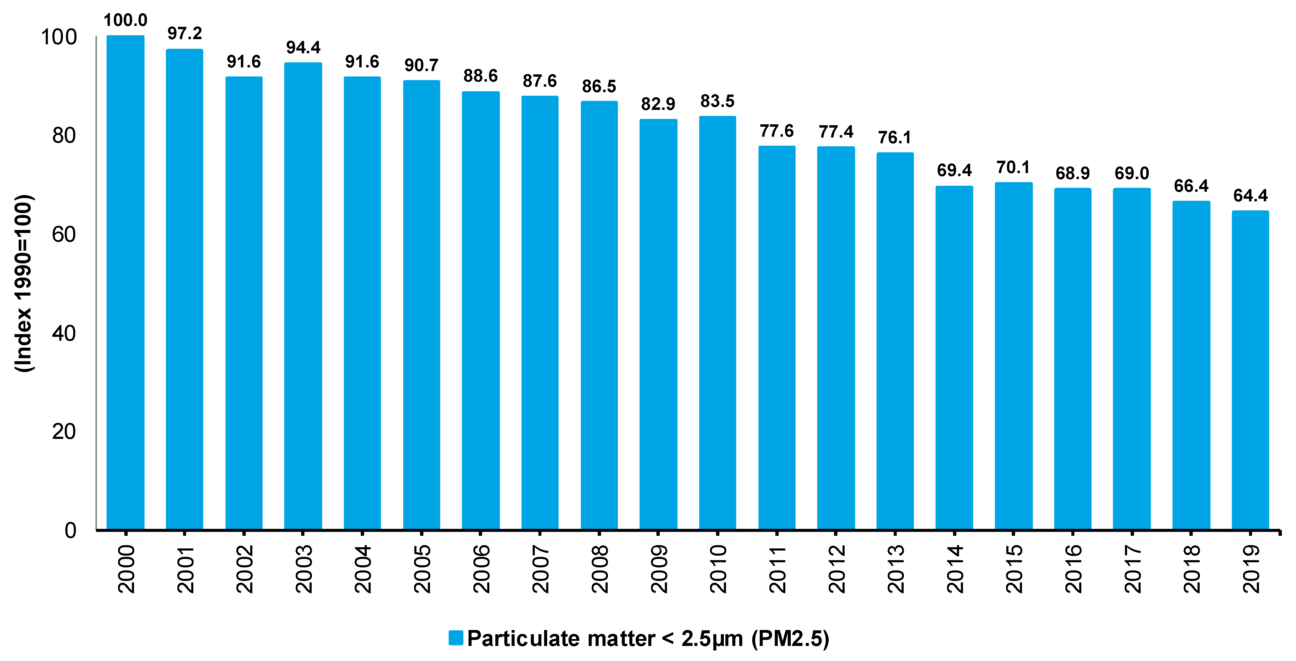
In the EU, the PM2.5 emissions have decreased to about two-thirds of their 2000 levels (as shown in Figure 2). The timeline of emissions reductions shows that the EU-27 as a whole is on track to achieve the reduction target set by the National Emission Ceilings Directive (NECD). Moreover, the NECD set emission ceilings for 2010 and for PM2.5 emissions and emissions reduction commitments for 2020 and 2030.

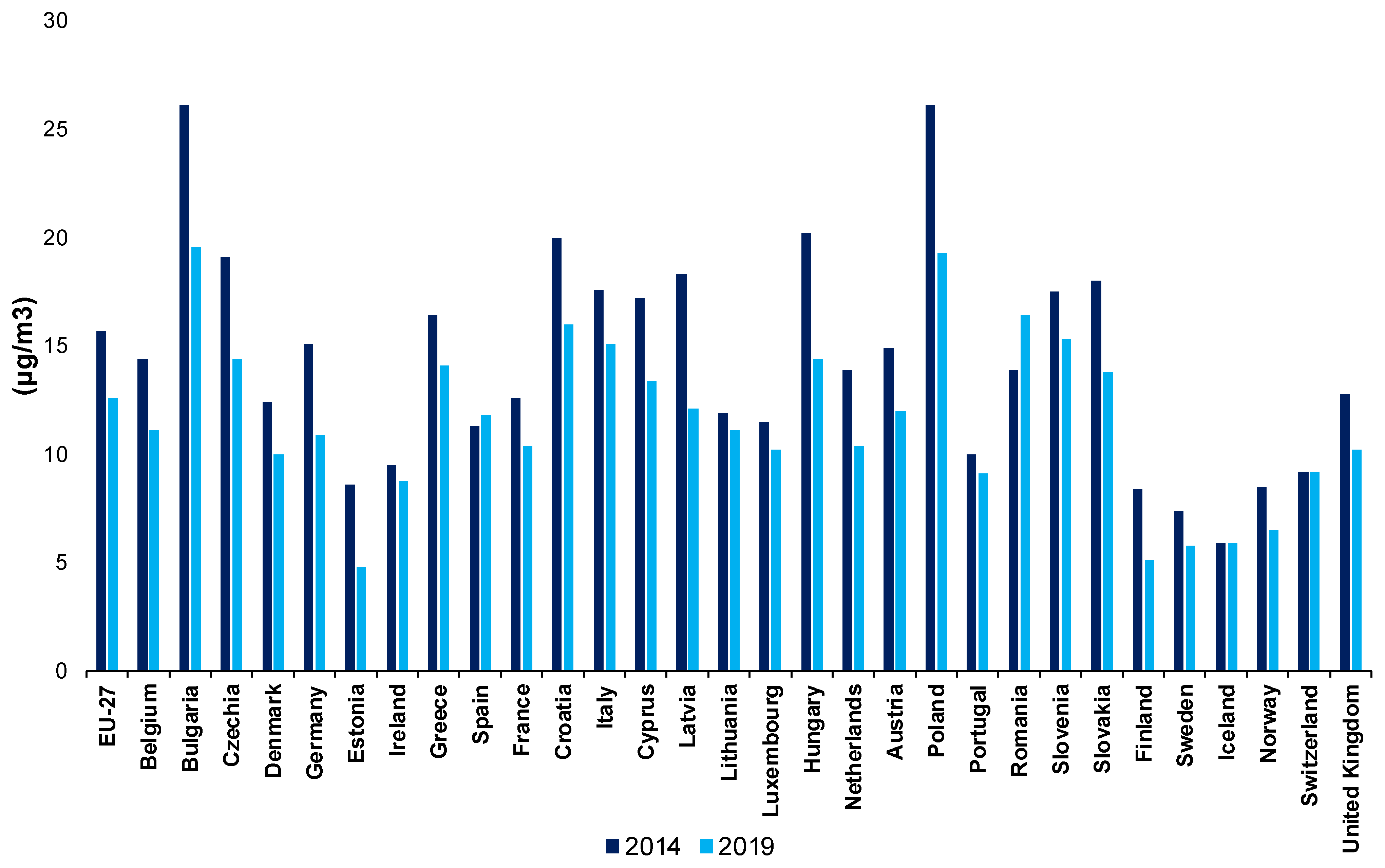
Therefore, in 2000 the PM2.5 emissions were 1,726,970 Gg (1000 tonnes) and in 2019 reached a value of 1,111,440 Gg (1000 tonnes). That is a reduction to about two-thirds (64.4%) of 2000 levels between 2000–2019. The country-specific PM2.5 timelines suggest that four countries (Bulgaria, Poland, Romania, and Croatia) cannot meet their commitments by 2020 (as shown in Figure 3).

As exposed in Figure 3, the annual mean concentration of PM2.5 is highest in 2019 in the urban areas of Bulgaria (19.6 μg/m³) and Poland (19.3 μg/m³), followed by Romania (16.4 μg/m³) and Croatia (16 μg/m³). Therefore, these countries may need to implement emission reduction measures beyond those currently in place. In contrast, the average value for the EU-27 is 12.6 μg/m³, and in some countries of the EU, the concentration of PM2.5 is lowest in urban areas. This is the case in Estonia (4.8 μg/m³), Finland (5.1 μg/m³), and Sweden (5.8 μg/m³). In these countries, the mean of PM2.5 air pollution in 2019 continued with high levels, that were above the WHO recommended levels. Although this type of air pollution has for several years been below the limit set for 2015 (25 μg/m³ annual average), substantial air pollution hotspots remain. Additionally, despite a gradual decrease in recent years, air pollution levels in 2019 remain above the WHO recommended level (10 μg/m³ annual average).

These emissions in the EU come from the commercial, institutional, and households’ sector (55.49%), industrial processes and product use sector (11.98%), road transport sector (10.67%), energy use in the industry sector (8.15%), energy production and distribution sector (3.87%), waste sector (3.80%), no-road transport sector (2.69%), agriculture sector (3.31%), and other (0.04%) (as shown in Figure 4).

The contribution of 11% from the road transport sector indicates that current transport systems based on conventional vehicles are unsustainable from an environmental, health, social, and economic perspective [7]. Indeed, from a health perspective, the increase of PM2.5 emissions caused by vehicular emissions has adverse health effects and may cause premature deaths. Moreover, according to Thunis et al. [1], exposure to PM2.5 is responsible for an average loss of life of about 8 to 10 months in the most polluted regions and cities of the EU. Therefore, electric vehicles, which include battery electric vehicles (BEVs) and plug-in hybrid electric vehicles (PHEVs), are widely considered as a solution to many of the negative impacts of their conventional counterparts [7]. Furthermore, given their potential to reduce local air pollution and greenhouse gas emissions, consumers, businesses, and governments increasingly support electric vehicles [8].

The main objective of this research is to identify the effect of electric vehicles (e.g., BEVs and PHEVs) on PM2.5 in European countries. As we already know, BEVs are purely electric vehicles that exclusively use chemical energy stored in rechargeable batteries, with no secondary source of propulsion. Therefore, this type of vehicle does not emit exhaust emissions. Furthermore, the adoption of these vehicles is generally seen as a highly effective measure to improve air quality [7]. PHEVs are hybrid electric vehicles whose battery can be recharged by connecting a charging cable to an external electrical power source and internally by the onboard generator an internal combustion engine. They emit exhaust emissions in a reduced form when compared to internal combustion engine vehicles (ICEVs) [7].

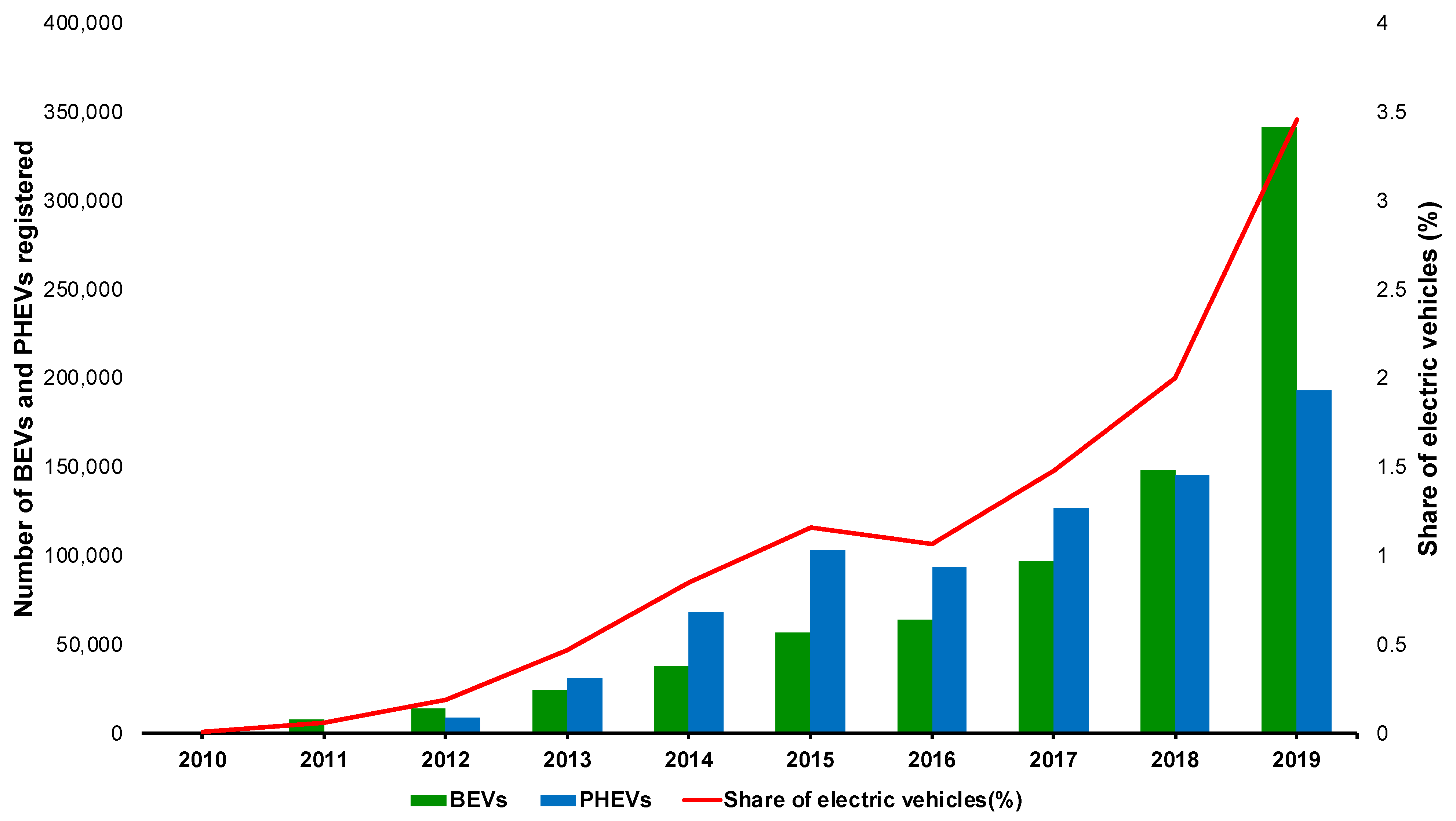
In the European region, BEVs and PHEVs are gradually penetrating the market. However, despite a steady increase in the number of new electric vehicle registrations (BEVs and PHEVs) annually, from 734 units in 2010 to around 534,583 units in 2019, they still represent a market share of only 3.5% of newly registered passenger vehicles. BEVs accounted for 2.2% of all newly registered vehicles in 2019, representing about two-thirds of electric car sales, while PHEVs accounted for 1.3% (as shown in Figure 5).

As shown in Figure 5, the number of new electric cars registered in the EU is increasing. In fact, more than half of these registrations were made in Germany, Norway, the Netherlands, France, and the United Kingdom (e.g., EEA [9]). Indeed, in some countries in Europe (e.g., Cyprus, Estonia, Greece, Lithuania, Slovakia, and Slovenia), the number of BEVs in the total number of registered vehicles remained below 200 units in 2019. However, between 2018 and 2019, a notable increase (129%) in new registrations was registered. This increase can be partly explained by the inclusion of Norway in the dataset in 2019, a country that registered about 60,000 electric cars [9]. In fact, regarding the total number of electric vehicles in the fleet, the number of BEVs in 2010 was 734, and in 2020 reached 720,913. The total number of PHEVs was 9000 in 2012 and reached a value of 603,314 in 2020. Germany, Norway, the United Kingdom, France, and the Netherlands are the top 5 countries with a significant number of BEVs and PHEVs in the EU in 2020, while Liechtenstein, Cyprus, and Latvia are countries with fewer BEVs and PHEVs in the fleet in the region [9].

Furthermore, in Germany, the number of registered BEVs in the fleet was 308,139, while the number of PHEVs was 287,037 in 2020. In Norway, the number of registered BEVs in the fleet was 319,540 and PHEVs was 134,420. In the United Kingdom, the number of registered BEVs in the fleet was 206,998 and PHEVs was 240,631. In France, the number of registered BEVs in the fleet was 277,001 and PHEVs was 132,309. Furthermore, in the Netherlands, the number of registered BEVs in the fleet was 172,534 and PHEVs was 100,371 [9].

Although increasing the market share of BEVs and PHEVs could help the EU meet its emission reduction targets and ensure progress towards its long-term climate neutral strategy by 2050, their implications for PM2.5 emissions remain less understood. This vision is shared by Requia et al. [8]. The authors assessed 4734 studies on the impact of a shift to greater electric car (BEVs and PHEVs) use. Of the 65 studies that fulfilled the inclusion criteria for the review, the authors concluded that while the benefits of electric cars concerning the exhaust emissions of several air pollutants are well-established, less evidence exists regarding the impact of electric car use on PM2.5 emissions.

As mentioned above, few studies exist that analyse the effect of BEVs and PHEVs on PM2.5 emissions. Most of them are related to and studied by the field of engineering. Studies of this topic do not relate to macroeconomics or use econometrics. This scarcity allows us to conclude that a gap exists in economic theory on the impact of electric vehicles on PM2.5 emissions.

Of the few studies in technologies and engineering, most have shown that electric vehicles improve the environment and reduce PM2.5 emissions, CO₂ emissions, and greenhouse emissions by assessing the life cycle of electric cars, with a particular focus on BEVs and PHEVs (e.g., Rangaraju et al. [10]; Timmers and Achten [11]; Alam et al. [12]; Vilchez et al. [13]; Xiong et al. [14]; Ajanovic and Haas [15]; Wang et al. [16]; Vilchez and Jochem [17]; Wang et al. [18]; Andersson and Börjesson [19]; Zhao et al. [20]; and Ma et al. [21]).

Faced with a lack of literature that addresses the effect of electric vehicles (e.g., BEVs and PHEVs) on PM2.5 emissions in European countries using a macroeconomic and econometric approach, this investigation elaborates on the following central question: Can BEVs and PHEVs mitigate the PM2.5 emissions in European countries? To answer this central question, an empirical analysis was performed. This analysis was based on the macroeconomic panel data of 29 European countries between 2010 and 2019. Moreover, the method of moments quantile regression (MM-QR) and ordinary least squares (OLS) with fixed effects will be used.

This empirical investigation is innovative and will contribute to the literature for several reasons. First, by introducing a new analysis related to the effect of electric vehicles on PM2.5 emissions in the European countries. Moreover, economists do not usually investigate this issue, and this study can open new opportunities for study related to this topic using an econometric and macroeconomic approach. Therefore, this makes our study innovative when compared with others. Second, this investigation will introduce new econometric models to this topic of investigation (e.g., MM-QR and OLS with fixed effects). It can also be considered innovative because of the use of a new econometric approach on a new case study. Finally, this investigation will support policymakers in developing consistent initiatives that promote the development and commercialisation of electric vehicles in European countries. Moreover, it will also help to create more policies to reduce the consumption of fossil fuels to mitigate environmental degradation.

This investigation is divided into seven sections, as follows: Section 2 will present the literature review; Section 3 will present the data and methods; Section 4 will present the empirical results; Section 5 will present the discussions of the results that were found; Section 6 will present the conclusions and policy implications; and Section 7 will present the limitations of this study.

2. Literature Review

This section is divided into two main subsections. Section 2.1 examines the studies conducted on the effects of electric vehicles on the PM2.5 emissions, and Section 2.2 examines the effects of GDP per capita, urbanisation, energy intensity, and fossil energy consumption on PM2.5 emissions.

2.1. The Effect of Electric Vehicles on PM2.5 Emissions

Wang et al. [18] investigated if electric cars could significantly reduce PM2.5 and NO₂ emissions throughout China. The results showed that the use of electric vehicles reduces PM2.5 emissions by 30–70% and NO₂ by 30–80% in most parts of China. Rangaraju et al. [10] investigated the effects of power composition, charge characteristics, and driving behaviour of battery-powered electric vehicles (BEVs) on the emissions performance of CO₂, SO₂, NO_x, and PM2.5 in Belgium. The results showed that CO₂, SO₂, NO_x, and PM2.5 emissions in the reservoir per kilometre are significantly reduced when the BEVs are charged during off-peak hours instead of peak hours. Wang et al. [16] studied the uncoordinated emission reduction mechanism (e.g., CO₂, NO_x, SO₂, and PM2.5). The results showed that a reduction of 78% of CO₂, 94% of NO_x, 98% of SO₂, and 99% of PM2.5 is possible. A sensitivity analysis showed that upgrading electric vehicles could reduce local emissions of CO₂, NO_x, SO₂, and PM2.5 in Beijing. Vilchez et al. [13] modelled the effects of EU electric vehicle designs on emissions (CO₂ and PM2.5) with three models (PRIMES-TREMOVE, DIONE, and SHERPA). The results indicated that electric vehicles led to a 3% decrease in PM2.5.

Timmers and Achten [11] investigated the emission of non-exhaust PM2.5 from electric vehicles. The results showed that vehicle weight affects non-exhaust PM2.5 emissions. Electric cars are 24% heavier than similar non-electric models. According to available data, PM1.0 emissions in electric vehicles are about the same average of conventional cars. Electric cars emit slightly less PM2.5, averaging 1% to 3% less than ICEVs emitted by benzene combustion engines. Alam et al. [12] analysed the effects of passenger cars on reducing PM2.5 and CO₂ emissions using a two-scenario approach (Electric Vehicle Policy Scenario and Normal Car Sales Ban Scenario by 2030) in Ireland during the period from 2015–2035. The results showed that CO₂ emissions were continuously reduced during the forecast period. However, the decline in PM2.5 from 2028 forward was reversed due to the non-exhaust increase in PM2.5 emissions. Under two alternative scenarios, a 52% to 69% reduction in CO₂ is possible, while only a 9% to 15% reduction in PM2.5 by 2035 is achievable. Ma et al. [21] investigated the impact of electric vehicle policies on the environment in the Beijing-Tianjin-Hebei District under two scenarios. The results showed that under the electric vehicle policy (REN) scenario, PM2.5 emissions will decrease by 18.84%, 20.04% and 19.57% by 2030 in Beijing, Tianjin, and Hebei, respectively. However, under the scenario without electric vehicle policies (FOS), the PM2.5 concentration decreases by 11.38%, 15.12%, and 22.27%, respectively.

2.2. The Effect of Other Variables (Control Variables) on PM2.5 Emissions

Some studies showed that GDP per capita positively impacts PM2.5 emissions (e.g., Li et al. [22]; Ma et al. [23]; Hao and Liu [24]; Cheng et al. [25]; Xu and Lin [26]; Wu et al. [27]; Zhao et al. [28]; Chen et al. [29]; Wang et al. [30]; Yang et al. [31]; and Xie and Sun [32]), while many other studies have shown this effect to be negative (e.g., Wu et al. [27]; Wang et al. [33]; Wang et al. [34]; Zhang et al. [35]; and Zhu et al. [36]). On the other hand, the effects of urbanisation on PM2.5 concentrations have indicated mixed results. Some studies have shown this effect to be positive (e.g., Li et al. [22]; Ma et al. [23]; Chen et al. [29]; Zhao et al. [28]; Wang et al. [33]; Wang et al. [34]; Zhu et al. [36]; Yan et al. [37]; and Zou and Shi [38]). Several other studies have shown that urbanisation has negative effects on PM2.5 emissions (e.g., Xu and Lin [26] and Zhang et al. [35]). Finally, regarding the impact of energy intensity and fossil energy consumption, the results of most studies showed that the effects of these two variables increase the PM2.5 emissions (e.g., Cheng et al. [25]; Xu and Lin, [26]; Wu et al. [27]; Zhao et al. [28]; Chen et al. [29]; Yang et al. [31]; Xie and Sun [32]; Wang et al. [34]; Zhang et al. [35]; Zou and Shi [38]; and Soleimani et al. [39]).

Yang et al. [31] investigated the socioeconomic effects of PM2.5 emissions in Chinese cities using spatial econometrics from 2006–2016. The results showed that energy intensity and economic growth increase PM2.5 emissions. Li et al. [22] examined for China, from 1999–2011, the effect of economic growth, urbanisation, and industrialisation on PM2.5 emissions. The results showed that economic growth, urbanisation, and industrialisation are associated with increased PM2.5 emissions. Finally, Wu et al. [27] studied the relationship between urbanisation and PM2.5 concentration in four regions (e.g., China, East China, Middle China, and West China). The results showed that economic growth in China and East China has a negative effect on PM2.5 emissions and an N-inverse relationship with it. In contrast, in middle China and West China, it positively impacts PM2.5 concentration.

Furthermore, this relationship in middle China and west China is U-Inverted and linear, respectively. At the same time, energy consumption increases the PM2.5 emissions in all regions. Xu and Lin [26] investigated the cause of significant regional differences in PM2.5 emissions in China using the quantile regression model. The results showed that economic growth, energy intensity, and energy consumption structure positively and significantly affect the PM2.5 emissions, more significantly in higher quantiles. In comparison, urbanisation has a negative and significant impact on PM2.5 concentration. Yang et al. [31] investigated the socioeconomic effects on PM2.5 emissions in Chinese cities using spatial econometrics from 2006 to 2016. The results showed that energy intensity and economic growth increase PM2.5 emissions.

Hao and Liu [24] examined the factors affecting the PM2.5 emissions in 73 cities in China in 2013 using spatial econometric analysis. The results showed that GDP per capita has a U-shaped inverse relationship to PM2.5. In addition, the number of vehicles has a significant positive effect on the urban PM2.5 concentration. Ma et al. [23] analysed the impact of regional economic activities on PM2.5 pollution in 152 Chinese cities using a spatial autoregression model. The results showed that urbanisation, GDP, energy intensity, and the number of cars positively affected PM2.5 pollution. Wang et al. [30] examined the deregulation reform on PM2.5 emissions in 283 Chinese cities from 2000–2013. The results indicated a correlation between the Kuznets GDP per capita and PM2.5 concentration in China. Zhao et al. [28] investigated the effects of economic development, energy consumption, urbanisation, industrialisation, and the number of vehicles on Chinese PM2.5 concentrations from 1998 to 2016 using an ARDL model. The results indicated an inverse relationship between PM2.5 concentration and GDP per capita. The results also showed that energy consumption and urbanisation positively affect PM2.5 emissions. Cheng et al. [25] identified the spatial effects and triggers of PM2.5 pollution in 285 cities in China using the dynamic space panel model from 2001–2012. The results showed an inverse U-shaped relationship between GDP per capita and PM2.5 emissions. Also, energy intensity increases the PM2.5 concentration. Xie and Sun [32] investigated the effect of FDI on PM2.5 concentration in emerging countries using the generalised panel smooth transition regression (GPSTR) model during the period from 2010–2016. The results showed an N-shaped relationship between GDP per capita and PM2.5 concentration, and energy intensity increases PM2.5 emissions.

Chen et al. [29] examined the effect of energy consumption structure, economic growth, energy intensity, and urbanisation on PM2.5 concentrations in countries worldwide from 1998–2014. The results showed that energy consumption, energy intensity, economic growth, and urbanisation lead to an increase in PM2.5 concentrations in the long run. Wang et al. [33] examined the emission factors of PM2.5 in 190 Chinese cities in 2014. The results indicated that urbanisation was positively correlated with PM2.5 emissions, while GDP per capita was negatively correlated with PM2.5 concentrations. Wang et al. [34] addressed the heterogeneous effects of democracy, political globalisation, and urbanisation on PM2.5 concentrations in G20 countries. The results showed that economic growth has a negative impact on PM2.5 emissions and that this relationship is U-shaped.

In contrast, fossil energy consumption and urbanisation have a positive relationship with the release of PM2.5. Zhang et al. [35] examined socioeconomic factors and regional differences in PM2.5 emissions in 225 Chinese cities in 2015. The results showed that urbanisation and economic development have a negative and significant relationship with PM2.5 emissions, while energy intensity increases the PM2.5 concentration.

Zhu et al. [36] investigated the effects of urbanisation on PM2.5 concentration in Yangtze, China, using a spatial econometric model from 2003–2014. The results showed that urbanisation has a positive and significant effect on PM2.5 concentration, while GDP per capita has a negative but negligible effect. Chen et al. [29] examined the impact of energy consumption structure, economic growth, energy intensity, and urbanisation on PM2.5 concentration in countries worldwide from 1998–2014. The results showed that energy consumption, energy intensity, economic growth, and urbanisation lead to an increase in PM2.5 concentration in the long run. Economic growth was the main variable that affected the PM2.5 concentration in the global panel, the high-income panel, and the high-middle-income panel. Using the Bayesian hierarchical spatial regression, Zou and Shi [38] investigated the heterogeneous socioeconomic effects of PM2.5 emissions in 30 regions in China. The results showed that urbanisation has a higher and positive impact in high quantiles, while energy efficiency reduces the PM2.5 emissions. Soleimani et al. [39] identified the source of heavy metals in PM2.5 emissions in Isfahan, Iran, between March 2014 and March 2015. The results indicated that the most important sources of heavy metals are fossil fuel combustion, car tire wear, industrial activities (such as the iron and steel industry), and dust storms.

As can be seen, several studies have been conducted in different countries and regions using different models. The innovation of this research examines the effects of BEVs and PHEVs on PM2.5 emissions in European countries separately using the method of moments quantile regression (MM-QR). The following section introduces research data and methods.

3. Data and Method

As mentioned before, this section will present the data and methods used to carry out this empirical investigation. Therefore, Section 3.1 will present the data/variables that will be used, and Section 3.2 will present the methods.

3.1. Data

In order to carry out this empirical investigation, data were collected from 29 countries from the European region between 2010 and 2019. The European countries that were selected are Austria, Belgium, Bulgaria, Croatia, Cyprus, Czechia, Denmark, Estonia, Finland, France, Germany, Greece, Hungary, Iceland, Ireland, Italy, Latvia, Lithuania, Luxembourg, the Netherlands, Norway, Poland, Portugal, Romania, Slovakia, Slovenia, Spain, Sweden, and the United Kingdom.

These 29 countries were selected because electric vehicles are gradually penetrating the European market. However, the number of new electric vehicle registrations (BEVs and PHEVs) annually, from 734 units in 2010 to about 534,583 units in 2019, still accounts for a market share of only 3.5% of newly registered passenger vehicles. BEVs accounted for 2.2% of total new car registrations in 2019, representing around two-thirds of electric car sales, while PHEVs represented 1.3% [9]. As this investigation will address a macroeconomic aspect, it is convenient to use all countries from the European region. Moreover, this investigation used data from 2010 to 2019 because the OECD data provides data until 2019 for the variable PM2.5, and the EAFO [40] provides data beginning in 2010 for the variables BEVs and PHEVs. Therefore, the variables selected to carry out this empirical investigation will be shown in

Table 1. The variable definitions and sources.

Variable Abbreviation	Variable Definition	Sources
PM2.5	Particulate matter (Micrograms per cubic metre).	OECD DATA [41]
BEVs	The number of battery electric vehicles (BEVs) registered in the fleet (Passager cars).	European Alternative Fuels Observatory (EAFO) [40]
PHEVs	The number of plug-in hybrid electric vehicles (PHEVs) registered in the fleet (Passager cars).	European Alternative Fuels Observatory (EAFO) [40]
EI	Energy intensity (kg of oil equivalent/gdp 2010$).	British Petroleum (BP) [42]
GDP	Gross domestic product (GDP) per capita (constant = 2010$).	World Bank Data (WBD) [43]
URB	Urban population = % of total population.	WBD [43]
FOSSIL	Fossil fuel energy consumption (e.g., oil, gas, and coal) kg of oil per capita.	WBD [43]

Notes: all data are annual from 2010 to 2019.

. Indeed, this table shows the variable definitions and the sources of variables.

This investigation will use the following variables: PM2.5, BEVs, PHEVs, EI, GDP, URB, and FOSSIL. PM2.5 is our dependent variable, while BEVs, PHEVs, EI, GDP, URB, and FOSSIL are our independent variables. Moreover, EI, GDP, URB, and FOSSIL are the control variables. Therefore, after presenting the variables, it is also necessary to present the methods used in this empirical investigation.

3.2. Methods

As mentioned before, this subsection presents the methods used in this empirical investigation. Therefore, this subsection will present the MM-QR and OLS with fixed effects models and the preliminary tests.

3.2.1. MM-QR Model

This study adopted the MM-QR approach for panel fixed effects as the main method to explore the impact of electric vehicles on PM2.5 emissions in European countries. Machado and Silva [44] developed this model. Moreover, according to Usman et al. [45], this method can capture the unobserved distributional heterogeneity across countries within a panel. Fuinhas et al. [46] point out that the MM-QR method has other advantages. According to the authors, this method assumes that the covariate affects only the variables of interest through the location channel. Moreover, the same authors state that this method also assumes that the covariate affects only the variables of interest through the scale functions relative to a mere shifting. Moreover, this method can examine the conditional heterogenous covariance effects of the determinants of PM2.5 emissions at different quantiles [44].

The typical definition of MM-QR can be presented as the following (Equation (1)):

$$Q_{PM2.5}\left(\tau |X_{it}\right)=\left({\alpha }_i+{\delta }_{i}q\left(\tau \right)\right)+y_{it}^{’}\beta +Z_{it}^{’}\gamma q\left(\tau \right)$$

(1)

where the scalar coefficient ${\alpha }_i\left(\tau \right)={\alpha }_i+{\delta }_{i}q\left(\tau \right)$ denotes the quantile- $\tau$ fixed effects for an individual country. The distributional impact varies from the classical fixed effect, given that it is not location fixed [46]. Moreover, Machado and Silva [44] state that the distribution impact depicts the time-invariant traits that allow other variables to have diverse effects on investigated countries.

3.2.2. OLS with Fixed Effects Model

According to Fuinhas et al. [46], the OLS with fixed effects can estimate the slope and intercepts for a set of observations. Moreover, the same authors state that this model can estimate the mean response for the fixed predictors (see Equation (2)).

LPM2.5_it = β₀ + β₁LGDP_it + β₂LBEVs_it + β₃LPHEVs_it + β₄LEI_it + β₅LURB_it + β₆LFOSSIL_it + ε_it

(2)

where β₀ is the intercept and β is the value of fixed covariates being fitted to predict the dependent variable LPM2.5_it, ε_i is the error term, and each variable enters regression for country i at year t.

Indeed, before realising model estimations, it is necessary to carry out the preliminary tests. Therefore, the following subsection will illustrate the initial tests used in this empirical analysis.

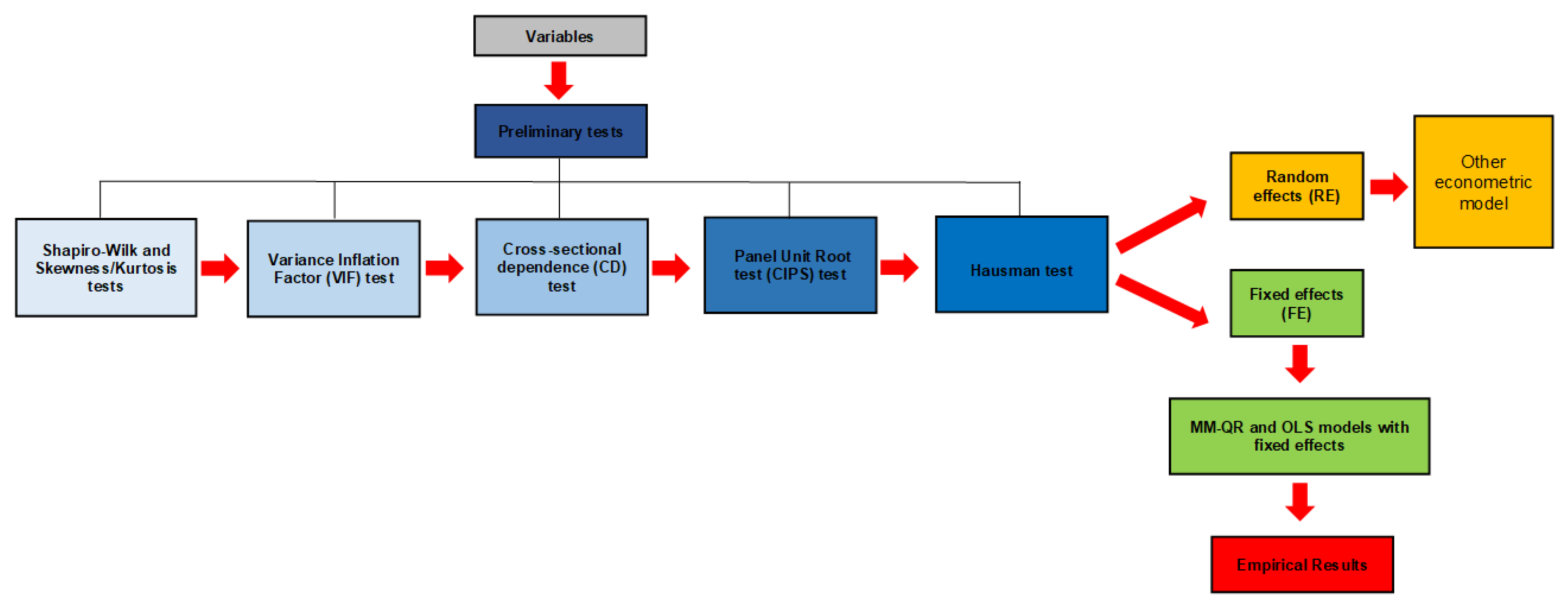
3.2.3. Preliminary Tests

The preliminary tests need to be carried out before the MM-QR and OLS model estimations. The preliminary tests are necessary to identify the characteristics of variables and the existence of singularities. Indeed, a lack of preliminary tests could lead to inconsistent and improper interpretations [47]. Therefore, the following tests will be done:

(I) 

Shapiro-Wilk [48]. This test checks the presence of normality in the panel model;

(II) 

Skewness/Kurtosis [49]. This test checks the presence of normality in the panel model;

(III) 

Variance Inflation Factor (VIF) [50]. This test identifies the presence of multicollinearity between the variables of the model;

(IV) 

Cross-sectional dependence (CD) [51]. This test checks the presence of cross-sectional dependence in the variables of the model;

(V) 

Panel Unit Root test (CIPS) [52]. This test verifies the presence of unit roots in the variables;

(VI) 

Hausman [53]. This test verifies the random effects vs fixed effects and identifies heterogeneity.

Therefore, this investigation will follow the following conceptual framework, highlighting the methodological approach used (as shown in Figure 6).

The econometric software Stata 17.0 was used to carry out this empirical investigation. Moreover, the Stata commands, such as sum, sktest, swilk, vif, xtcd, multipurt, hausman, xtqreg, and xtreg will be used to realise the preliminary tests and model estimations. The following section will present the empirical results of this study.

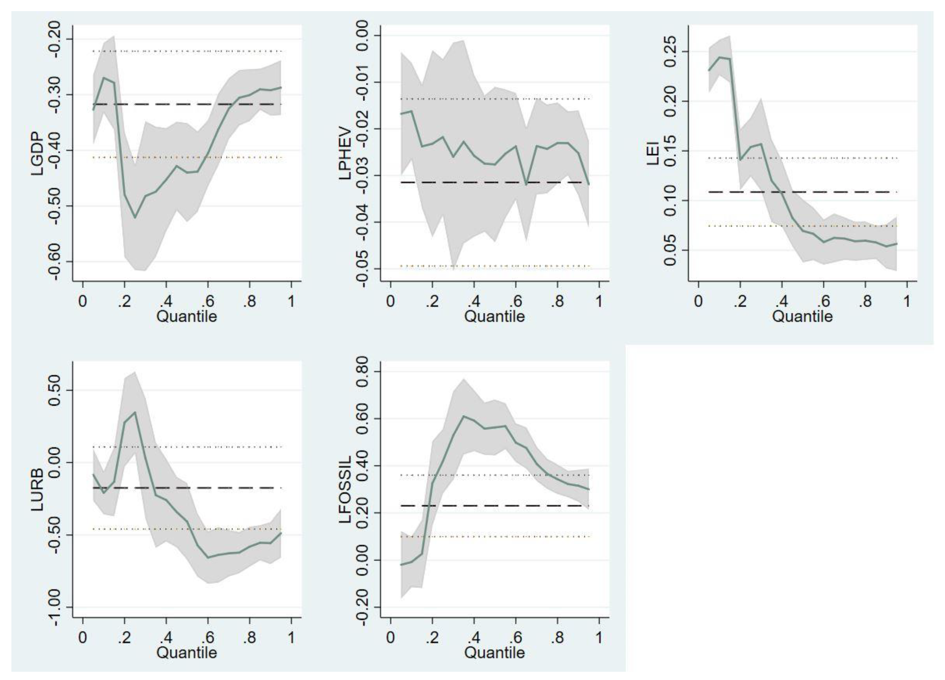
4. Empirical Results

The experimental results section consists of two subsections: the variables’ statistical characteristics and preliminary tests are given in the first subsection. The MM-QR results are shown in the second subsection.

4.1. Preliminary Tests

Before performing the preliminary tests, we reviewed the statistical data characteristics.

Table 2. The descriptive statistics.

Variables	Descriptive Statistics
	Obs.	Mean	Std. Dev.	Min.	Max.
LPM2.5	290	13.3991	5.1657	5.3344	27.3647
LGDP	290	73,528.62	46,612.05	13,989.86	219,770.61
LBEVs	290	3244.638	9008.5	0	61,544
LPHEVs	290	2753.779	7346.283	0	44,795
LEI	290	0.5759	0.6475	0.0162	2.5015
LURB	290	73.3393	12.5514	52.6582	98.0414
LFOSSIL	290	2663.4	1194.5	1195.3	8270.6

Notes: Obs. is the number of observations in the model, Std. Dev. is the standard deviation, and Min and Max are the minimum and maximum, respectively.

shows the number of observations, median, standard deviation, minimum and maximum. The number of observations of this research is 290, and the panel is balanced. Moreover, “L” denotes variables in the natural logarithms. Indeed, this investigation transformed all variables in natural logarithms in order to linearise the relationships between model variables (e.g., [46,47]).

After evaluating the statistical characteristics, the normality of the data should be examined, because one of the main conditions for using the MM-QR is abnormal data distribution. In the case of normal distribution, the MM-QR estimation results at different quantile levels are the same as the OLS panel with fixed effects estimation results. For this purpose, the Shapiro-Wilk [54] and Shapiro-France [55] tests were used to evaluate the normality of the variables. The null hypothesis of these two tests is the normal data distribution. As shown in

Table 3. The normal distribution test.

Variables	Shapiro-Wilk Test	Shapiro-Francia Test	Obs.
	Statistic	Statistic
LPM2.5	0.9560 ***	0.9591 ***	290
LGDP	0.9696 ***	0.9722 ***	290
LBEVs	0.9892 ***	0.9921 ***	290
LPHEVs	0.9765 ***	0.9848 ***	290
LEI	0.9639 ***	0.9671 ***	290
LURB	0.9579 ***	0.9616 ***	290
LFOSSIL	0.9594 ***	0.9604 ***	290

Notes: *** denotes statistical significance at the 1% level; Obs. is the number of observations.

, all variables reject the null hypothesis, which indicates an abnormal data distribution, so MM-QR can be used to estimate.

After examining the normality test and confirming the abnormal distribution of the data, multicollinearity between the model variables should be examined in the next step. The variance inflation factor (VIF) test was used for this purpose [50]. In this study, the impact of BEVs and PHEVs on PM2.5 emissions has been investigated separately.

Table 4. The VIF test.

Variables	VIF-Test (BEVs)		Variables	VIF-Test (PHEVs)
	VIF	Mean VIF		VIF	Mean VIF
LPM2.5	N.A.	1.89	LPM2.5	N.A	1.84
LGDP	2.83		LGDP	2.56
LBEVs	1.81		LPHEVs	1.79
LEI	1.40		LEI	1.37
LURB	1.73		LURB	1.76
LFOSSIL	1.69		LFOSSIL	1.70

Notes: N.A. denotes not available.

shows the results from the VIF test in both models.

The results from Table 4 showed that since the value of VIF for the variables of both models is less than the 10 benchmarks. Also, the average VIF for both models is less than the normal average of 6. Therefore, the multicollinearity results in these two models do not pose a particular problem [56]. After examining the multicollinearity test, the cross-sectional dependency test of the data panel is examined to evaluate the existence of common characteristics and shocks in countries [47]. A Pesaran CD-test was used in this study [51]. The null hypothesis is the absence of cross-sectional dependence. As shown in

Table 5. The Pesaran CD-test.

Variables	CD-Test	p-Value
LPM2.5	44.43	0.000 ***
LGDP	51.13	0.000 ***
LBEVs	40.61	0.000 ***
LPHEVs	43.38	0.000 ***
LEI	44.83	0.000 ***
LURB	36.86	0.000 ***
LFOSSIL	27.35	0.000 ***

Notes: *** denotes statistical significance at the 1% level.

, the null hypothesis is rejected for all variables, indicating a cross-sectional dependency between all of them.

After confirming the existence of cross-sectional dependence, the next step is to examine the panel data unit root tests. In this research, the CIPS-test provided by Pesaran [52] has been used. As shown in

Table 6. The unit root test.

Variables	Panel Unit Root Test (CIPS) (Zt-Bar)
	Without Trend		With Trend
	Lags	Adjusted t	Adjusted t
LPM2.5	1	−5.458 ***	−2.200 **
LGDP	1	−4.320 ***	−3.054 ***
LBEVs	1	−0.979	−1.353 *
LPHEVs	1	−4.791 ***	−4.154 ***
LEI	1	−1.083	−3.758 ***
LURB	1	−2.238 **	−1.791 **
LFOSSIL	1	−0.459	−3.866 ***

Notes: ***, **, * denotes statistical significance at the 1%, 5%, and 10% levels, respectively.

, the variables LPM2.5, LGDP, LPHEVs, and LURB are without and with a trend stationary. At the same time, the variables LBEVs, LEI, and LFOSSIL are only stationary with the trend.

Before performing the MM-QR and OLS with fixed effects models, the existence of fixed effects (FE) or random effects (FE) of the model should be checked using the Hausman test. The null hypothesis indicates the absence of systematic differences in coefficients and confirms the existence of random effects (RE). In contrast, the rejection of the null hypothesis suggests a model with fixed effects (FE). Therefore, the Hausman test is performed for two models, as shown in

Table 7. The Hausman test.

Model	Prob > chi2(3)
Model I—BEVs vs LPM2.5	0.1487 **
Model II—PHEVs vs LPM2.5	0.1931 **

Notes: ** denotes statistical significance at the 5% level.

; both models reject the null hypothesis, representing the two models with fixed effects.

After confirming both models with fixed effects, the serial correlation is evaluated. The Bias-corrected LM-based test presented by [57] was used in this study. The null hypothesis is the absence of autocorrelation to the second order.

Table 8. The Bias-corrected LM-based test.

Variables	LM(k)-Stat	p-Value	Balanced?
LPM2.5	74.56	0.0000 ***	Balanced
LGDP	25.67	0.0000 ***	Balanced
LEI	23.00	0.0000 ***	Balanced
LURB	21.16	0.0000 ***	Balanced
LFOSSIL	52.83	0.0000 ***	Balanced
LBEVs	11.53	0.0000 ***	Balanced
LogPHEV	10.14	0.0000 ***	Balanced

Notes: *** denotes statistical significance at the 1% level.

shows that the null hypothesis cannot be rejected.

Moreover, the results found in this test also confirm that the panel data used in this study is balanced. The following section will show evidence of the results from the MM-QR and the OLS with fixed effects.

4.2. MM-QR Results

After performing the preliminary tests, we estimate the MM-QR and OLS with fixed effects for both models. Before estimating the models, we divide the countries into six groups according to the average PM2.5 emissions from 2010 to 2019 (

Table 9. The country distribution of PM2.5 emissions.

Quantile	Country
The lower 10th ($0\le quantile<10$)	Iceland, Sweden, and Finland
The 10–25th ($10\le quantile<25$)	Ireland, Norway, Estonia, and Austria
The 25–50th ($25\le quantile<50$)	France, Lithuania, Luxembourg, the United Kingdom, Denmark, Spain, and Portugal
The 50–75th ($50\le quantile<75$)	Romania, Cyprus, Greece, Latvia, Belgium, Germany, and the Netherlands
The 75–90th ($75\le quantile<90$)	Croatia, Czechia, Slovenia, Hungary, and Italy
The upper 90th ($quantile\ge 90$)	Poland, Bulgaria, and Slovakia

Notes: According to the level of PM2.5, we divided the panel of 29 countries into six grades.

). Then we estimate the MM-QR based on the 10th, 25th, 50th, 75th, and 90th quantiles.

Table 10. The estimation results from the panel quantile regression model and panel fixed effects (Model I).

	Dependent Variable: LPM2.5
Independent Variables	Quantiles					OLS
	10th	25th	50th	75th	90th	Fixed Effects
LGDP	−0.2902 ***	−0.4040 ***	−0.4078 ***	−0.3012 ***	−0.2549 ***	−0.2593 *
LBEVs	−0.0129	−0.0467 **	−0.0332 **	−0.0255 ***	−0.0307 ***	−0.0142 ***
LEI	0.2501 ***	0.1797 ***	0.0799 ***	0.0629 ***	0.0625 ***	0.2317
LURB	−0.2508 *	0.1730	−0.3670 **	−0.5967 ***	−0.5695 ***	−1.8179 ***
LFOSSIL	0.0341	0.4164 ***	0.5510 ***	0.3579 ***	0.2885 ***	0.3195 ***
Constant	6.9032 ***	9.0101 ***	12.2293 ***	10.950 ***	9.9951 ***	5.4169 ***
Pseudo R2	0.2762	0.3116	0.3755	0.4328	0.4763	0.6379

Notes: ***, **, * denote statistical significance at the 1%, 5%, and 10% levels, respectively.

shows the results of Model I, which estimate the impact of BEVs on PM2.5 emissions by MM-QR. In addition, the estimate of OLS with fixed effects is given to evaluate the robustness check of the model results.

As shown in Table 10, the variable LGDP in all quantiles has a negative effect on PM2.5 emissions. As shown in Figure 7 the LGDP is approximately U-shaped in relation to PM2.5 concentration. The variable LBEVs also has a significant negative effect on PM2.5 emissions in all quantiles except the 10th, and this effect is more significant in the 25th and 50th quantiles. The variable LURB has a negative impact on PM2.5 in other quantiles except for the 25th. As can be seen, this effect is more significant in the 75th and 90th quantiles.

On the other hand, the variables LEI and LFOSSIL positively impact the PM2.5 emissions. As shown in Figure 7, the variable LFOSSIL has a U-inverse relation to PM2.5 emissions. Furthermore, it has the most significant impact on the 50th quantile. As the OLS with fixed effects results in Model I show, the variables LGDP, LBEVs, and LURB have an adverse impact on PM2.5 concentrations, while the variable LFOSSIL increases the PM2.5 emissions. This result confirms the MM-QR. The vertical axis shows the elasticities of the explanatory variables, and the horizontal lines depict the conventional 95% confidence intervals for the OLS coefficient.

After estimating Model I, this investigation will examine the results of estimating Model II, which examines the impact of PHEVs on PM2.5 emissions using the MM-QR and OLS with fixed effects.

According to

Table 11. The estimation results from panel quantile regression model and panel fixed effects (Model II).

Dependent Variable: LPM2.5
Independent Variables	Quantiles					OLS
	10th	25th	50th	75th	90th	Fixed Effects
LGDP	−0.2698 ***	−0.5206 ***	−0.4409 ***	−0.3054 ***	−0.2919 ***	−0.0765
LPHEVs	−0.0162 **	−0.0218	−0.0276 **	−0.0243 ***	−0.0252 ***	−0.0174 ***
LEI	0.2441 ***	0.1539 ***	0.0694 ***	0.0589 ***	0.0538 ***	0.3144 **
LURB	−0.2098 *	0.3462	−0.4074 **	−0.6218 ***	−0.5561 ***	−1.1161 **
LFOSSIL	0.0077	0.4189 **	0.5628 ***	0.3657 ***	0.3151 ***	0.1071
Constant	6.2556 ***	9.3707 ***	12.7789 ***	11.1280 ***	10.4395 ***	4.2203 ***
Pseudo R2	0.2891	0.3271	0.3935	0.4556	0.5049	0.6041

Notes: ***, **, * denote statistical significance at the 1%, 5%, and 10% levels, respectively.

, it can be stated that the variable LGDP at all quantile levels has negative and significant effects on PM2.5 emissions. Moreover, as shown in Figure 8, GDP per capita has a U-shaped relationship with PM2.5 emissions. The variables LPHEVs and LURB also negatively affect PM2.5 emissions at other levels except in the 25th quantile. This effect is higher in the 75th quantile with a coefficient of −0.6218 for the variable LURB than in other levels. On the other hand, the variable LEI positively affects PM2.5 emissions at all quantile levels. Finally, the variable LFOSSIL also has a positive and significant impact on PM2.5 emissions in all quantiles, except for the 10th.

Moreover, this effect is more significant in the 50th (0.5628) quantile. As shown in Figure 8, the variable LFOSSIL has a U-inverse relationship with PM2.5 emissions. The results of OLS with fixed effects estimation also show that the variables LPHEVs and LURB have negative effects on PM2.5 emissions, while the variable LEI increases PM2.5 emissions. As can be seen, the results of the OLS with fixed effects estimation confirm the results of the MM-QR. The vertical axis shows the elasticities of the explanatory variables, and the horizontal lines depict the conventional 95% confidence intervals for the OLS coefficient.

Finally, Figure 9 summarises the results of the effects of the variables in both models on the PM2.5 emissions. Therefore, this figure was based on the results in Table 10 and Table 11.

The following section will briefly discuss the results found by the empirical approach.

5. Discussions

As presented in the section above, the variables LGDP, LBEVs, LPHEVs, and LURB negatively impact PM2.5 emissions, while the variables LEI and LFOSSIL have a positive impact. In light of these findings, this investigation produced the following questions: What are the possible explanations for the results found? Several authors found the negative impact of GDP on PM2.5 emissions (e.g., Wu et al. [27]; Wang et al. [33]; Wang et al. [34]; Zhang et al. [35]; and Zhu et al. [36]). According to Wang et al. [33], the negative impact of GDP on PM2.5 emissions could be related to a lower dependence on fossil fuels. This idea also is supported by Wu et al. [27]. However, according to the authors, the lower dependence on fossil fuels for growth is related to an increase in income per capita that allows for the development and accessing of new technologies with high energy efficiency and green energy technologies by industries and households.

Moreover, Wang et al. [34] state that the increase in income allows for technique improvements through the access of new technologies. Therefore, this improvement allows for less input per unit of output or for the adoption of cleaner production technologies. Therefore, the pollution per unit of output decreases. The same authors add that high-income countries pursue policies focused on achieving stringent environmental standards and innovations to create cleaner energy utilisation, thereby decreasing emissions. Therefore, these aspects allow a negative U-shaped relationship between GDP and PM2.5 emissions in developed countries, as found in this investigation (as shown in Figure 8 and Figure 9).

The negative impact of electric vehicles (e.g., BEVs and PHEVs) on PM2.5 emissions were found by several authors (e.g., Rangaraju et al. [10]; Timmers and Achten [11]; Alam et al. [12]; Vilchez et al. [13]; Xiong et al. [14]; Ajanovic and Haas [15]; Wang et al. [16]; Vilchez and Jochem [17]; Wang et al. [18]; Andersson and Börjesson [19]; Zhao et al. [20]; and Ma et al. [21]). According to Ajanovic and Haas [15], electric vehicles (e.g., BEVs and PHEVs) can mitigate environmental degradation. However, this mitigation depends on the form of production and use of electric vehicles. The authors conclude that the capacity of electric vehicles to mitigate environmental degradation depends on renewable electricity use, and Vilchez and Jochem [17] share this idea. According to the authors, electric cars can mitigate air pollution if the vehicles use electricity from green energy sources.

Xiong et al. [14], who studied the Chinese case, agreed with the visions of Vilchez and Jochem [17] and Ajanovic and Haas [15]. According to the authors, electric cars decrease CO₂ emissions by reducing energy consumption. This view that electric vehicles can reduce energy consumption is supported by Fuinhas et al. [46] and the European Environment Agency [9]. They reveal that the energy consumption from electric vehicles decreased from 264 Wh/km to 150 Wh/km. This result is an indication that electric cars have become more efficient. Moreover, Nielsen and Jørgensen [58] predicted that electric cars would consume less energy. According to the authors, the energy consumption from electric vehicles will be 0.10 kWh/km between 2016 and 2030.

The evidence that electric cars consume less energy in the European region was found by Fuinhas et al. [46] and Koengkan et al. [59]. According to Fuinhas et al. [46], electric vehicles reduce the final energy consumption by -0.0154. Therefore, Fuinhas et al. [46] confirm the evidence that electric cars consume less energy, as mentioned by Ajanovic and Haas [15] and Vilchez and Jochem [17]. Indeed, according to the European Environment Agency [9], this reduction is related to the increase in the energy efficiency of vehicles. However, despite the capacity of electric cars (e.g., BEVs and PHEVs) to mitigate PM2.5 emissions, their impact is small. Indeed, this small impact is related to the low share of electric cars on the market, where this kind of vehicle had 3.5% in 2019 in Europe [9].

Several authors found the negative impact of urbanisation on PM2.5 emissions (e.g., Wu et al. [27]; Wang et al. [33]; Wang et al. [34]; Zhang et al. [35]; and Zhu et al. [36]). Wang et al. [34] point out that the negative impact of urbanisation on PM2.5 emissions could result from the rapid urbanisation process transforming the economies. Urbanisation results in remarkable improvements in urban infrastructure and software facilities. These attract talent to gather in urban areas, contributing to human capital accumulation. Human capital accumulation enhances environmental awareness and promotes the R&D of energy-saving and abatement technologies. Therefore, PM2.5 pollution intensity gradually decreases as the levels of urbanisation increase. The same authors complement that the urbanisation development provides the opportunity for investing in information-based industries and services.

Furthermore, it also improves production techniques or adopts cleaner technology. These impacts are called the composition and technique effects, and they can surpass the scale effect and produce a downward trend in the EKC curve. Other authors share this point of view (e.g., Wu et al. [27]; Wang et al. [33]; Zhang et al. [35]; and Zhu et al. [36]).

Finally, regarding the positive impact of energy intensity and fossil energy consumption on PM2.5 emissions, several authors have found this effect (e.g., Cheng et al. [25]; Xu and Lin [26]; Wu et al. [27]; Zhao et al. [28]; Chen et al. [29]; Yang et al. [31]; Xie and Sun [32]; Wang et al. [34]; Zou and Shi [38]; Soleimani et al. [39]; and Zhang et al. [35]). For Wang et al. [34], the positive impact of energy intensity on PM2.5 emissions is related to the high participation of non-renewable energy on the energy matrix. According to Fuinhas et al. [46], in 1990, 71% of the final energy consumption came from non-renewable energy sources (e.g., solid fossil fuels, crude oil, petroleum products, and natural gas), while renewable energy sources had a share of 4.33% in the energy mix in the European region. However, in 2019, this scenario changed, where fossil fuels had a share of 69.4% in the energy mix, while renewable energy had a share of 15.8%. Moreover, the same authors indicated that air pollution in the European region is related to the high energy consumption from non-renewable energy sources. The following section will be present the conclusions and policy implications of this study.

6. Conclusions and Policy Implications

This study researched the contribution of BEVs and PHEVs to mitigating/reducing PM2.5 emissions. To that purpose, a panel of data from 29 European countries from 2010 to 2019 was collected and the econometric technique of MM-QR was used. This research is innovative in two main perspectives: (i) by connecting the increasing use of electric vehicles with PM2.5 emissions, and (ii) by using the MM-QR to explore the relationship between electric vehicles and PM2.5 emissions. European countries are among the most advanced countries fighting the adverse effects of global warming. Indeed, this group of countries, being pioneers, can lead the world in establishing effective practices and consequently accelerating the energy transition, avoiding wasting time and efforts elsewhere.

The study uses a group of variables that theoretically and empirically were expected to have explanatory power on PM2.5. These independent variables are (i) the BEVs registered, (ii) the PHEVs registered, (iii) the energy intensity, (iv) the GDP, (v) the percentage of the urban population in the total population, and (iv) the fossil fuel energy consumption per capita.

Due to marked differences between BEVs and PHEVs, two models were estimated to analyse their contribution to reducing the PM2.5 emissions in European countries. One was for BEVs and the other was for PHEVs. Reinforcing the goodness of this decision and supporting the robustness of the analysis, the two estimated models reveal the same big picture, but with slight differences, supporting the wisdom of not adding these two kinds of electric vehicles. Also, the nonlinearity of the relationship with explanatory variables was visible by the statistical significance of parameters that vary markedly over the quantile estimates. The statistical significance of variables is much more for the upper quantiles (75th and 90th), resulting from the effectiveness of European policies to improve the environment.

Not forgetting that the estimated parameters (elasticities) only make sense as part of the whole model, some partial considerations can arise. On the one hand, electric vehicles (BEVs and PHEVs), economic growth, and urbanisation reduce the PM2.5 problem. Indeed, these results cannot be dissociated from the factors behind the evolution of these variables during the period analysed, which was exhaustively discussed in the previous section. Electric cars mitigate air pollution when they use electricity from green energy sources and because electric cars have become more efficient. On the other hand, economic growth reduces PM2.5 because an increase in income per capita allows for the development and access to green and efficient energy technologies. These results imply a lower fossil fuel dependence for growth and allow an optimization involving less input for a unit of output. It also could include implementing production technologies that are less pollutant, reducing the pollution per unit of output. Countries with high incomes also tend to have stringent environmental standards. Indeed, an inverted U-shaped association between the GDP and the PM2.5 emissions was found in this investigation for European countries. The negative impact of urbanisation on PM2.5 emissions can result from urban infrastructure improvements and the chance for investing in services and industries intensive in information. In addition, the deepening of urbanisation contributes to the formation of human capital, enhancing environmental consciousness and promoting the R&D of energy-saving and abatement technologies. No less important, urbanisation also stimulates the so-called composition and technique effects. Indeed, it can outstrip the scale effect that provokes a tendency for the EKC curve to move down.

On the other hand, energy intensity and fossil fuel consumption aggravate the PM2.5 issue. However, these variables tend to decrease over time, thus contributing to the mitigation of this question. Indeed, the positive impact of energy intensity on PM2.5 emissions is related to the share of renewable sources in the total energy consumption.

This empirical research sheds light on how policymakers and governments can design initiatives to stimulate electric vehicle use in European countries. Indeed, to achieve the long-term climate neutral strategy by 2050, it is imperative to implement effective policies to reduce the consumption of fossil fuels. Moreover, reducing PM2.5 emissions also has substantial implications for public health and stopping environmental degradation. The beneficial effect of the adoption of electric vehicles will strongly condition the energy transition from fossil fuels to renewable energy sources.

7. Limitations of the Study

The exploratory nature of this research conditions the results of this study. The primary limitations steam from: (i) the short market share of BEVs and PHEVs of total new car registrations; during this phase, the proportion of electric vehicles in total vehicles was initially tiny and ended with only a small share; (ii) as renewable energy sources replace fossil fuels, the relationship between energy and PM2.5 emissions structurally changes; (iii) the short time period available (10 years) limits the analysis to the short-run—more time is necessary to capture the dynamic effects of adopting electric vehicles; (iv) the study corresponds to a period of intense improvement of battery technology and of achieving maturity in the technology of some renewable sources (e.g., photovoltaic and wind), and periods of intense innovation are less predictive than normal ones; (v) Europe is strongly integrated and mainly composed of developed countries, limiting the generalisation of results to diverse contexts (nevertheless, some valuable lessons can be learned from this particular case); (vi) electric vehicles will use a significant share of the electricity generated as the energy transition deepens, increasing the benefits to the environment in general and human health in particular; (vii) much of electric vehicle’s adoption will be driven by the intervention of policymakers and probably implemented by stringent regulatory frameworks and by fiscal/tax incentives; (viii) the quality of policies that will be crucial to achieving efficiency is difficult to forecast; and (ix) the uncertainty of the implementation of energy transition limits the capacity to forecast by our estimated models.

References

1. Thunis, P.; Degraeuwe, B.; Pisoni, E.; Trombetti, M.; Peduzzi, E.; Belis, C.A.; Wilson, J.; Vignati, E. Urban PM2.5 Atlas—Air Quality in European Cities; EUR 28804 EN; Publications Office of the European Union: Luxembourg, 2017; ISBN 978-92-79-73876-0. [Google Scholar]
2. WHO. Air Quality Guidelines for Particulate Matter, Ozone, Nitrogen Dioxide and Sulphur Dioxide: Global Update 2005: Summary of Risk Assessment. Available online: http://apps.who.int/iris/handle/10665/69477 (accessed on 27 December 2021).
3. European Commission. Air Quality: Introduction. Available online: https://ec.europa.eu/environment/air/quality/index.htm (accessed on 27 December 2021).
4. European Environment Agency. PM2.5 Annual Mean in 2018. Available online: https://www.eea.europa.eu/data-and-maps/figures/pm2-5-annual-mean-in-2 (accessed on 27 December 2021).
5. Eurostat. Air Pollution Statistics—Emission Inventories. Available online: https://ec.europa.eu/eurostat/statistics-explained/index.php?title=Air_pollution_statistics_-_emission_inventories#General_overview (accessed on 27 December 2021).
6. European Environment Agency. Emissions of Primary PM2.5 and PM10 Particulate Matter. Available online: https://www.eea.europa.eu/data-and-maps/indicators/emissions-of-primary-particles-and-5/assessment-3 (accessed on 27 December 2021).
7. OECD. Non-Exhaust Particulate Emissions from Road Transport: An Ignored Environmental Policy Challenge. Available online: https://www.oecd-ilibrary.org/sites/e1bc711b-en/index.html?itemId=/content/component/e1bc711b-en (accessed on 27 December 2021).
8. Requia, W.; Mohamed, M.; Higgins, C.D.; Arain, A.; Ferguson, M. How clean are electric vehicles? Evidence-based review of the effects of electric mobility on air pollutants, greenhouse gas emissions and human health. Atmos. Environ. 2018, 85, 64–77. [Google Scholar] [CrossRef]
9. European Environment Agency. New Registrations of Electric Vehicles in Europe. Available online: https://www.eea.europa.eu/data-and-maps/indicators/proportion-of-vehicle-fleet-meeting-5/assessment (accessed on 27 December 2021).
10. Rangaraju, S.; De Vroey, L.; Messagie, M.; Mertens, J.; Van Mierlo, J. Impacts of electricity mix, charging profile, and driving behavior on the emissions performance of battery electric vehicles: A Belgian case study. Appl. Energy 2015, 148, 496–505. [Google Scholar] [CrossRef]
11. Timmers, V.R.; Achten, P.A. Non-exhaust PM emissions from electric vehicles. Atmos. Environ. 2016, 134, 10–17. [Google Scholar] [CrossRef]
12. Alam, M.S.; Hyde, B.; Duffy, P.; McNabola, A. Analysing the Co-Benefits of transport fleet and fuel policies in reducing PM2.5 and CO2 emissions. J. Clean. Prod. 2018, 172, 623–634. [Google Scholar] [CrossRef]
13. Vilchez, J.J.G.; Julea, A.; Peduzzi, E.; Pisoni, E.; Krause, J.; Siskos, P.; Thiel, C. Modelling the impacts of EU countries’ electric car deployment plans on atmospheric emissions and concentrations. Eur. Transp. Res. Rev. 2019, 11, 1–17. [Google Scholar] [CrossRef]
14. Xiong, S.; Ji, J.; Ma, X. Comparative life cycle energy and GHG emission analysis for BEVs and PHEVs: A case study in China. Energies 2019, 12, 834. [Google Scholar] [CrossRef] [Green Version]
15. Ajanovic, A.; Haas, R. On the environmental benignity of electric vehicles. J. Sustain. Dev. Energy Water Environ. Syst. 2019, 7, 416–431. [Google Scholar] [CrossRef]
16. Wang, L.; Yu, Y.; Huang, K.; Zhang, Z.; Li, X. The inharmonious mechanism of CO2, NOx, SO2, and PM2.5 electric vehicle emission reductions in Northern China. J. Environ. Manag. 2020, 274, 111236. [Google Scholar] [CrossRef]
17. Vilchez, J.J.G.; Jochem, P. Powertrain technologies and their impact on greenhouse gas emissions in key car markets. Transp. Res. Part D Transp. Environ. 2020, 80, 102214. [Google Scholar] [CrossRef]
18. Wang, L.; Chen, X.; Zhang, Y.; Li, M.; Li, P.; Jiang, L.; Wang, L. Switching to electric vehicles can lead to significant reductions of PM2.5 and NO2 across China. One Earth 2021, 4, 1037–1048. [Google Scholar] [CrossRef]
19. Andersson, Ö.; Börjesson, P. The greenhouse gas emissions of an electrified vehicle combined with renewable fuels: Life cycle assessment and policy implications. Applied Energy 2021, 289, 116621. [Google Scholar] [CrossRef]
20. Zhao, J.; Xi, X.; Na, Q.; Wang, S.; Kadry, S.N.; Kumar, P.M. The technological innovation of hybrid and plug-in electric vehicles for environment carbon pollution control. Environ. Impact Assess. Rev. 2021, 86, 106506. [Google Scholar] [CrossRef]
21. Ma, C.; Madaniyazi, L.; Xie, Y. Impact of the Electric Vehicle Policies on Environment and Health in the Beijing–Tianjin–Hebei Region. Int. J. Environ. Res. Public Health 2021, 18, 623. [Google Scholar] [CrossRef] [PubMed]
22. Li, G.; Fang, C.; Wang, S.; Sun, S. The effect of economic growth, urbanisation, and industrialisation on fine particulate matter (PM2.5) concentrations in China. Environ. Sci. Technol. 2016, 50, 11452–11459. [Google Scholar] [CrossRef]
23. Ma, Y.-R.; Ji, Q.; Fan, Y. Spatial linkage analysis of the impact of regional economic activities on PM2.5 pollution in China. J. Clean. Prod. 2016, 139, 1157–1167. [Google Scholar] [CrossRef]
24. Hao, Y.; Liu, Y.M. The influential factors of urban PM2.5 concentrations in China: A spatial econometric analysis. J. Clean. Prod. 2016, 112, 1443–1453. [Google Scholar] [CrossRef]
25. Cheng, Z.; Li, L.; Liu, J. Identifying the spatial effects and driving factors of urban PM2.5 pollution in China. Ecol. Indic. 2017, 82, 61–75. [Google Scholar] [CrossRef]
26. Xu, B.; Lin, B. What cause large regional differences in PM2.5 pollutions in China? Evidence from quantile regression model. J. Clean. Prod. 2018, 174, 447–461. [Google Scholar] [CrossRef]
27. Wu, J.; Zheng, H.; Zhe, F.; Xie, W.; Song, J. Study on the relationship between urbanisation and fine particulate matter (PM2.5) concentration and its implication in China. J. Clean. Prod. 2018, 182, 872–882. [Google Scholar] [CrossRef]
28. Zhao, H.; Guo, S.; Zhao, H. Characterising the influences of economic development, energy consumption, urbanisation, industrialisation, and vehicles amount on PM2.5 concentrations of China. Sustainability 2018, 10, 2574. [Google Scholar] [CrossRef]
29. Chen, J.; Zhou, C.; Wang, S.; Li, S. Impacts of energy consumption structure, energy intensity, economic growth, urbanisation on PM2.5 concentrations in countries globally. Appl. Energy 2018, 230, 94–105. [Google Scholar] [CrossRef]
30. Wang, Y.; Chen, S.; Yao, J. Impacts of deregulation reform on PM2.5 concentrations: A case study of business registration reform in China. J. Clean. Prod. 2019, 235, 1138–1152. [Google Scholar] [CrossRef]
31. Yang, Y.; Lan, H.; Li, J. Spatial econometric analysis of the impact of socioeconomic factors on PM2.5 concentration in China’s inland cities: A case study from Chengdu Plain Economic Zone. Int. J. Environ. Res. Public Health 2020, 17, 74. [Google Scholar] [CrossRef] [PubMed] [Green Version]
32. Xie, Q.; Sun, Q. Assessing the impact of FDI on PM2.5 concentrations: A nonlinear panel data analysis for emerging economies. Environ. Impact Assess. Rev. 2020, 80, 106314. [Google Scholar] [CrossRef]
33. Wang, S.; Zhou, C.; Wang, Z.; Feng, K.; Hubacek, K. The characteristics and drivers of fine particulate matter (PM2.5) distribution in China. J. Clean. Prod. 2017, 142, 1800–1809. [Google Scholar] [CrossRef]
34. Wang, N.; Zhu, H.; Guo, Y.; Peng, C. The heterogeneous effect of democracy, political globalisation, and urbanisation on PM2.5 concentrations in G20 countries: Evidence from panel quantile regression. J. Clean. Prod. 2018, 194, 54–68. [Google Scholar] [CrossRef]
35. Zhang, Z.; Shao, C.; Guan, Y.; Xue, C. Socioeconomic factors and regional differences of PM2.5 health risks in China. J. Environ. Manag. 2019, 251, 109564. [Google Scholar] [CrossRef]
36. Zhu, W.; Wang, M.; Zhang, B. The effects of urbanisation on PM2.5 concentrations in China’s Yangtze River Economic Belt: New evidence from spatial econometric analysis. J. Clean. Prod. 2019, 239, 118065. [Google Scholar] [CrossRef]
37. Yan, D.; Ren, X.; Kong, Y.; Ye, B.; Liao, Z. The heterogeneous effects of socioeconomic determinants on PM2.5 concentrations using a two-step panel quantile regression. Appl. Energy 2020, 272, 115246. [Google Scholar] [CrossRef]
38. Zou, Q.; Shi, J. The heterogeneous effect of socioeconomic driving factors on PM2.5 in China’s 30 province-level administrative regions: Evidence from Bayesian hierarchical spatial quantile regression. Environ. Pollut. 2020, 264, 114690. [Google Scholar] [CrossRef]
39. Soleimani, M.; Amini, N.; Sadeghian, B.; Wang, D.; Fang, L. Heavy metals and their source identification in particulate matter (PM2.5) in Isfahan City, Iran. J. Environ. Sci. 2018, 72, 166–175. [Google Scholar] [CrossRef] [PubMed]
40. European Alternative Fuels Observatory (EAFO). Vehicles and Fleet. Available online: https://www.eafo.eu/ (accessed on 27 December 2021).
41. OECD DATA. Air Pollution Exposure in OECD Countries. Available online: https://data.oecd.org/air/air-pollution-exposure (accessed on 27 December 2021).
42. BP. Statistical Review of World Energy. Available online: https://www.bp.com/en/global/corporate/energy-economics/statistical-review-of-world-energy.html (accessed on 27 December 2021).
43. The World Bank. World Bank Open Database. Available online: https://data.worldbank.org/ (accessed on 27 December 2021).
44. Machado, J.A.; Silva, J.S. Quantiles via moments. J. Econom. 2019, 213, 145–173. [Google Scholar] [CrossRef]
45. Usman, O.; Bekun, F.V.; Ike, G.N. Democracy and tourism demand in European countries: Does environmental performance matter? Environ. Sci. Pollut. Res. 2020, 27, 38353–38359. [Google Scholar] [CrossRef]
46. Fuinhas, J.A.; Koengkan, M.; Leitão, N.C.; Nwani, C.; Uzuner, G.; Dehdar, F.; Relva, S.; Peyerl, D. Effect of Battery Electric Vehicles on Greenhouse Gas Emissions in 29 European Union Countries. Sustainability 2021, 13, 13611. [Google Scholar] [CrossRef]
47. Koengkan, M.; Fuinhas, J.A.; Silva, N. Exploring the capacity of renewable energy consumption to reduce outdoor air pollution death rate in Latin America and the Caribbean region. Environ. Sci. Pollut. Res. 2021, 28, 1656–1674. [Google Scholar] [CrossRef] [PubMed]
48. Shapiro, S.S.; Wilk, M.B. An analysis of variance test for normality (complete samples). Biometrika 1965, 52, 591–611. [Google Scholar] [CrossRef]
49. D’Agostino, R.; Belanger, A.; D’Agostino, R., Jr. A Suggestion for Using Powerful and Informative Tests of Normality. Am. Stat. 1990, 44, 316–321. [Google Scholar] [CrossRef]
50. Belsley, D.A.; Kuh, E.; Welsch, R.E. Regression Diagnostics: Identifying Influential Data and Sources of Collinearity; John Wiley and Sons: New York, NY, USA, 1980. [Google Scholar] [CrossRef]
51. Pesaran, M.H. General diagnostic tests for cross section dependence in panels. Cambridge Working Papers in Economics. 2004, pp. 1–39. Available online: https://www.econ.cam.ac.uk/research-files/repec/cam/pdf/cwpe0435.pdf (accessed on 27 December 2021).
52. Pesaran, M.H. A Simple Panel Unit Root Test in the Presence of Cross-Section Dependence. J. Appl. Econom. 2007, 22, 265–312. [Google Scholar] [CrossRef] [Green Version]
53. Hausman, J.A. Specification tests in econometrics. Econometrica 1978, 46, 1251–1271. [Google Scholar] [CrossRef] [Green Version]
54. Royston, P. Approximating the Shapiro-Wilk W-test for non-normality. Stat. Comput. 1992, 2, 117–119. [Google Scholar] [CrossRef]
55. Royston, J. A Simple Method for Evaluating the Shapiro–Francia W′ Test of Non-Normality. J. R. Stat. Soc. Ser. D 1983, 32, 297–300. [Google Scholar] [CrossRef]
56. Koengkan, M.; Fuinhas, J.A. Exploring the effect of the renewable energy transition on CO2 emissions of Latin American & Caribbean countries. Int. J. Sustain. Energy 2020, 39, 515–538. [Google Scholar] [CrossRef]
57. Born, B.; Breitung, J. Testing for Serial Correlation in Fixed-Effects Panel Data Models. Econom. Rev. 2015, 35, 1290–1316. [Google Scholar] [CrossRef] [Green Version]
58. Nielsen, H.L.; Jørgensen, K. Electric Vehicles and Renewable Energy in the Transport Sector—Energy System Consequences; Risø National Laboratory: Roskilde, Denmark, 2000; pp. 1–82. [Google Scholar]
59. Koengkan, M.; Fuinhas, J.A.; Belucio, M.; Alavijeh, N.K.; Salehnia, N.; Machado, D.; Silva, V.; Dehdar, F. The Impact of Battery-Electric Vehicles on Energy Consumption: A Macroeconomic Evidence from 29 European Countries. World Electr. Veh. J. 2022, 13, 36. [Google Scholar] [CrossRef]
Figure 1. The PM2.5 annual mean in 2018. Notes: This map represents the calculated concentrations of PM2.5 (annual mean). Therefore, this map combines monitoring data with the European Monitoring and Evaluation Programme (EMEP) results. This figure was retrieved from EEA [4].
Sustainability 14 02188 g001
Figure 2. The PM2.5 emissions in EU-27 between 2000–2019. This figure was created by the authors with data from Eurostat [5].
Sustainability 14 02188 g002
Figure 3. The exposure to air pollution by PM2.5 by country in 2014 and 2019. This figure was created by the authors with data from Eurostat [5].
Sustainability 14 02188 g003
Figure 4. The PM2.5 emissions by sector in EU, 2019. This figure was created by the authors with data from EEA [6].
Sustainability 14 02188 g004
Figure 5. New BEVs and PHEVs registered in the EU-27, Iceland, Norway, and the United Kingdom (UK). This figure was created by the authors with data from EEA [9]. Notes: The share of electric cars, including BEVs and PHEVs.
Sustainability 14 02188 g005
Figure 6. The conceptual framework. The authors created this figure.
Sustainability 14 02188 g006
Figure 7. The quantile estimate: Shaded areas are 95% confidence bands for the quantile regression estimates.
Sustainability 14 02188 g007
Figure 8. The quantile estimate: Shaded areas are 95% confidence bands for the quantile regression estimates.
Sustainability 14 02188 g008
Figure 9. A summary of the effects of the independent variables on the dependent one. The authors created this figure. Notes: (+) and (−) denote the variables in different quantiles have positive or negative effects on the dependent variable (LPM 2.5).
Sustainability 14 02188 g009