Can Changes in Urban Form Affect PM_2.5 Concentration? A Comparative Analysis from 286 Prefecture-Level Cities in China

Abstract

It is crucial to the sustainable development of cities that we understand how urban form affects the concentration of fine particulate matter (PM_2.5) from a spatial–temporal perspective. This study explored the influence of urban form on PM_2.5 concentration in 286 prefecture-level Chinese cities and compared them from national and regional perspectives. The analysis, which explored the influence of urban form on PM_2.5 concentration, was based on two types of urban form indicators (socioeconomic urban index and urban landscape index). The results revealed that cities with high PM_2.5 concentrations tended to be clustered. From the national perspective, urban built-up area (UA) and road density (RD) have a significant correlation with PM_2.5 concentration for all cities. There was a significant negative correlation between the number of patches (NP) and the average concentration of PM_2.5 in small and medium-sized cities. Moreover, urban fragmentation had a stronger impact on PM_2.5 concentrations in small cities. From a sub-regional perspective, there was no significant correlation between urban form and PM_2.5 concentration in the eastern and central regions. On the other hand, the influence of population density on PM_2.5 concentration in northeastern China and northwestern China showed a significant positive correlation. In large- and medium-sized cities, the number of patches (NP), the largest patch index (LPI), and the contagion index (CONTAG) were also positively correlated with PM_2.5 concentration, while the LPI in small cities was significantly negatively correlated with PM_2.5 concentration. This shows that, for more developed areas, planning agencies should encourage moderately decentralized and polycentric urban development. For underdeveloped cities and shrinking cities, the development of a single center should be encouraged.

1. Introduction

In the 21st century, China has undergone rapid development in the terms of urbanization. However, at the same time there has been a sharp rise in PM_2.5 concentrations [1,2,3]. In particular, extensive economic growth has led to the aggravation of this situation, affecting the sustainable development of cities [4,5]. In the meantime, PM_2.5 pollution-induced issues wreak great damage to natural ecosystems and have a deleterious effect on the physical and mental health of people [6,7,8]. In addition, PM_2.5 pollution can cause other negative outcomes such as crises of government trust and social instability [9,10,11,12]. Therefore, it is of great significance to PM_2.5 pollution mitigation that we determine the distribution of PM_2.5 concentrations and distinguish the determinants of PM_2.5 pollution in China.

The relationship between urban form and air quality (especially PM_2.5) has been given more and more attention by urban planners and environmentalists [13]. Different social and economic conditions and different geographical characteristics affect the development and characteristics of cities in different regions. In some developed countries, some evidence suggests that cities with fairly low levels of urban fragmentation and spread have less PM_2.5 pollution than fragmented, dispersed, and complex cities [14,15]. The higher the degree of urban fragmentation, the denser the urban population, and the worse the urban air quality [16]. It seems that compact, low sprawling, and highly contiguous urban forms provide better air quality in developed countries. Some research results also point to the negative effects of a scattered population and inconvenient transportation on air quality [17,18].

China’s environmental and socioeconomic conditions are different from those of developed countries. Different socioeconomic factors and geographical and climatic conditions cause great differences in PM_2.5 concentrations between China and developed countries [19]. Some researchers have studied the relationship between urban form and PM_2.5 concentration in China. For instance, based on 288 prefecture-level cities, Li [20] pointed out that small-scale, decentralized, and polycentric urban forms improve air quality in China. She et al. [21], through the study of the Yangtze River Delta, discovered that urban expansion accelerates energy consumption, resulting in a positive correlation with PM_2.5 concentration. Moreover, Zhang and Zhang [22] revealed that high population densities and numbers of cars might contribute to air pollution in urban agglomerations in China. Du et al. [12] came to a similar conclusion in the Pearl River Delta. However, most of these studies focus on the relationship between individual cities or urban agglomerations. In reality, each regional or spatial scale has a specific socioeconomic background and geographical and climatic conditions, which may lead to different research results. A discovery in one region cannot be used for another. The regional difference standpoint has been proven valid in several positive research studies [23,24,25]. In China, a few regions (such as the BTH region, Yangtze River Delta, and Pearl River Delta) have relatively concentrated populations and economies. Correspondingly, the PM_2.5 pollution level in these regions is higher than that in other regions. Consequently, it is necessary to study the influence of urban form on PM_2.5 concentration from both national and regional perspectives.

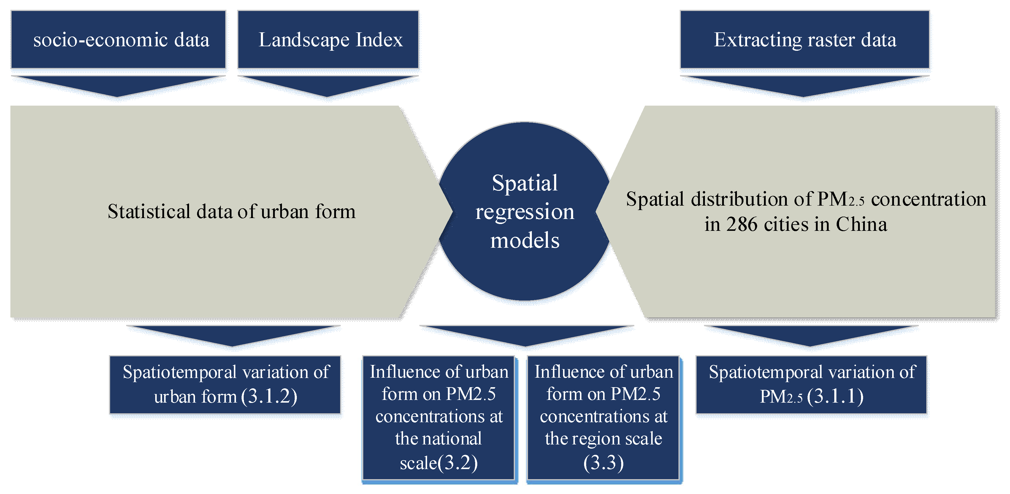
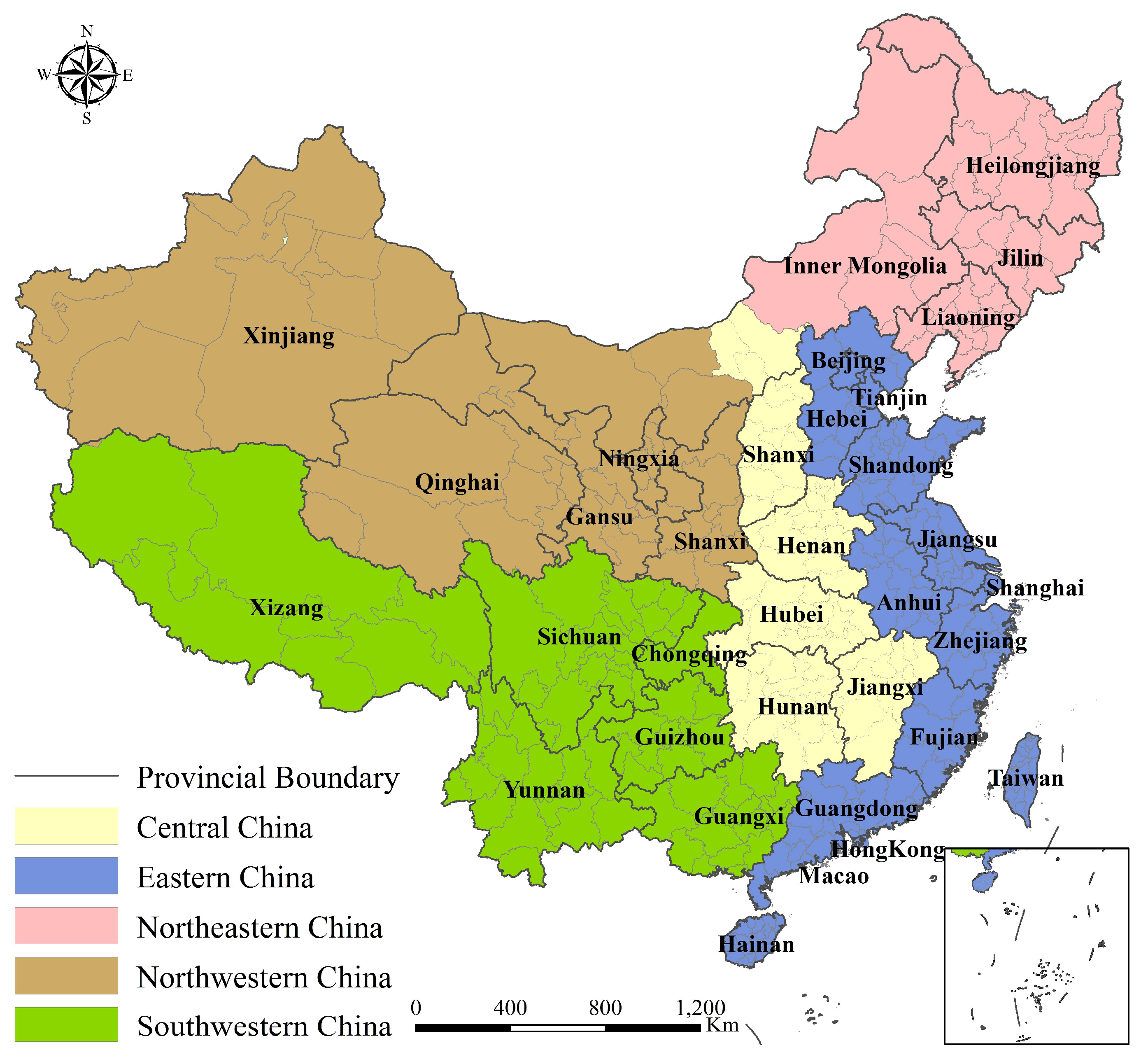
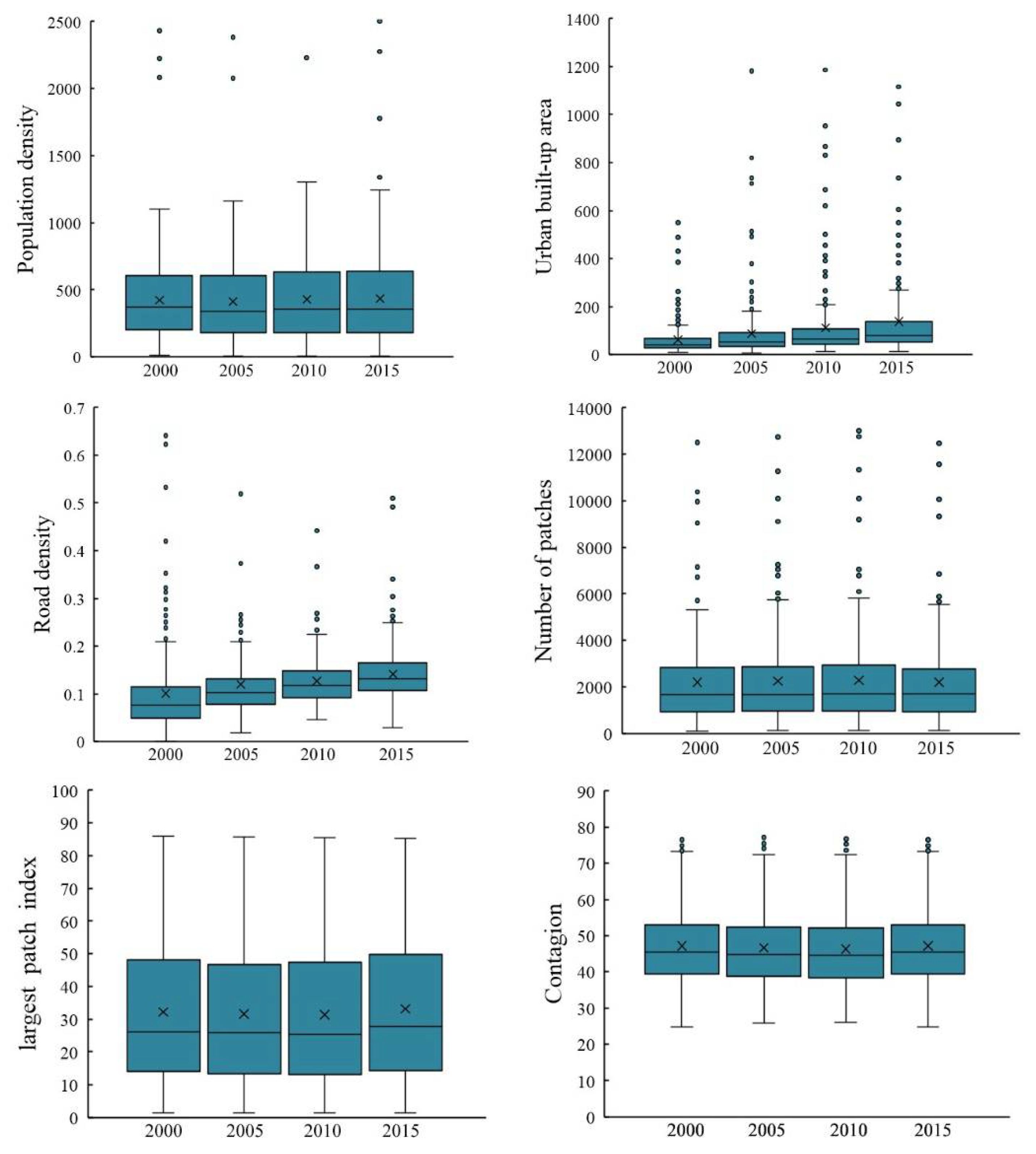
To correct the deviation in space, a spatial econometric model was used to analyze the impact of urban form on air quality in 286 cities in China. Moreover, spatial autocorrelation and spatial regression were conducted to distinguish the correlations between urban form and air quality in different regions of China. The index of urban form can be divided into two categories: a socioeconomic index and an urban landscape index. The urban landscape index was based on land-use data derived from satellites and calculated by FRAGSTATS software. According to their economic situations, the 286 prefecture level cities are divided into five regions, namely the eastern region, the central region, the northeastern region, the northwestern region, and the southwestern region. Then, the cities are divided into large cities, medium-sized cities, and small cities according to their populations. Considering China’s national conditions and the distribution of data samples, cities with a population of 3 million or below are defined as small cities. Cities with a population of 3 million to 5 million are defined as medium-sized cities. Cities with a population of more than 5 million are defined as large cities.

This study differs from existing studies in the following aspects: (1) it conducted long-term spatiotemporal analyses of PM_2.5 concentrations annually in 286 prefecture-level cities in China. (2) The urban landscape index and urban socioeconomic index were used to characterize urban form. (3) On the one hand, when the road density low, the development of road traffic is conducive to reducing PM_2.5 concentration. On the other hand, when road traffic develops to a very high level, increasingly crowded roads will increase PM_2.5 concentration. (4) Excluding the effects of meteorological and geographic conditions, most of the more-developed cities or areas, which have a higher degree of urban development (except for fragmentation, other urban-form indicators have less of an impact on PM_2.5), should exhibit moderately decentralized and polycentric urban development. (5) For less-developed cities and shrinking cities, the single-center development model can better mitigate PM_2.5 pollution than the multicenter development model. The above points define the specificity of this study. The research results will further analyze the relationship between urban morphology and PM_2.5 concentration in combination with existing relevant research so as to provide a reliable reference for urban planning and urban air quality improvement. This paper is separated into five parts: the first part contains the introduction and research objectives; the second part contains the research methods and data sources; the third part contains the data sources and variable calculations; the fourth part contains the analysis and discussion; and the fifth part contains the conclusions and research prospects with a detailed discussion of the study’s limitations. The flow chart of the article is shown in Figure 1.

2. Materials and Methods

2.1. Data Source and Variable Calculations

2.1.1. Study Area

Prefecture-level cities, with large urban area and population scale, have advantages in terms of their economic structure and geographical location. They are not only present in all parts of China but reflect the development trend of urbanization and regional economic characteristics [24]. In this study, 286 prefecture-level cities were selected as our sample. According to the degree of urban development in different regions and the different climatic and geographical conditions, Chinese cities are divided into the eastern region, central region, northeastern region, northwestern region, and southwestern region. Development of the above areas was uneven. The eastern regions have large cities, strong economic strength, and high population density [26]. Being the most developed area of China, the eastern region consumes large amounts of natural resources to maintain urban development and socioeconomic growth. The situation is similar in the eastern and central regions. Relative to the eastern and central regions, on the one hand development of the northeastern and northwestern regions is unbalanced, on the other hand problem of population loss is serious in those area. Most cities in northeastern China are resource-based or resource-exhausted. Urban development has stagnated, and cities have contracted. The degree of urban development in northwestern China is low; most cities are in a stage of rapid or embryonic development, and the urban compactness and the stability of their spatial structure are low. It is worth thinking about how the PM_2.5 concentration increased between 2000 and 2015 in two regions. To cut down PM_2.5 concentration, it is essential to determine the relationship between urban form and PM_2.5 concentration in five different regions. Furthermore, through the comparison between countries and regions, we can better understand the impact of different urban forms on PM_2.5 concentration and provide better suggestions for decision makers to reduce PM_2.5 concentration. The classification of the study area is shown in Figure 2.

2.1.2. PM_2.5 Concentration Data

The PM_2.5 concentrations in prefecture-level cities between 2000 and 2015 were taken from the dataset provided by Donkelaar’s team [27]. This dataset combines the AOD inversion results from multiple satellite instruments. The geochemical transport model was used to correlate the total column measurements of aerosols with the near-surface PM_2.5 concentration. The geographically weighted regression model (GWR) was combined with the global ground survey to adjust the residual PM_2.5 bias [27]. The gridded data was set at 0.01 degrees. Compared with 210 ground-monitoring data from North America and Europe, this dataset showed a high degree of consistency (R2 = 0.81) [28]. The detection of PM_2.5 concentration by the China Environmental Monitoring Station depends on the ground detection of air monitoring stations in each city. There are three methods for measuring PM_2.5 concentration in China’s air monitoring stations. The methods include the β Ray plus dynamic heating system method, the β Ray plus dynamic heating system combined with light scattering method, and the micro oscillating balance plus film dynamic measurement system method [29]. Compared with ground monitoring data (data from air monitoring stations in different cities), satellite measurement has both advantages and disadvantages. Since some of China’s cities lacked air monitoring stations between 2000 and 2015, one of the advantages of this method is that it can measure PM_2.5 concentrations in more cities. Its disadvantage is that it has low accuracy in areas with high reflectivity, such as snow-covered areas and is prone to extreme values. This will cause the PM_2.5 concentrations in snow-covered areas (e.g., some cities in northern China, particularly in Xinjiang and Heilongjiang Provinces) to be lower than they should be.

2.1.3. Urban Form Metrics

The urban form indicators were divided into two categories: urban index and landscape metric. The urban index is composed of urban built-up area (UA), population density (PD), and road density (RD). Urban built-up area (UA) reflects the degree of urban development. Population density (PD) represents the intensity of human social activities in a city. Road density (RD) reflects the development of a city’s transportation infrastructure and can also represent the horizontal development of a city. The above three factors were obtained from the Chinese City Statistical Yearbook from 2000 to 2015 [30]. Landscape metric is extremely useful for describing urban forms. It has several advantages for characterizing the heterogeneity of urban landscapes and the gap between urban land use patterns and governance processes, as well as analyzing urban development [31,32,33,34]. Three landscape metrics were ultimately selected to indicate urban forms in this study. These metrics were number of patches (NP), largest patch index (LPI), and contagion index (CONTAG). NP describes the heterogeneity of the whole urban landscape and represents the degree of fragmentation of urban patches. LPI represents the proportion of the largest urban patch to the whole urban landscape area. It reflects the direction and strength of human activities. CONTAG describes the agglomeration degree or extension trend of different urban patches in the landscape. The high value of CONTAG indicates that some urban patches in the landscape show good connectivity; otherwise, it indicates that the city has a dense pattern. Urban landscape data were derived from land-use datasets (30 m × 30 m) for China from 1998 to 2015 that were produced by the Institute of Remote Sensing and Digital Earth at the Chinese Academy of Sciences through the interpretation of Landsat TM or ETM images. The overall accuracy of classification for these datasets is more than 85% [35]. We used Fragstats 4.2 to calculate three urban landscape indicators for each city.

2.2. Methods

2.2.1. Spatial Autocorrelation Test

Moran’s I statistic is one of the most commonly adopted measures for spatial autocorrelation. It has been used to test spatiotemporal characteristics by identifying spatial correlations and spatial heterogeneity [36]. When researching spatial correlations and spatial distribution patterns, respectively, we usually divide Moran’s I into global Moran’s I and local Moran’s I [37]. The global Moran index describes the average correlation degree of all spatial units with the entire surrounding region, allowing us to explore whether there is spatial correlation at the regional level. The equation for calculating global Moran’s I is as follows:

$$I_G=\frac{n}{{\sum }_{i=1}^n{\sum }_{J=1}^n{W}_{ij}}\times \frac{{\sum }_{i=1}^n{\sum }_{j=1}^n{W}_{ij}\left(y_i-\overline{y}\right)\left(y_j-\overline{y}\right)}{{\sum }_{i=1}^n{\left(y_i-\overline{y}\right)}^2}$$

(1)

where $y_i$ and $y_j$ represent the attribute values of the ith spatial element and the jth spatial element, respectively; $\overline{y}$ denotes the mean value of $y$; $n$ is the total number of spatial elements; and $W_{ij}$ is the spatial weight value.

The local Moran index can be used to observe the spatial aggregation in the local areas. The equation for calculating local Moran’s I is as follows:

$$I_L=\left(y_i-\overline{y}\right){\displaystyle \sum }_{i\ne j}^n{W}_{ij}\left(y_j-\overline{y}\right)$$

(2)

The values of global Moran index and local Moran index both range from −1 to 1. For the global Moran index, when $I_G>0$, it means that the attribute values of all regions are positively correlated; otherwise, the attribute values of all regions are negatively correlated. For the local Moran index, an $I_L$ value above zero means that the indicators of a city are similar to those of surrounding cities. An $I_L$ value below zero means that a city is surrounded by cities with different indicators. To clarify the spatial aggregation of each urban form index, we generated a LISA cluster map in GeoDa on the basis of the Moran scatter diagram and the Moran index.

2.2.2. Spatial Regression Models

Regression analysis has been used in most studies to explore the relationship between urban form and PM_2.5 concentration [27,35,38,39]. Some regression analyses ignore the influence of spatial heterogeneity, such as least-squares regression analysis and ridge regression analysis [24]. A multitude of studies has proven that the spatial regression model can effectively solve the spatial dependence issue [40]. There are two commonly used spatial regression models: the spatial lag model (SLM) and the spatial error model (SEM). The calculation formula is as follows:

$$y=\mathsf{\rho }\mathrm{Wy}+\mathrm{X}\mathsf{\beta }+\mathsf{\epsilon }\left(\mathrm{SLM}\right)$$

(3)

$$y=\mathsf{\gamma }\mathrm{W}\mathsf{\epsilon }+\mathrm{X}\mathsf{\beta }+\mathsf{\delta }\left(\mathrm{SEM}\right)$$

(4)

where $y$ represents the PM_2.5 concentration of each prefecture-level city; $\mathsf{\rho }$ is the spatial lag coefficient of urban forms; $W$ represents the spatial weight; $X$ represents the urban form index; $\mathsf{\beta }$ represents the regression coefficient vector; $\epsilon$ denotes the random error vector; $\gamma$ is the residual correlation parameter, and $\delta$ represents a vector of the error terms. To determine which model to use, mainly relied on the Lagrange multiplier (LM) test and the robust LM test.

3. Results

3.1. Spatiotemporal Characteristics Analysis

3.1.1. Spatiotemporal Variation of PM_2.5

As shown in Figure 3, the average annual concentration of PM_2.5 surged from 32.34 μg/m³ in 2000 to 47.33 μg/m³ in 2015; a growth rate of 46.7%. The mean value as a whole showed a trend of first increasing and then decreasing, and the median also showed the same trend. The median values for 2000, 2005, 2010, and 2015 were 29.85 μg/m³, 47.3 μg/m³, 47.1 μg/m³, and 45.4 μg/m³, respectively. It is worth noting that the mean is always greater than the median. This indicates that there are some cities with more serious PM_2.5 pollution, making the mean value larger. In addition, PM_2.5 concentrations increased sharply in 2000–2005. The annual growth rate of the average concentration of PM_2.5 was more than three times that of the entire 15 years. The change in PM_2.5 concentration standard-reaching rate between cities also illustrates this point. In China’s ambient air quality standards, the concentration limit of fine particulate matter (PM_2.5) is divided into level I and level II, of which the level I standard is 15 μg/m³. This standard applies to areas such as nature reserves. The secondary standard is 35 μg/m³. This standard applies to residential areas, commercial areas, and other areas. In 2000, only 97 of 286 prefecture-level cities had PM_2.5 concentrations exceeding 35 μg/m³, with a standard-reaching rate of 66%. However, 225 cities had PM_2.5 concentrations above 35 μg/m³ in 2005, and the standard-reaching rate was only 21.1%. Among the 286 prefecture-level cities, the number of cities that met the Grade II Standards was 189, 61, 69, and 78 in 2000, 2005, 2010, and 2015, respectively. For detailed data on PM2.5 concentration, see Table S1 in the Supplementary Materials.

As shown in Figure 4, the distribution of PM_2.5 gradually concentrated in some areas (the northeastern region, the central region, and the eastern region). The northeastern region exhibited a high concentration of PM_2.5 in 2015. This scenario could be attributed to the coal consumption and winter heating in that region. A similar problem is also present in developed European countries. In Poland, for example, solid fuel heating in Krakow causes air pollution in surrounding cities [41]. PM_2.5 levels were also extraordinarily high in some cities in Central China, especially in the BTH region. This may be due to most cities in the central region being dependent upon secondary industries for their economic activities [42]. Additionally, heavy vehicle emissions also lead to an increase in PM_2.5 concentrations [43]. Apart from the above factors, the PM_2.5 pollution level in cities can be significantly affected by the pollution levels of their neighboring areas, especially in cities with high concentrations [44,45].

The spatial autocorrelation was weaker in 2000 (Moran’s I = 0.734) than in 2005 (Moran’s I = 0.777), 2010 (Moran’s I = 0.78), and 2015 (Moran’s I = 0.779). The trend of the change in spatial autocorrelation was the same as that of PM_2.5 concentration. As shown in

Table 1. Results of the spatial autocorrelation analysis.

Years	PM2.5
	Moran’s I	Z-score
2000	0.734	17.8813
2005	0.777	18.9055
2010	0.78	19.0748
2015	0.779	19.039

.

3.1.2. Spatiotemporal Variation of Urban Form

As is shown in Figure 5, the population density of all cities increased slightly from 423.4 in 2000 to 433.9 in 2015, indicating that the urban population has become more concentrated over the past two decades. Urban built-up areas also became larger during this period, as is indicated by the urban area index, which increased from 61.69 in 2000 to 137.21 in 2015. Road density increased from 0.1 in 2000 to 0.14 in 2015, reflecting the concentration of traffic and the degree of urban development. The number of patches showed a trend of increasing first and then decreasing, from 2206.1 in 2000 to 2278.7 in 2010 to 2209.3 in 2015, indicating that the urban form experienced dispersion and aggregation as cities developed. The trend of the largest patch index and contagion also reflects this situation. The largest patch index initially decreased from 32.17 in 2000 to 31.37 in 2010, followed by an increase to 33.14 in 2015. Contagion decreased initially from 47.1 in 2000 to 46.4 in 2010 but then increased to 47.2 in 2015. The trends of these three types of indicators indicate that the development of prefecture-level cities changed from decentralization to centralization. The contiguity and compactness of urban areas as a whole have increased.

The LISA cluster map of urban form in Chinese cities from 2000 to 2015 is shown in Figure 6. As can be seen, the spatial distribution of population density had hardly changed. From the graph, high–high clusters of population density mainly exist in the eastern region, while low–low clusters of population density exist in the northeast, the northwest, and Guangxi. The main changes were concentrated in Shaanxi Province and Henan Province. From 2000 to 2015, the spatial aggregation of population density in Shaanxi Province became stronger, while that of Henan province became weaker. On the whole, urban built-up areas can be divided into four categories of spatial pattern.

High–high clusters of urban built-up areas exist in the BTH (Beijing, Tianjin, and Hebei) region and Yangtze River Delta region (Shanghai, Zhejiang, and Jiangsu); low–low clusters of urban built-up areas exist in Shanxi, Ningxia, and central Gansu; high–low clusters of urban built-up area exist in the southeast coastal regions, including Guangxi and Guangdong; and low–high clusters of urban built-up area exist in central Liaoning and Jilin and some areas of Sichuan, Guizhou, and Hebei. The spatial aggregation changes of urban construction land are mainly concentrated in Hebei, Guangxi, and Chongqing. From the figure, we can see that the spatial distribution of traffic density in Shandong, Zhejiang, and Jiangsu is relatively concentrated. The spatial distribution of road density varies greatly from 2000 to 2015. The spatial aggregation of traffic density in Heilongjiang Province and Jilin province changed from insignificant to low–low clusters between 2000 and 2005. Shaanxi Province exhibited a high concentration in 2015. As time has gone on, the low–low clusters in Sichuan, Shanxi, Hunan, and Hubei have disappeared and some new clusters and outliers have emerged.

3.2. Influence of Urban Form on PM_2.5 Concentrations at the National Scale

It can be seen from

Table 2. The results for cities grouped by urban size (nation-wide).

Variables	LnPM2.5
	All Cities				Large				Medium				Small
	2000	2005	2010	2015	2000	2005	2010	2015	2000	2005	2010	2015	2000	2005	2010	2015
UA	0.015 **	0.01 **	0.008 **	0.009 ***	−0.007	−0.001	−0.003	0.002	−0.011	0.044 **	0.033 **	0.011	−0.003	−0.017	−0.018	−0.002
PD	0.002	0.006 **	0.003	0.006 ***	0.002	0.003	0.002	0.004	0.001	−0.004	0.014 **	0.001	0.006 **	0.023 ***	0.02 ***	0.022 ***
RD	−7.516 *	−2.018	14.886 **	22.432 ***	−4.982	−8.602	6.667	39.71 **	−5.628	1.614	7.743	−1.257	1.53	75.114 ***	33.068	29.285 **
NP	−0.001	−0.001	−0.001	−0.001	0.001	−0.001	0.001	0.001	−0.001 *	−0.002 ***	−0.001	−0.002 ***	−0.001 *	−0.001 **	−0.001 **	−0.001 *
LPI	0.056	0.085 *	0.101 **	0.191 **	0.145 *	0.349 ***	0.202 **	0.063	0.069	0.012	0.038	−0.033	0.094	0.074	0.179 *	0.098
CONTAG	−0.049	−0.119	−0.186 *	0.067	−0.215	−0.642 ***	−0.431 **	−0.082	0.094	0.18	0.302	0.498 **	0.175	0.09	−0.093	0.175
R2	0.739	0.787	0.804	0.797	0.767	0.673	0.752	0.772	0.519	0.546	0.612	0.602	0.63	0.603	0.595	0.58
S	6.566	7.554	7.648	8.4302	6.854	8.348	7.789	8.263	8.015	8.09	8.337	9.935	8.104	9.7	11.29	11.486
LogL	−972.14	−1018.141	−1027.645	−1049.404	−286.54	−316.188	−356.822	−382.965	−276.332	−303.457	−286.601	−289.524	−448.026	−423.148	−414.448	−408.91
AIC	1958.39	2050.28	2069.29	2112.81	587.095	646.378	727.644	779.93	566.665	620.915	587.202	593.048	894.053	860.296	842.897	831.833
SC	1983.91	2075.83	2094.86	2138.35	603.857	663.558	745.739	798.441	583.162	638.013	603.877	609.363	913.794	879.388	861.607	850.344
Lag coeff	0.883	0.9	0.915	0.901	0.806	0.696	0.779	0.776	0.423	0.509	0.408	0.596	0.638	0.59	0.5	0.578

Notes: *** represents a significance level of 1%, ** represents a significance level of 5%, and * represents a significance level of 10%. The urban population of large cities is more than 5 million, the urban population of medium cities is more than 3 million and less than 5 million, and the urban population of small cities is less than 3 million.

that the test results of the correlation coefficient (R2), bass information content criterion (SC), log likelihood (log likelihood), and Akaike info criterion (AIC) are significant, which proves that SEM has relatively high goodness of fit and can accurately evaluate the influence of urban form on the long-term variations in PM_2.5 concentration. From the perspective of all cities in China, not all urban form indicators are significantly correlated with PM_2.5 concentration. Specifically, UA (0.015 in 2000 and 0.009 in 2015) was significantly positively correlated with PM_2.5 concentrations. RD showed a negative correlation in 2000 (−7.516) and a significant positive correlation in 2015 (22.432) with PM_2.5 concentrations. This phenomenon shows that when the urban road density is at a low level, increasing road construction will reduce road congestion and lead to a decrease in PM_2.5 concentration, while when the urban road density is at a higher level, increasing road construction will increase the concentration of PM_2.5. In general, urban expansion and urban road network density have become the major factors impacting PM_2.5 concentrations in all cities in China.

3.3. Influence of Urban Form on PM_2.5 Concentrations at the Region Scale

The spatial regression results of five regions by city size are shown in

Table 3. The results for eastern cities grouped by urban size.

Variables	LnPM2.5
	All Cities				Large				Medium				Small
	2000	2005	2010	2015	2000	2005	2010	2015	2000	2005	2010	2015	2000	2005	2010	2015
UA	0.013	0.009	0.013 *	0.002	0.014	0.005	0.001	0.004	0.004	0.086	0.201 **	0.099 ***	0.001	−0.002	−0.102 **	−0.095 **
PD	−0.006 *	−0.004	−0.007 *	0.001	−0.009	−0.008	−0.005	0.003	−0.003	−0.021 *	−0.042 **	−0.012	−0.003	0.001	0.015 *	0.011
RD	−21.21 ***	−1.5	−2.827	21.072	−29.64 **	−4.61	−16.525	20.256	−13.07	−1.369	−74.321 *	82.627 **	20.083	143.258	273.229 ***	133.773 ***
NP	−0.001	−0.001	−0.001	0.001	−0.003 **	−0.004 ***	−0.003 **	−0.002 **	0.001 **	−0.002 **	−0.007 ***	−0.003 **	−0.001	−0.005	−0.004 ***	−0.004 **
LPI	−0.025	0.008	0.022	0.018	0.062	0.246 **	0.106	0.048	0.052	0.027	0.351	0.146	−0.05	0.081	0.264	0.524 ***
CONTAG	0.182	−0.026	−0.006	0.033	−0.021	−0.549 **	−0.227	−0.058	−0.248 **	−0.123	−0.411	−0.085	0.174	0.039	0.119	−0.733 **
R2	0.673	0.746	0.802	0.836	0.618	0.695	0.685	0.764	0.81	0.801	0.854	0.861	0.246	0.607	0.734	0.627
S	4.982	5.256	6.071	5.753	6.042	5.501	7.236	6.459	3.095	4.498	5.396	5.307	6.543	6.781	6.867	8.825
LogL	−245.994	−253.78	−262.354	−259.667	−117.522	−107.107	−119.776	−133.269	−56.653	−61.522	−49.675	−53.991	−82.527	−80.103	−78.166	−80.139
AIC	505.988	521.567	538.708	533.335	249.041	228.201	253.552	280.538	127.315	137.052	113.352	121.981	181.057	176.206	170.334	174.278
SC	522.481	538.067	555.205	549.832	244.255	238.674	264.236	292.183	134.274	144.021	118.76	127.813	190.812	185.631	178.282	181.915
Lag coeff	0.871	0.943	0.893	0.925	0.653	0.674	0.652	0.701	0.803	0.667	0.003	0.508	0.180	0.197	−0.789	0.668

Notes: *** represents a significance level of 1%, ** represents a significance level of 5%, and * represents a significance level of 10%. The urban population of large cities is more than 5 million, the urban population of medium cities is more than 3 million and less than 5 million, and the urban population of small cities is less than 3 million.

,

Table 4. The results for central cities grouped by urban size.

Variables	LnPM2.5
	All Cities				Large				Medium				Small
	2000	2005	2010	2015	2000	2005	2010	2015	2000	2005	2010	2015	2000	2005	2010	2015
UA	−0.018	0.021	0.009	0.008	−0.061	−0.032 *	−0.011	−0.005	−0.105 **	−0.038	−0.003	0.006	−0.058	−0.033	−0.012	−0.059
PD	0.012 *	0.014 **	0.014 ***	0.013 ***	0.008	0.007	0.006	0.012 ***	0.034 **	0.007	0.021	0.01	0.009	0.015 *	0.029 ***	0.027
RD	−27.656 *	18.172	16.434	40.269 **	4.139	6.533	36.294	16.302	36.126	130.853 **	158.854 *	11.315	17.782	37.505	−19.837	−2.604
NP	−0.001	−0.001	−0.001	−0.001	−0.004 ***	−0.004 ***	−0.002 **	−0.001	−0.001	−0.004 ***	−0.002	−0.006 **	−0.001	−0.004 **	0.003	0.001
LPI	0.037	0.009	0.013	−0.042	0.177	0.211 ***	−0.032	−0.037	−0.167	0.359 **	0.518	−0.008	−0.194	−0.229	−0.226	−0.284
CONTAG	−0.012	−0.065	−0.015	0.071	−0.699 **	−0.687 ***	−0.188	−0.03	0.226	−0.487	−0.665	0.203	0.654	0.488 *	0.548 *	0.733
R2	0.625	0.545	0.603	0.615	0.804	0.908	0.813	0.816	0.636	0.728	0.691	0.703	0.289	0.511	0.48	0.604
S	7.516	7.259	7.329	7.339	5.706	2.92	4.655	4.599	7.191	5.915	7.395	7.347	9.728	7.119	7.023	6.827
LogL	−274.394	−267.741	−268.577	−269.07	−89.998	−75.57	−105.614	−113.3	−78.233	−75.343	−68.877	−62.164	−103.48	−91.346	−81.016	−76.902
AIC	562.788	551.481	553.154	554.139	193.998	165.141	225.229	242.601	170.468	164.687	151.755	138.329	222.962	198.693	176.032	169.805
SC	579.285	570.335	572.007	572.993	203.069	174.467	235.913	255.488	178.416	172.636	158.726	144.562	233.62	209.06	184.279	178.889
Lag coeff	0.742	0.501	0.507	0.54	0.785	0.839	0.784	0.754	0.193	−0.534	−0.332	−0.459	0.11	0.095	0.285	0.162

Notes: *** represents a significance level of 1%, ** represents a significance level of 5%, and * represents a significance level of 10%. The urban population of large cities is more than 5 million, the urban population of medium cities is more than 3 million and less than 5 million, and the urban population of small cities is less than 3 million.

,

Table 5. The results for northeastern cities grouped by urban size.

Variables	LnPM2.5
	All Cities				Large				Medium				Small
	2000	2005	2010	2015	2000	2005	2010	2015	2000	2005	2010	2015	2000	2005	2010	2015
UA	−0.008	−0.004	−0.003	−0.013	0.067 *	0.074 ***	0.091 ***	0.012	0.137 ***	0.042	0.021	0.046	0.019	0.018	0.021	0.002
PD	0.022 **	0.036 **	0.039 ***	0.065 **	−0.031 *	−0.021	−0.003	−0.092 ***	−0.004	0.037*	0.040 ***	0.061 *	0.032 ***	0.065 ***	0.079 ***	0.084 ***
RD	−5.019	−47.899	7.051	−3.039	93.732	111.675	39.886 **	622.913	510.859 ***	−61.046	−61.169	−82.537 *	20.319	−10.087	20.509	114.183 **
NP	−0.001	−0.001	−0.001 *	−0.001	−0.006 ***	−0.011 ***	−0.008 ***	−0.027 ***	−0.001 **	−0.002 ***	−0.002 **	−0.002* *	0.001 **	0.001 **	0.001 ***	0.002 ***
LPI	0.109 *	0.098	0.012	−0.078	−0.877 **	−1.713 **	−1.451**	−4.233 **	0.015	−0.096	−0.169	−0.723 **	0.246 ***	0.361 ***	0.391 **	0.436 **
CONTAG	−0.292 *	−0.307	−0.249	0.007	0.593 **	2.065 **	1.979 ***	4.994 ***	−0.463	−0.102	0.153	3.161 ***	−0.654 ***	−0.944 ***	−1.188 **	−1.242 ***
R2	0.529	0.633	0.688	0.586	0.844	0.881	0.904	0.897	0.872	0.489	0.616	0.942	0.656	0.705	0.715	0.686
S	3.929	5.572	6.035	10.989	2.248	3.296	2.963	5.575	2.354	5.566	5.209	3.461	3.184	4.861	5.927	7.534
LogL	−105.224	−118.119	−121.041	−142.757	−14.772	−17.063	−15.493	−20.756	−18.887	−28.266	−28.548	−26.299	−58.782	−66.497	−71.079	−76.559
AIC	224.449	250.238	256.082	299.515	37.543	42.127	38.987	49.512	45.774	66.538	65.096	60.598	125.564	140.996	150.159	161.119
SC	235.726	261.514	267.358	310.791	36.711	41.294	38.154	48.679	46.092	67.518	65.885	61.387	129.928	145.36	154.523	165.483
Lag coeff	0.626	0.623	0.618	0.555	0.836	0.836	−0.562	0.904	0.583	0.333	−0.678	−0.984	0.572	0.303	0.358	0.401

Notes: *** represents a significance level of 1%, ** represents a significance level of 5%, and * represents a significance level of 10%. The urban population of large cities is more than 5 million, the urban population of medium cities is more than 3 million and less than 5 million, and the urban population of small cities is less than 3 million.

,

Table 6. The results for northwestern cities grouped by urban size.

Variables	LnPM2.5
	All Cities				Large				Medium				Small
	2000	2005	2010	2015	2000	2005	2010	2015	2000	2005	2010	2015	2000	2005	2010	2015
UA	0.014	0.024	0.016	0.025 *	−0.001	−0.012 ***	−0.004 ***	−0.005 ***	−0.081 ***	0.009	0.017 **	0.02 ***	0.042	0.109 ***	0.057 ***	0.064 ***
PD	0.036 ***	0.047 ***	0.041 ***	0.034 ***	−0.001	−0.008	−0.003 ***	−0.005 ***	0.063 ***	0.081	0.01	0.001	0.001	0.056 **	0.046 ***	0.03*
RD	−23.437 ***	−29.944	1.601	15.619	2.042	−10.758	−2.625	2.827	−130.714 ***	−5.359	4.309	45.063 ***	3.974	−24.226	17.923	0.546
NP	0.001 **	0.001	0.001	0.001	−0.001 ***	0.004	−0.003 **	−0.003	0.001 *	−0.005 *	0.001	−0.002	−0.001	0.001	0.001	0.001
LPI	0.023	0.166	0.222	0.146 *	−0.003	0.102 ***	0.025	0.048 ***	0.199 **	0.262	0.185	0.049	−0.108	0.145	0.067	0.112 *
CONTAG	0.484 *	0.543 *	0.235	0.536 ***	−0.001	0.204 **	0.06 *	0.142 **	1.011 **	−0.227	−2.498 ***	−0.315	0.079	0.044	−0.06	0.002
R2	0.783	0.818	0.799	0.767	0.767	0.854	0.895	0.851	0.944	0.847	0.924	0.971	0.582	0.639	0.683	0.745
S	5.164	6.43	5.611	6.19	0.604	0.701	0.675	0.572	1.168	4.482	1.09	0.848	4.176	6.11	4.368	4.206
LogL	−99.016	−108.175	−102.893	−105.546	1.832	−3.885	−2.952	−1.98	−12.1	−21.478	−14.001	−12.889	−63.912	−76.4	−65.835	−63.878
AIC	214.033	230.349	219.786	225.093	0.334	11.77	3.46	7.978	34.2	50.957	36.003	33.779	141.824	166.801	145.672	141.757
SC	225.759	240.609	230.046	235.354	−1.467	9.967	1.657	6.175	33.93	50.741	35.787	33.562	149.461	174.749	153.309	149.394
Lag coeff	0.483	0.752	0.664	0.603	−0.33	−0.33	−0.33	−0.33	0.693	0.752	0.956	0.975	0.571	0.669	0.713	0.533

Notes: *** represents a significance level of 1%, ** represents a significance level of 5%, and * represents a significance level of 10%. The urban population of large cities is more than 5 million, the urban population of medium cities is more than 3 million and less than 5 million, and the urban population of small cities is less than 3 million.

and

Table 7. The results for southwestern cities grouped by urban size.

Variables	LnPM2.5
	All Cities				Large				Medium				Small
	2000	2005	2010	2015	2000	2005	2010	2015	2000	2005	2010	2015	2000	2005	2010	2015
UA	0.032	0.008	0.013	−0.005	0.048 ***	0.007	0.023	0.01	−0.016	−0.073*	0.113 **	0.023	0.054	−0.309 **	−0.686 ***	0.038
PD	0.006	0.013	0.016 **	0.013 *	0.01 *	0.008	0.009	0.011	−0.007	−0.017 *	−0.035	−0.009	−0.005	−0.024	0.008	−0.031 ***
RD	−2.569	−0.514	−11.826	21.076	17.775 **	−92.773 **	−36.323	68.443 *	−41.895 ***	50.484 *	−118.929	−14.477	−6.993	45.942	115.688 *	34.418 ***
NP	0.001	0.001	0.001	0.002 **	0.002 **	0.001	0.007	0.002 *	−0.003	0.001	−0.006*	−0.003	−0.001	−0.002	−0.001	−0.001
LPI	−0.002	0.121	0.14	0.153	0.411	1.115 ***	0.48	0.723 ***	−0.199	0.063	−0.103	−0.06	−0.071	−0.078	0.336*	0.269 ***
CONTAG	0.069	−0.273	−0.116	−0.3	−0.387	−1.335 **	−0.354	−1.163 ***	0.308	−0.533 *	1.096 *	0.339	0.248	0.325	−0.651	−0.52 ***
R2	0.523	0.709	0.78	0.664	0.809	0.734	0.525	0.664	0.653	0.797	0.717	0.301	0.159	0.817	0.699	0.952
S	5.009	7.26	6.242	5.113	2.462	6.108	7.911	4.173	2.133	3.752	5.823	5.655	6.436	4.719	5.567	1.878
LogL	−138.356	−157.129	−149.6	−141.425	−20.904	−39.531	−55.821	−46.427	−36.308	−57.09	−55.285	−50.523	−66.051	−46.312	−41.318	−32.658
AIC	292.713	330.257	315.2	296.851	51.808	93.062	127.643	106.854	86.617	128.18	124.571	117.048	146.103	106.624	98.637	79.316
SC	307.166	344.711	329.654	309.497	52.794	96.457	134.791	112.262	92.025	134.791	129.979	123.228	153.073	111.097	103.157	83.271
Lag coeff	0.492	0.663	0.613	0.669	0.125	0.503	0.82	0.449	−0.608	0.82	0.82	0.161	0.29	0.823	−0.396	0.924

Notes: *** represents a significance level of 1%, ** represents a significance level of 5%, and * represents a significance level of 10%. The urban population of large cities is more than 5 million, the urban population of medium cities is more than 3 million and less than 5 million, and the urban population of small cities is less than 3 million.

. Some coefficients of the influence of urban form on PM_2.5 concentration in eastern and central China are basically consistent with the national results. For instance, the increase in urban built-up area promoted the increase in PM_2.5 concentrations in the eastern cities, especially in 2000. In addition, for the eastern cities, road density showed a negative correlation with PM_2.5 concentration in 2000, but the results were reversed in 2015; there was a positive correlation (Table 3). The reasons for this are manifold. On the one hand, the increase in road density is closely related to economic development. On the other hand, as roads become more developed, the compactness of cities will also increase correspondingly, further affecting PM_2.5 concentration.

In the northeastern region, only PD had a significant correlation with PM_2.5 concentration between 2000 and 2015 (0.022 in 2000 and 0.065 in 2015). However, when the analysis was refined according to the size of the cities, the results were different. For large and small cities in northeastern China, in addition to PD, the impact of NP, LPI, and CONTAG on PM_2.5 was also significant. It is worth noting that NP and LPI were negatively correlated with PM_2.5 concentration in large cities, while CONTAG was positively correlated with PM_2.5. The opposite was true of small cities (Table 5). Cities in the northwest faced the same situation as those in the northeast. PD was still the most important factor affecting PM_2.5 concentration in northwestern China. For small- and medium-sized cities in northwestern China, UA also played a positive role in PM_2.5 concentration, especially in 2015 (medium 0.02 and small 0.064). UA was negatively correlated with PM_2.5 concentration in large cities. Otherwise, LPI (0.048) had the greatest positive impact on PM_2.5 in 2015. This state of affairs also confirms that large cities, which have become diverse, continuous, and uncompact, have been able to reduce PM_2.5 pollution.

4. Discussion

4.1. The Relationship between PM_2.5 and Urban Areafrom a National Perspective

According to the estimated results in Table 2, several important conclusions can be drawn at the national scale. First, the correlation coefficients of urban areas (built-up areas) were significantly positive in 286 prefecture-level cities, implying that the expansion of urban areas aggravates the pollution of PM_2.5 at the national scale and especially in large cities. Liu [46] and She [21] also found a positive relationship between the urban area and urban air pollution. The emergence of this situation may be due to the expansion of the urban area, which leads to population growth and increased road traffic. These factors aggravate energy consumption and increase PM_2.5 pollution.

Second, the correlation coefficients of population density were significantly positive in 2000, 2005, and 2010 but not significant in 2015, implying that increased population density leads to more PM_2.5 pollution. An increase in population density not only increases the demand for consumption and work resources but also aggravates housing congestion and traffic jams [15].

Third, the correlation coefficients of road density were significantly negative in 2000 but positive in 2015. It is possible that the road density has a positive correlation with PM_2.5 when the road density reaches a certain limit, and the correlation increases gradually. It was found that some emerging cities that are developing show opposite results in terms of road density compared to some other large cities. For example, in Yangquan, a city located in the northwestern region of China, the road density increased from 0.095 to 0.1429 between 2005 and 2015, but the annual average concentration of PM_2.5 decreased from 63.6 μg/m³ to 57.2 μg/m³. However, further research is needed by the authors to ascertain exactly what this limit is and whether it is more relevant to industrial development or to urban planning.

Fourth, the correlation coefficient of NP in small- and medium-sized cities is significantly and negative, but not for large cities. This shows that the impact of urban fragmentation on PM_2.5 concentration is only reflected in cities on a general scale. The correlation coefficients of the large patches index were significant and positive in 2005 and 2010. This indicates that small, dispersed, and polycentric cities exhibited less PM_2.5 pollution than compact and larger cities. A similar finding was observed by Wu et al. [32] and She et al. [21], who both concluded that a more uniform distribution of urban patches might be better for mitigating particulate matter in large urban agglomerations (for example, the YRD region). The more complex the urban form is, the greater the average distance between urban patches and the smaller the concentration of PM_2.5. This shows that the multicenter urban form can improve air quality.

Lastly, unlike previous studies, we found that urban compactness (CONTAG) does not promote PM_2.5 concentrations at the national scale. Urban connectivity, or connectivity between centers, had little effect on PM_2.5 concentrations. With an increase in the population and a change in policy, cities, especially larger cities, begin to change from a single center to a double- or multicenter model.

4.2. The Relationship between PM_2.5 and Urban Form from the Sub-Regional Perspective

From the overall situation of each region, the impact of the urban area on PM_2.5 concentration varies with city size. Compared with small- and medium-sized cities, the change in PM_2.5 concentration in big cities is more easily affected by the urban area. An increased urban built-up area corresponds to greater traffic demand and energy consumption, causing comparatively worse air quality [14,47]. The impact of the urban built-up area on PM_2.5 concentration in northwestern China is more significant. The reason for this situation may be that the cities in northwestern China are in the initial stage of development, and the rapid increase in the urban area makes PM_2.5 pollution more serious.

Additionally, the population density of the cities in the northeast and northwest has a great influence on the concentration of PM_2.5, but the population density in the east has little influence. This kind of regional difference may be caused by differences in the speed of land urbanization and population urbanization. On the one hand, the reason is that the population density of the cities in the northeast and northwest is smaller than that in the east; on the other hand, in recent years, some cities in northeastern China have been facing resource depletion contraction, which makes population density more sensitive to PM_2.5 concentration. The differences between northwestern China and northeastern China are as follows: first of all, most cities in northwestern China are in a period of rapid development; the built-up area is increasing and population growth is stagnant. The speed of land urbanization and population urbanization in northwestern cities was in a serious decoupling state: the urban land expansion speed was faster than that of the population expansion [48]. Secondly, the urban contraction in northeastern China is more serious than that in northwestern China, which has resulted in northeastern China becoming a single-core area, increasing the influence of population and road density on PM_2.5. Lastly, the northwestern region is at a high altitude and has more mountains than the northeastern region; the less compact urban form helps disperse pollutants over the mountainous terrain, which results in less urban air pollution [21,49].

The influence of patch number and maximum patch index on PM_2.5 concentration was significant in northeastern China. It is worth noting that the results of large cities are the opposite of those of small cities. The results of large cities are similar to those of other developed regions. When cities tend to be polycentric, PM_2.5 pollution is reduced. However, the results obtained by small cities are just the opposite. When cities develop intensively and reduce the degree of urban fragmentation, it is easier to reduce the concentration of PM_2.5. This result is not consistent with those obtained by other researchers. For instance, Namdeo et al. [50] found that a more compact urban layout helps to reduce urban traffic and improve industrial efficiency, thereby improving air quality. Lu and Liu indicated a negative correlation between compact urban form and air pollution in most cities of China. Bechle et al. [47] demonstrated that urban compactness was not a significant predictor of air pollution in 83 global cities. Fan et al. [39] found that a more compact urban form leads to less PM_2.5 pollution in China, especially in the northern region.

In southwestern China, the influence of urban form on PM_2.5 concentration was not significant. This may be caused by topography, weather, or industrial conditions. Most of the cities in southwestern China are concentrated in intermountain basins, river valleys, and alluvial fans, and the annual rainfall is substantial [26]. These conditions result in lower levels of air pollution in these places than in other places [42]. In addition, in southwestern China, the lack of coal industry was also an important reason for this result.

4.3. Limitations and Future Directions

There are three limitations to this study. The first is that the concentration of PM_2.5 is affected by many factors, and while it is certain that urban form is one of the key factors, other factors may play a more important role in influencing PM_2.5 concentration in some areas. For example, many of the southwestern cities are located in the mountainous valley zones, and their terrains are narrow. At the same time, rainfall is more concentrated in these areas. The terrain and meteorological factors are two of the main reasons for the changes in PM_2.5 concentration. Not all PM_2.5 pollution can be attributed to urban form. The second point is that the mechanism of influence of urban form on PM_2.5 concentration is not completely distinct, and it needs to be further studied in the future. The main reason for this is that the resolution of land-use data is low, and it is difficult to accurately determine the spatial distribution of roads, commercial areas, and residential areas through land-use data with a 1 km resolution. The calculation results of urban forms, such as the road density and patch number, may be biased. The last point is that based on data availability, our study focuses on the average annual variation in PM_2.5 concentration from 2000 to 2015. Future studies should analyze the relationship between urban forms, PM_2.5 concentrations, and seasonal variations on a spatiotemporal scale.

5. Conclusions

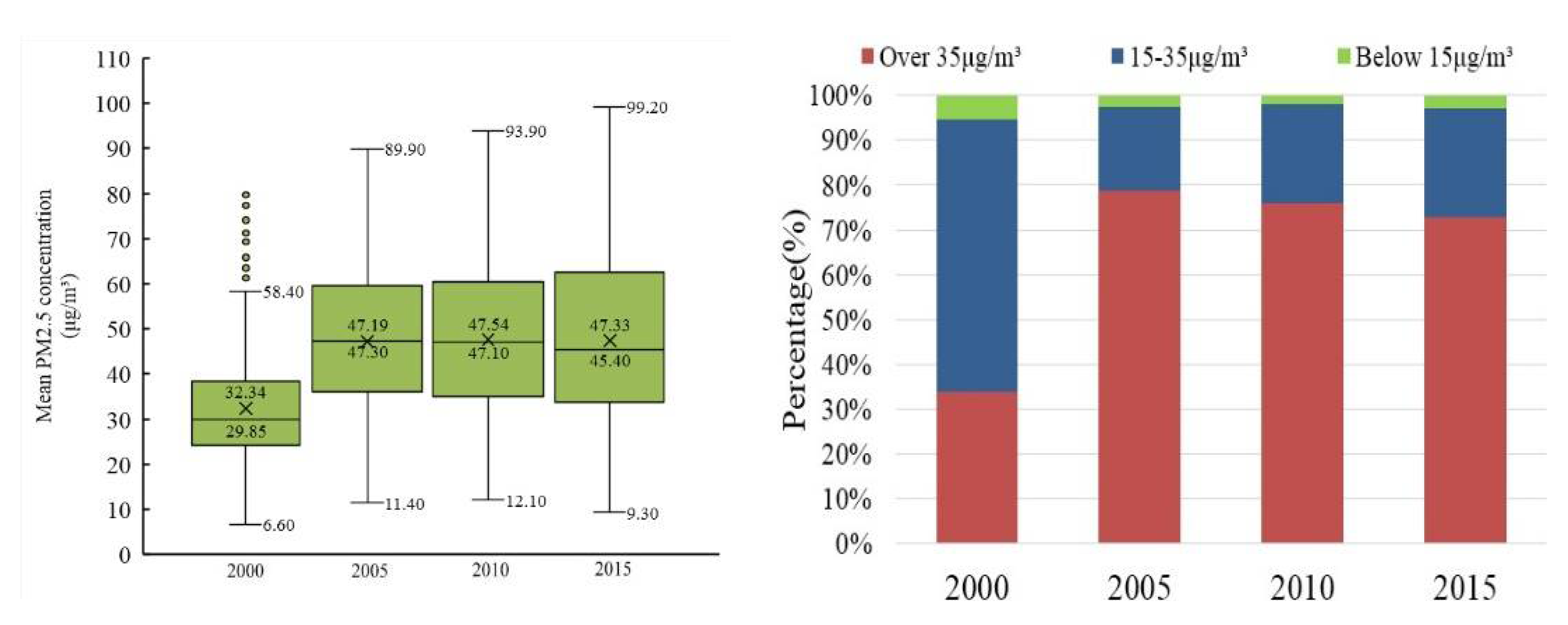
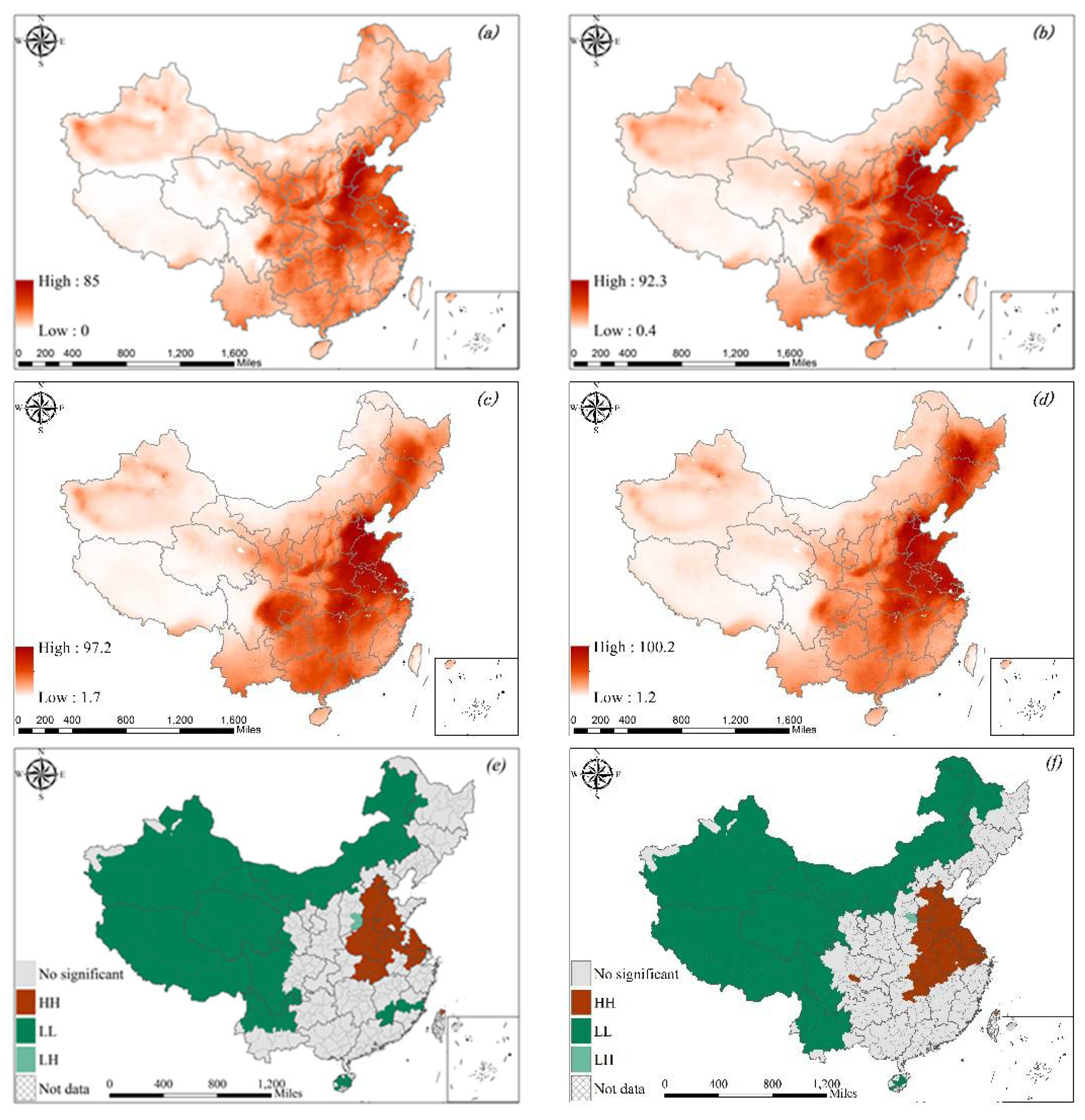
This study, using 286 prefecture-level Chinese cities as its sample data, examined the spatial patterns and temporal trends of PM_2.5 concentration from 2000 to 2015 and further explored the influence of urban form on PM_2.5 concentration. The results show that the PM_2.5 concentration significantly increased during the period from 2000 to 2005. The cities with heavy PM_2.5 pollution were mainly concentrated in the eastern and central regions of China, especially in the large cities and their surrounding areas. The cities with large changes in PM_2.5 concentration were mainly distributed in northeastern China. Specifically, many cities in the BTH and Yangtze River Delta regions, as well as central Liaoning and Shandong provinces, had more serious PM_2.5 pollution. Moreover, cities with high PM_2.5 concentrations be located close to one another, which indicates that PM_2.5 concentration is regional. From the national point of view, urban area and road density are related to higher PM_2.5 concentrations. On the other hand, there is little correlation between urban fragmentation and PM_2.5 concentration.

In the Northeast and Northwest China, the urban form and population density have more influence on PM_2.5 concentration. The reason for this is that the speed of land urbanization and population urbanization in the northeastern and northwestern regions of China was in a seriously decoupled state, and there was a serious phenomenon of urban contraction. Therefore, moderately compact and single-center urban development is conducive to the air quality of small- and medium-sized cities in northeastern and northwestern China. For the cities in the eastern and central regions, and most large-scale cities in China, it is more important to control unplanned urban and road expansion to encourage cities to develop in a decentralized and multicenter manner.

References

1. Song, C.; Wu, L.; Xie, Y.; He, J.; Chen, X.; Wang, T.; Lin, Y.; Jin, T.; Wang, A.; Liu, Y.; et al. Air pollution in China: Status and spatiotemporal variations. Environ. Pollut. 2017, 227, 334–347. [Google Scholar] [CrossRef]
2. Cohen, A.J.; Brauer, M.; Burnett, R.; Anderson, H.R.; Frostad, J.; Estep, K.; Balakrishnan, K.; Brunekreef, B.; Dandona, L.; Dandona, R.; et al. Estimates and 25-year trends of the global burden of disease attributable to ambient air pollution: An analysis of data from the global burden of diseases study 2015. Lancet 2017, 389, 1907–1918. [Google Scholar] [CrossRef] [Green Version]
3. Liu, Y.; Wu, J.; Yu, D. Characterizing spatiotemporal patterns of air pollution in China: A multiscale landscape approach. Ecol. Indic. 2017, 76, 344–356. [Google Scholar] [CrossRef] [Green Version]
4. Cheng, Z.; Jiang, J.; Fajardo, O.; Wang, S.; Hao, J. Characteristics and health impacts of particulate matter pollution in China (2001–2011). Atmos. Environ. 2013, 65, 186–194. [Google Scholar] [CrossRef]
5. Health Effects Institute. State of Global Air 2017; Special Report; Health Effects Institute: Boston, MA, USA, 2017; Available online: https://www.stateofglobalair.org/resources?resource_category=archives#block-exposedformresources-all (accessed on 16 December 2021).
6. Mansfield, T.A.; Freer-Smith, P.H. Effects of urban air pollution on plant growth. Biol. Rev. 1981, 56, 343–368. [Google Scholar] [CrossRef]
7. Lovett, G.M.; Tear, T.H.; Evers, D.C.; Findlay, S.E.G.; Cosby, B.J.; Dunscomb, J.K.; Driscoll, C.T.; Weathers, K.C. Effects of air pollution on ecosystems and biological diversity in the eastern United States. Ann. N. Y. Acad. Sci. 2009, 1162, 99–135. [Google Scholar] [CrossRef] [PubMed]
8. Smith, P.; Ashmore, M.R.; Black, H.I.J.; Burgess, P.J.; Evans, C.D.; Quine, T.A.; Thomson, A.M.; Hicks, K.; Orr, H.G. Review: The role of ecosystems and their management in regulating climate, and soil, water and air quality. J. Appl. Ecol. 2013, 50, 812–829. [Google Scholar] [CrossRef]
9. Chen, S.-M.; He, L.-Y. Welfare loss of China’s air pollution: How to make personal vehicle transportation policy. China Econ. Rev. 2014, 13, 106–118. [Google Scholar] [CrossRef]
10. Mukhopadhyay, A.; Pandit, V. Control of industrial air pollution through sustainable development. Environ. Dev. Sustain. 2014, 16, 35–48. [Google Scholar] [CrossRef]
11. Zhang, X.; Zhang, X.; Chen, X. Happiness in the air: How does a dirty sky affect mental health and subjective well-being? J. Environ. Econ. Manag. 2017, 85, 81–94. [Google Scholar] [CrossRef]
12. Du, G.; Shin, K.J.; Managi, S. Variability in impact of air pollution on subjective well-being. Atmos. Environ. 2018, 183, 175–208. [Google Scholar] [CrossRef]
13. Naboni, E.; Woźniak-Szpakiewicz, E.; Doray, C. Future cities: Design opportunities for the improvement of air quality. Czas. Tech. Archit. 2014, 111, 235–250. Available online: https://repozytorium.biblos.pk.edu.pl/resources/30538 (accessed on 16 December 2021).
14. Bereitschaft, B.; Debbage, K. Urban form, air pollution, and CO2 emissions in large U.S. metropolitan areas. Prof. Geogr. 2013, 65, 612–635. [Google Scholar] [CrossRef]
15. McCarty, J.; Kaza, N. Urban form and air quality in the United States. Landsc. Urban. Plan. 2015, 139, 168–179. [Google Scholar] [CrossRef]
16. Cárdenas Rodríguez, M.; Dupont-Courtade, L.; Oueslati, W. Air pollution and urban structure linkages: Evidence from european cities. Renew. Sustain. Energy Rev. 2016, 53, 1–9. [Google Scholar] [CrossRef]
17. Stone, B. Urban sprawl and air quality in large US cities. J. Environ. Manag. 2008, 86, 688–698. [Google Scholar] [CrossRef]
18. Clark, L.P.; Millet, D.B.; Marshall, J.D. Air quality and urban form in U.S. urban areas: Evidence from regulatory monitors. Environ. Sci. Technol. 2011, 45, 7028–7035. [Google Scholar] [CrossRef]
19. Wang, Z.; Fang, C. Spatial-temporal characteristics and determinants of PM2.5 in the Bohai Rim urban agglomeration. Chemosphere 2016, 148, 148–162. [Google Scholar] [CrossRef]
20. Li, F.; Zhou, T. Effects of urban form on air quality in China: An analysis based on the spatial autoregressive model. Cities 2019, 89, 130–140. [Google Scholar] [CrossRef]
21. She, Q.; Peng, X.; Xu, Q.; Long, L.; Wei, N.; Liu, M.; Jia, W.; Zhou, T.; Han, J.; Xiang, W. Air quality and its response to satellite-derived urban form in the Yangtze River delta, China. Ecol. Indic. 2017, 75, 297–306. [Google Scholar] [CrossRef]
22. Zhang, C.; Zhang, S. Study on urban form and air quality in metropolitan area: Identify relations and research framework. Urban Dev. Stud. 2014, 21, 47–53. [Google Scholar] [CrossRef]
23. Feng, H.; Zou, B.; Tang, Y. Scale- and region-dependence in landscape-PM2.5 correlation: Implications for urban planning. Remote Sens. 2017, 9, 918. [Google Scholar] [CrossRef] [Green Version]
24. Shi, K.; Li, Y.; Chen, Y.; Li, L.; Huang, C. How does the urban form-PM2.5 concentration relationship change seasonally in chinese cities? A comparative analysis between national and urban agglomeration scales. J. Clean. Prod. 2019, 239, 118088. [Google Scholar] [CrossRef]
25. Song, Y.; Huang, B.; He, Q.; Chen, B.; Wei, J.; Mahmood, R. Dynamic assessment of PM2.5 exposure and health risk using remote sensing and geo-spatial big data. Environ. Pollut. 2019, 253, 288–296. [Google Scholar] [CrossRef]
26. Xu, X.; Xiao, T.; Ma, S. The features analysis on divisions of season in southwest China. Plateau Mt. Meteorol. Res. 2010, 30, 35–40. [Google Scholar] [CrossRef]
27. Larkin, A.; van Donkelaar, A.; Geddes, J.A.; Martin, R.V.; Hystad, P. Relationships between changes in urban characteristics and air quality in east Asia from 2000 to 2010. Environ. Sci. Technol. 2016, 50, 9142–9149. [Google Scholar] [CrossRef] [Green Version]
28. Van Donkelaar, A.; Martin, R.V.; Brauer, M.; Boys, B.L. Use of satellite observations for long-term exposure assessment of global concentrations of fine particulate matter. Environ. Health Perspect. 2015, 123, 135–143. [Google Scholar] [CrossRef] [Green Version]
29. Ministry of Ecology and Environment the People’s Republic of China. Specifications and Test Procedures for Ambient Air Quality Continuous Automated Monitoring System for PM10 and PM2.5; Ministry of Ecology and Environment the People’s Republic of China: Beijing, China, 2013. Available online: https://www.mee.gov.cn/ywgz/fgbz/bz/bzwb/jcffbz/202201/t20220129_968586.shtml (accessed on 16 December 2021).
30. National Bureau of Statistics of China. China Statistical Yearbook; National Bureau of Statistics of China: Beijing, China. Available online: http://www.stats.gov.cn/tjsj/ndsj/ (accessed on 16 December 2021).
31. Chen, Y.; Li, X.; Zheng, Y.; Guan, Y.; Liu, X. Estimating the relationship between urban forms and energy consumption: A case study in the Pearl River delta, 2005–2008. Landsc. Urban Plan. 2011, 102, 33–42. [Google Scholar] [CrossRef]
32. Wu, J.; Xie, W.; Li, W.; Li, J. Effects of urban landscape pattern on PM2.5 pollution—A beijing case study. PLoS ONE 2015, 10, e0142449. [Google Scholar] [CrossRef] [Green Version]
33. Jaeger, J.; Nazarnia, N. Social and ecological impacts of the exponential increase of urban sprawl in Montréal. Can. Commun. Dis. Rep. 2016, 42, 207–208. [Google Scholar] [CrossRef]
34. Li, J.; Huang, X. Impact of land-cover layout on particulate matter 2.5 in urban areas of China. Int. J. Digit. Earth 2020, 13, 474–486. [Google Scholar] [CrossRef]
35. Tao, Y.; Zhang, Z.; Ou, W.; Guo, J.; Pueppke, S.G. How does urban form influence PM2.5 concentrations: Insights from 350 different-sized cities in the rapidly urbanizing Yangtze River delta region of China, 1998–2015. Cities 2020, 98, 102581. [Google Scholar] [CrossRef]
36. Dong, L.; Liang, H. Spatial analysis on China’s regional air pollutants and CO2 emissions: Emission pattern and regional disparity. Atmos. Environ. 2014, 92, 280–291. [Google Scholar] [CrossRef]
37. Zhao, L.; Sun, C.; Liu, F. Interprovincial two-stage water resource utilization efficiency under environmental constraint and spatial spillover effects in China. J. Clean. Prod. 2017, 164, 715–725. [Google Scholar] [CrossRef]
38. Lee, C. Impacts of urban form on air quality in metropolitan areas in the United States. Comput. Environ. Urban Syst. 2019, 77, 101362. [Google Scholar] [CrossRef]
39. Fan, C.; Tian, L.; Zhou, L.; Hou, D.; Song, Y.; Qiao, X.; Li, J. Examining the impacts of urban form on air pollutant emissions: Evidence from China. J. Environ. Manag. 2018, 212, 405–414. [Google Scholar] [CrossRef]
40. Fang, C.; Li, G.; Wang, S. Changing and differentiated urban landscape in China: Spatiotemporal patterns and driving forces. Environ. Sci. Technol. 2016, 50, 2217–2227. [Google Scholar] [CrossRef]
41. Danek, T.; Zaręba, M. The use of public data from low-cost sensors for the geospatial analysis of air pollution from solid fuel heating during the COVID-19 pandemic spring period in Krakow, Poland. Sensors 2021, 21, 5208. [Google Scholar] [CrossRef]
42. Zhang, Y.-L.; Cao, F. Fine particulate matter (PM2.5) in China at a city level. Sci. Rep. 2015, 5, 14884. [Google Scholar] [CrossRef] [Green Version]
43. Wang, S.; Zhou, C.; Wang, Z.; Feng, K.; Hubacek, K. The characteristics and drivers of fine particulate matter (PM2.5) distribution in China. J. Clean. Prod. 2017, 142, 1800–1809. [Google Scholar] [CrossRef]
44. Burton, R.M.; Suh, H.H.; Koutrakis, P. Spatial variation in particulate concentrations within metropolitan Philadelphia. Environ. Sci. Technol. 1996, 30, 400–407. [Google Scholar] [CrossRef]
45. Han, L.; Zhou, W.; Li, W.; Li, L. Impact of urbanization level on urban air quality: A case of fine particles (PM2.5) in Chinese cities. Environ. Pollut. 2014, 194, 163–170. [Google Scholar] [CrossRef]
46. Liu, Y.; Wu, J.; Yu, D.; Ma, Q. The relationship between urban form and air pollution depends on seasonality and city size. Environ. Sci. Pollut. Res. 2018, 25, 15554–15567. [Google Scholar] [CrossRef] [PubMed]
47. Bechle, M.J.; Millet, D.B.; Marshall, J.D. Effects of income and urban form on urban NO2: Global evidence from satellites. Environ. Sci. Technol. 2011, 45, 4914–4919. [Google Scholar] [CrossRef] [PubMed]
48. Yin, H.; Xu, T. The mismatch between population urbanization and land urbanization in China. Urban Plan. Forum 2013, 2, 10–15. [Google Scholar] [CrossRef]
49. Loo, B.P.Y.; Chow, A.S.Y. Spatial restructuring to facilitate shorter commuting: An example of the relocation of Hong Kong international airport. Urban Stud. 2011, 48, 1681–1694. [Google Scholar] [CrossRef]
50. Namdeo, A.; Goodman, P.; Mitchell, G.; Hargreaves, A.; Echenique, M. Land-use, transport and vehicle technology futures: An air pollution assessment of policy combinations for the Cambridge sub-region of the UK. Cities 2019, 89, 296–307. [Google Scholar] [CrossRef]
Figure 1. Flow chart of the article.
Sustainability 14 02187 g001
Figure 2. Study area.
Sustainability 14 02187 g002
Figure 3. Mean PM2.5 concentration and annual statistics of the proportion of days with different PM2.5 levels from 2000 to 2015.
Sustainability 14 02187 g003
Figure 4. Spatial variation of PM2.5 concentration from 2000 to 2015. (ad) show the changes of PM concentration from 2000 to 2015. (eh) show the spatial clusters of PM concentration from 2000 to 2015. Not significant indicates that the region is not significantly clustered. No data indicates that there is no data in this area.
Sustainability 14 02187 g004aSustainability 14 02187 g004b
Figure 5. Urban form metrics for 286 different-sized prefecture-level cities between 2000 and 2015.
Sustainability 14 02187 g005
Figure 6. LISA cluster map of urban index in Chinese cities from 2000 to 2015. Panels (ad) show the spatial clusters of population density between 2000 and 2015; panels (eh) show the spatial clusters of urban areas (built-up areas) from 2000 to 2015. Panels (il) show the spatial clusters of road density between 2000 and 2015. Specifically, HH indicates a city with a high population density (urban area, road density) surrounded by cities with high population density (urban area, road density); LL indicates a city with a low population density (urban area, road density) surrounded by cities with low population density (urban area, road density); HL indicates a city with a high population density (urban area, road density) surrounded by cities with low population density (urban area, road density); and LH indicates a city with a low population density (urban area, road density) surrounded by cities with high population density (urban area, road density).
Sustainability 14 02187 g006