Use of Universal Simulation Software Tools for Optimization of Signal Plans at Urban Intersections

Abstract

Intersections in cities are important transport hubs, where traffic flows from all roads meet, connect, disconnect or intersect. This research is dedicated to the creation of simulation models of intersections and is based on real observations of two crossroads in a city. The principle is based on observing traffic flows using real traffic counting at peak times. The aim is to reduce traffic congestion by adjusting signal plans on the monitored section using computer simulation and modelling in ExtendSim8 software, which is a universal tool allowing the user to simulate any system or process by creating a logical representation in an easy-to-use format. According to our preliminary literature research, the ExtendSim software has never before been used before to create an intersection simulation to optimize the signal plan. There are several specialized software products for simulating traffic and intersections, but not everyone has access to these, or else they require lengthy user training. Therefore, it is very advantageous to use a universal simulation tool that is not used for traffic simulation at intersections in the city. The article points out that a universal simulation program such as ExtendSim can also be used in the design or assessment of signal plans at intersections.

1. Introduction

Almost all countries around the world face the challenge of increasing the number of cars on the roads. These problems are particularly acute in urban agglomerations, where traffic is greater because traffic flows to work, school or shopping are concentrated. Intersections are an integral part of every transport network. Intersections are important transport hubs, where traffic flows from all roads, which meet, connect, disconnect or intersect. Therefore, the intersection must have sufficient capacity to pass all these currents. Otherwise, there will be congestion, an increase in noise and an increased environmental burden, as well as an increased accident rate. One study by Li, Wu, and Zou on the implications of setting timelines correctly at intersections reported up to 10% emission reductions [1].

Traffic lights are the control element at intersections. Crossroads controlled by traffic lights allow alternating allocation of priority to individual traffic flows. To avoid the intersection of these streams, the passage of vehicles through the intersection from different entrances is separated in time. An important feature of a traffic light-controlled intersection is that vehicles pass through the intersection at minimum intervals and thus increase the performance of the intersection compared to traffic at an uncontrolled intersection, while at the same time increasing traffic safety.

We distinguish two types of light-controlled intersections: static control with pre-timed and dynamic control (traffic-actuated), which changes depending on current requirements. The main difference is that at a fixed programmed time, the system is not able to respond to any changes in traffic flow because it does not contain any detection hardware or software. The world’s top dynamic control systems are equipped with sensors that detect the presence of vehicles, car number sensors or cameras, and which evaluate the current traffic situation at the intersection and optimize traffic light schedules [2]. However, dynamic management is costly, and, surprisingly, this technology is still relatively small in many European cities, so other options for traffic light optimization are needed.

Traffic Signal Settings is one of the first publications dedicated to traffic light optimization [3]. The author uses an approximation method to examine the optimal setting of traffic lights with a fixed time interval. His work is followed by the authors Ohno and Mine [4,5], who improve the Webster method using approximation algorithms; these are also applicable to all types of traffic signals. These algorithms are based on linear programming in combination with mixed-integer programming and the one-dimensional minimization technique. The calculation of the optimal setting of traffic light schedules for one isolated intersection and the Webster method was later modified by Laguna et al., so that the calculations can only be used for one isolated intersection [6]. In addition, we find here the verification of Webster’s method against simulation data.

Köhler also points out how some methods of mathematical programming, namely mixed-integer linear programming, can be used for traffic light optimization, while also solving the optimal share of the green wave within a 1-time cycle, the so-called green split and optimization of the order of individual phases [7]. The same issues concerning the optimization of phases and the percentage of green wool, independently of Köhler, are also addressed by Yao, Zhou and Ge [8]. In their study, however, they also consider the presence of the turn lane and its length and compare different approaches to optimization for intersections with or without turn lanes.

An interesting approach to traffic light optimization was presented by Chow et al. [9]. In their study, they developed a centralized and decentralized solution procedure for urban network traffic management through an optimal control framework; this was based on the Hamilton-Jacobi formulation of the kinematic wave model.

One of the approaches for optimizing traffic light schedules is multicriteria evaluation, which has been addressed by several authors in their publications [10,11,12,13]. Another approach is developing a novel self-learning Adaptive Traffic Signal Control algorithm to reduce traffic accidents on the intersections, which can be found in various studies [14,15].

Integrated Coordinated Traffic Management was also addressed by Gomes G, Gang Qiijan, and Bayen A as part of a performance assessment methodology for model traffic forecasting systems [16].

At present, the most common approach to solving tasks in various areas, not only in transport, is a computer simulation [17]. The simulation approach to setting up traffic lights is advantageously used mainly in cases where we need to optimize traffic lights without large investments in infrastructure.

Simulation, modelling and management as branches have come a long way, but their importance is still sizeable. Simulation is an established analysis method for manufacturing and logistic purposes. It is frequently used when decisions with high risks have to be taken, and the consequences of such decisions are not directly visible, or no suitable analytical solutions are available [18].

There are several specialized software products for simulating traffic and intersections, but not everyone has access to them, and, in addition, investing in one narrowly specialized piece of software is not worthwhile for many companies, requiring lengthy user training. Therefore, it is very advantageous to use a universal simulation tool that can be used for other areas of research in addition to transport.

One of the most widely used pieces of simulation software in transportation is Aimsun, which was developed at the University of Barcelona in Spain. This program, after modification, can also be used to control the signal times of traffic lights in real-time, as is evident from the research of Vilarinho, et al. [19] The VISSIM program is another tool that is often used to simulate various transport solutions and can also be used to survey intersections and optimize traffic lights. VISSIM has chosen several authors as a means for its research into the optimal setting of traffic lights. While Maduranga focuses on strategy [20], Boroiu [21] points to the need to improve transport services by changing traffic light signalling plans. The authors of the study “Study on Performance of Intersection Around The Underpass Using Micro Simulation Program” also used VISSIM to create a micro-simulation model of the intersection [22]. The simulation programs VISSIM and Aimsun have the advantage that the simulated scenarios can be presented in 3D. This allows a better imagination of the simulation. There are also widely used traffic simulators in an urban environment, such as e.g., SUMO, MATSim [23,24]. SUMO—Simulation of Urban Mobility is a helpful and widely used simulation program in the urban environment [25,26,27,28,29]. Modifying a SUMO query is very prone to errors or mistakes because the query data should be modified in its XML file. When a user wants to change the number of queries, they must change it bar by bar for each direction and for each time interval. For this kind of problem, ExtendSim8 makes it easier by giving the user the ability to reduce or increase demand just by entering a percentage in each O/D matrix. There are also other pieces of simulation software, such as Witness or Taylor ED, which was used in the past for the simulation of traffic or intersections. A model of the selected traffic intersection has been built using Witness simulation software by Ismail, Latif and Awai [30].

The advantage of the simulation programs MATSim, SUMO, Aimsun and GAMA is that they also work on Linux and MacOS operating systems, which the PTV Vissim system does not allow. In contrast, MATSim, SUMO and GAMA are Open Source. The Aimsun and PTV systems are paid and therefore financially costly. The disadvantage of the MATSim and SUMO systems is that simulations cannot be created in 3D, which is possible with the simulation programs Aimsun, PTV Vissim and GAMA.

In this paper, a simulation model is created for an intersection with hard-coded time intervals at traffic lights that are not able to respond dynamically to changes in traffic flow. The aim of the simulation in this study is therefore to find the optimal timing of traffic lights in each direction to eliminate long waiting times and an increased incidence of accidents at the monitored intersections. The study also aims to point out that the ExtendSim simulation program can be used to optimize intersection lighting plans. The signal plan was last changed several years ago, and at present it seems to be unsatisfactory because the traffic situation has changed, so it is necessary to reassess the appropriateness of setting the signal plan at the intersections during the morning rush hour when accidents occur most often.

The ExtendSim software program is used for the simulation in this article; it is a universal tool allowing you to simulate any system or process by creating a logical representation in an easy-to-use format. It helps the user to understand complex systems and produce better results faster [31]. In their publication, Straka et al. [18] discuss the use of a hierarchical structure for modelling in ExtendSim. Although this work is focused on the production process of GDI pumps, this principle of modelling is also applicable to other applications. Numerical simulation conducted by Dui Hongyan, Zheng Xiaoqian and Chen Liwei in their study of model and simulation analysis of transport network reliability is also useful to increase the reliability of the transport network [32]. In these articles [33,34,35,36] are also presented ideas regarding simulation and modeling in warehouses using nonconventional simulation software such as ExtendSim8 and Tecnomatix. The disadvantage of the simulation program ExtendSim8 is that it does not provide simulations in 3D. However, ExtendSim8 provides very accurate simulation values, and the results of the simulation can be evaluated graphically. The simulation also has its disadvantages, in that it is sensitive to the accuracy of the input data [37,38]. The simulation results will only be as accurate as the data entered into the simulation model. Therefore, an integral part of the simulation is the acquisition of input data to the model, which is most often carried out in the form of a crossover survey.

2. Theoretical Base and Research Methods

2.1. Simulation and Modelling as a Tool for the Study of Intersections

According to Straka et al., [39] simulation is an experimental method in which the real system is replaced by a computer model. It is possible to make several experiments with such a model, to evaluate and optimize it, following which results can be applied to the real system.

For the field of transport, we cite the work of Thunig et al. [40], according to which simulation is suitable as a method for modelling complex transport models, for assessing different conditions in transport or for predicting user behaviour. However, precisely because of its complexity its possibilities of optimization are limited.

Simulation and modelling are interconnected. The simulation can be included in the modelling set because it is often performed on a certain model. Simulation is an experiment performed on a computer model of a real object. The relationship between simulation, modelling and experiment can be illustrated in Figure 1.

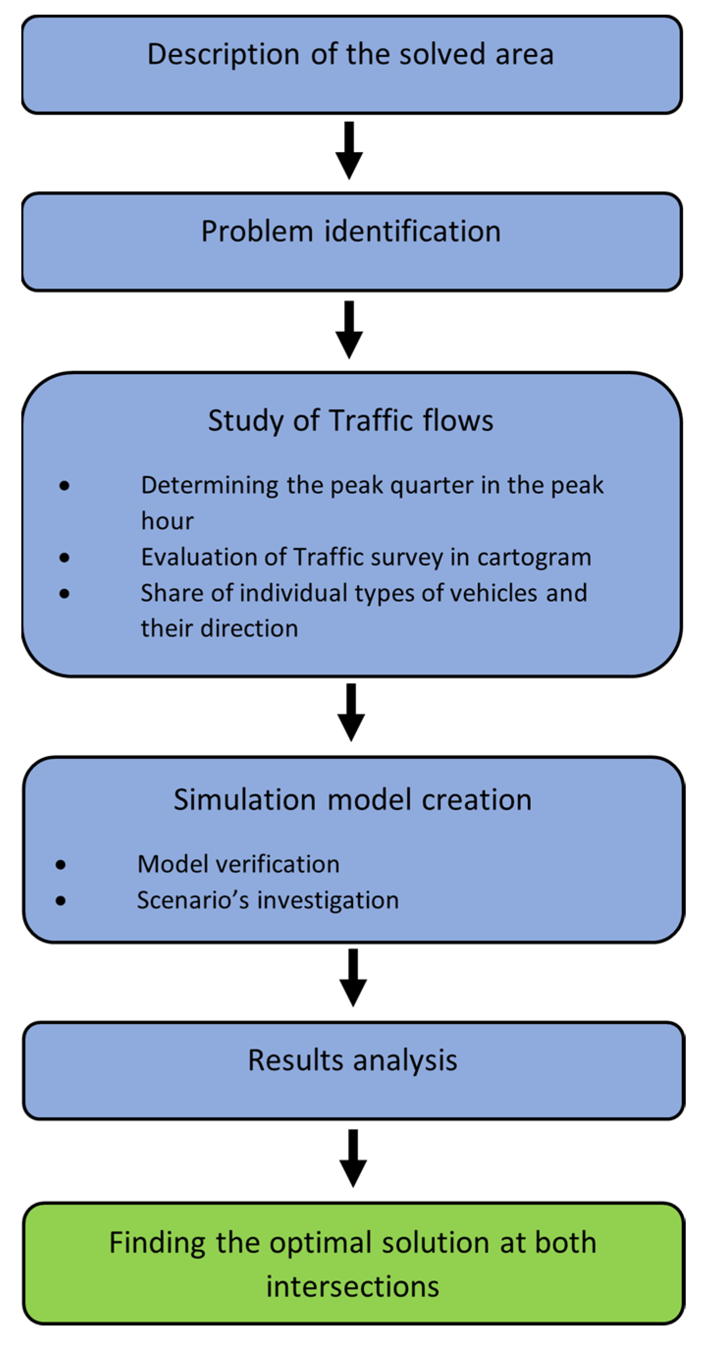
2.2. Research Methodology

This research is based on real observations of two problem crossroads in the city of Kosice. The principle is based on observing traffic flows using real traffic counting at peak times. The aim is to reduce traffic congestion by adjusting signal plans on the monitored section using computer simulation and modelling in ExtendSim8. The research methodology consists of several steps and is briefly described in Figure 2.

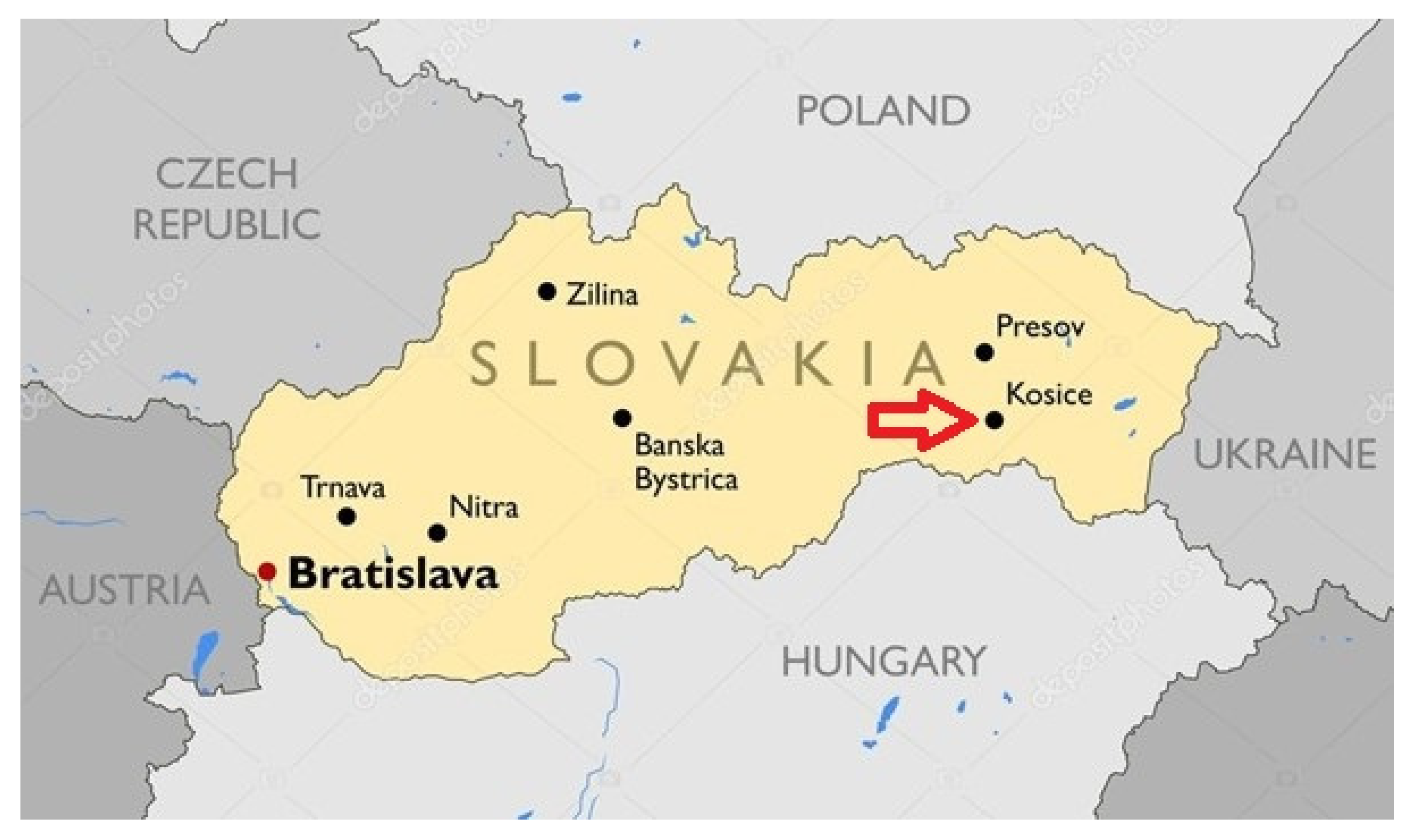
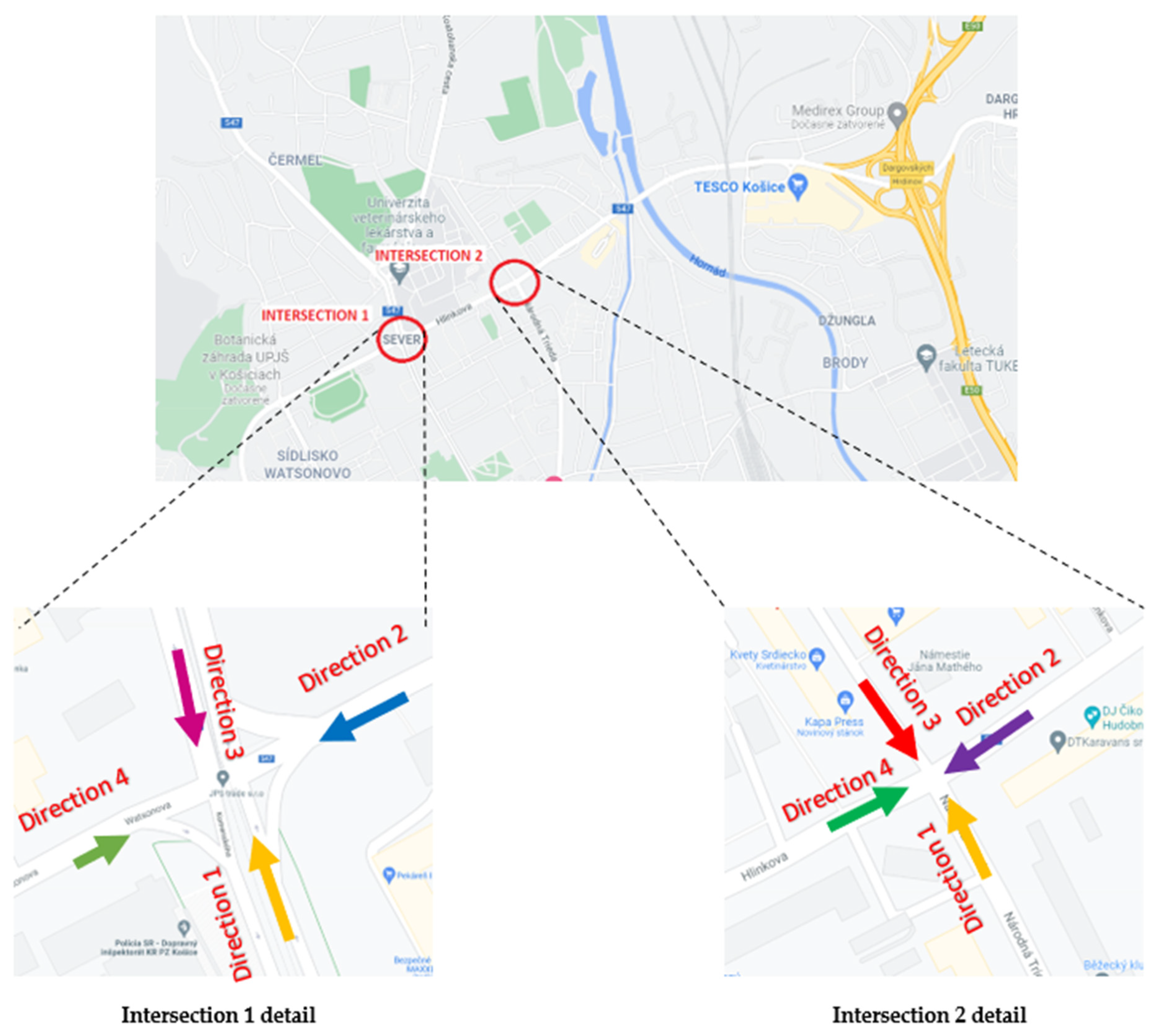
2.3. Description of the Solved Area and Problem Identification

Kosice is the second-largest city in Slovakia. Figure 3 shows the location of the city within the Slovak Republic. Like every major city, the city of Kosice is plagued by congestion caused by high traffic density. In this study, simulations will be created at two intersections; their position can be seen in Figure 4. The lane-setting layout at the investigated intersections is standard. It was not part of the study to change them, as the technical parameters in the site (proximity to buildings, sidewalks, etc.) do not allow it. Near the intersections, there is an exit from the expressway, which puts even more strain on the congested road. The principle of the study is to find the optimal signalling plan for the control of the given intersections using the simulation program ExtendSim 8.

2.4. Study of Traffic Flows on the Researched Intersection with Traffic Lights

Surveys are an irreplaceable need in traffic planning, design and modernization, as well as in the assessment of roads, intersections, etc. To obtain input data for the simulation model, a directional survey was performed at two intersecting intersections. This survey was conducted every working day for two weeks during the morning rush hour, which is from 7:00 to 8:00. The time between 7:00 and 8:00 was chosen based on a preliminary survey, when it was found that at this very hour the traffic intensity is the highest of the whole day and is thus the so-called rush hour. The vehicle data which have been entered in the table are structured according to the respective time, vehicle type and direction of travel. We categorized vehicle types in the composition of cars, trucks, public transport and others. Others are considered, for example, special vehicles, bicycles, motorcycles, etc.

2.4.1. Determining the Peak Quarter in the Peak Hour

For each intersection, a data matrix is created, in which the numbers of vehicles in the categories of passenger cars, trucks and public transport are recorded at 15-min intervals. This is important because passenger cars cross the intersection faster than lorries, not only because of the latter’s slower start-up but also due to the higher weight and length of these vehicles. It is therefore clear that the optimal setting of the signal plan will depend on the proportion of individual vehicles. In

Table 1. Tabular display of the results of the directional survey at intersection 1 in Direction 1 and Direction 2 [veh.].

Matrix 1 Direction 1 (Komenskeho–Juh)						Matrix 2 Direction 2 (Hlinkova)
	Cars	Trucks	Public tr.	Other	Total		Cars	Trucks	Public tr.	Other	Total
7:00–7:15						7:00–7:15
left	20	2	0	0	22	left	95	1	1	0	97
right	23	2	0	0	25	right	9	0	0	0	9
straight	30	0	4	0	34	straight	215	2	4	0	221
total	73	4	4	0	81	total	319	3	5	0	327
7:15–7:30						7:15–7:30
left	17	2	0	0	19	left	104	1	1	0	106
right	33	1	0	0	34	right	11	0	0	0	11
straight	31	0	5	1	37	straight	239	2	5	1	247
total	81	3	5	1	90	total	354	3	6	1	364
7:30–7:45						7:30–7:45
left	25	3	0	0	28	left	113	2	1	0	116
right	35	2	0	0	37	right	14	0	0	0	14
straight	39	1	5	1	46	straight	282	4	6	1	293
total	99	6	5	1	111	total	409	6	7	1	423
7:45– 8:00						7:45–8:00
left	19	2	0	0	21	left	118	1	1	0	120
right	30	1	0	0	31	right	10	0	0	0	10
straight	34	1	4	1	40	straight	266	3	5	1	275
total	83	4	4	1	92	total	394	4	6	1	405

there is a matrix of measured data for the first monitored intersection at streets Komenskeho—Watsononova (Intersection 1) in directions 1 and 2 and in

Table 2. Tabular display of the results of the directional survey at intersection 1 in Direction 3 and Direction 4 [veh.].

Matrix 3 Direction 3 (Komenskeho–Sever)						Matrix 4 Direction 4 (Watsonova)
	Cars	Trucks	Public tr.	Other	Total		Cars	Trucks	Public tr.	Other	Total
7:00–7:15						7:00–7:15
left	25	2	0	0	25	left	59	0	0	0	59
right	34	0	0	0	34	right	11	0	0	0	11
straight	55	0	1	0	56	straight	189	0	3	0	192
total	114	0	1	0	115	total	259	0	3	0	262
7:15–7:30						7:15–7:30
left	24	0	1	0	25	left	65	1	1	0	67
right	39	0	1	0	40	right	15	0	0	0	15
straight	61	1	2	0	64	straight	202	1	5	1	209
total	124	1	4	0	129	total	282	2	6	1	291
7:30–7:45						7:30–7:45
left	32	0	0	1	33	left	75	0	1	0	76
right	47	0	1	0	48	right	22	0	0	0	22
straight	69	1	3	1	74	straight	222	1	6	1	230
total	148	1	4	2	155	total	319	1	7	1	328
7:45–8:00						7:45– 8:00
left	27	0	1	0	28	left	65	0	0	0	65
right	40	0	0	0	40	right	18	0	0	0	18
straight	64	0	3	0	67	straight	219	0	5	0	224
total	131	0	4	0	135	total	302	0	5	0	307

in directions 3 and 4. Intersection diagrams and directions are marked in Figure 4. We proceeded similarly in every direction at the Narodna Trieda—Hlinkova (Intersection 2). In total, there are four matrices for one intersection and, because two intersections are solved, we have 8 matrices. The survey was conducted on a working day for 2 weeks during the morning rush hour. The values in the following tables are based on average survey values. The values in Table 1 and Table 2 present an average number of vehicles in the specified time frame, such as 7:00–7:15, 7:15–7:30, 7:30–7:45 or 7:45–8:00, during the two-week survey.

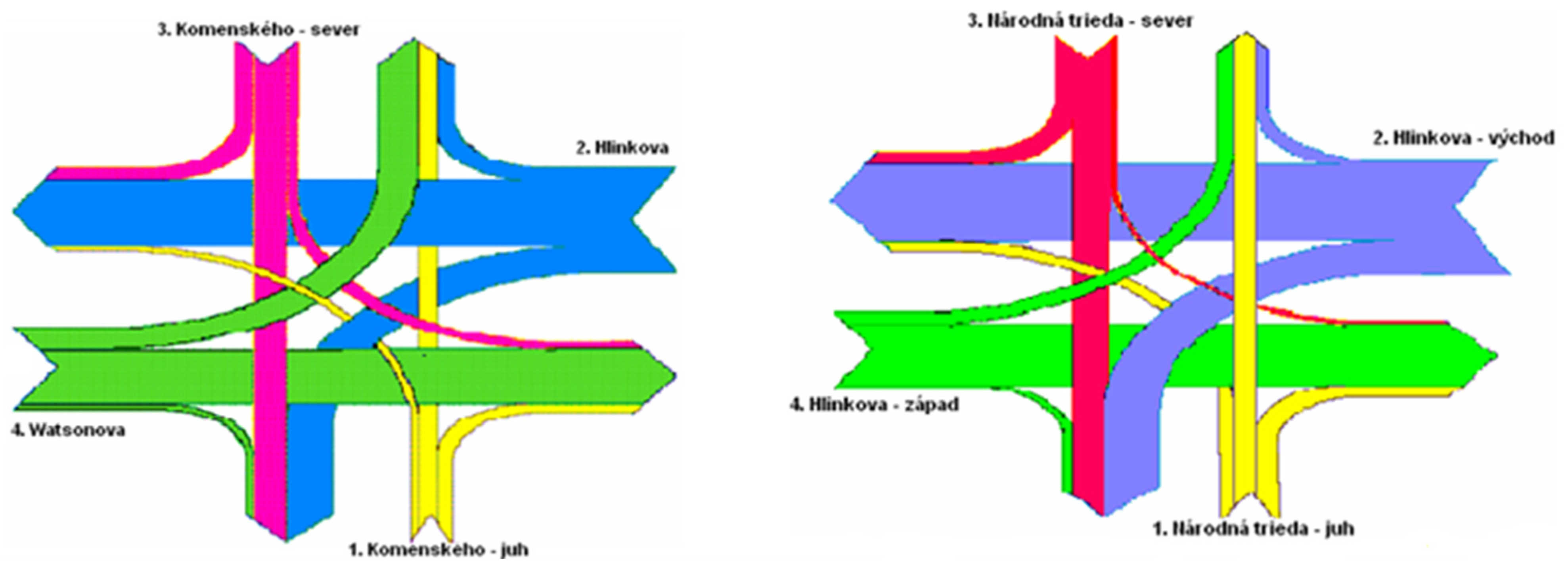
2.4.2. Evaluation of the Traffic Survey in the Cartogram

Based on the measured data, a peak quarter-hour was found, i.e., 15-min interval in which most vehicles passed the intersection. For both measured intersections, the peak quarter-hour was set between 7:30–7:45. The search for the optimal setting of the signal plan using the simulation model will therefore be in this peak quarter.

The cartograms in Figure 5 show the total intensity in the morning at Intersection 1 (Komenskeho—Watsonova) and Intersection 2 (Narodna trieda—Hlinkova).

The most congested directions at Intersection 1 (Komenskeho—Watsonova) are Direction 2 (Hlinkova) and Direction 4 (Watsonova). A total of 2707 vehicles passed there, which is 1799 more vehicles compared to less loaded directions. Less congested directions were Direction 1 (Komenskeho—Juh) and Direction 3 (Komenskeho—Sever), with a total number of vehicles—908 (33.5%).

At Intersection 2 (Narodna trieda—Hlinkova—zapad), the most congested directions are Direction 2 (Hlinkova—vychod) and Direction 4 (Hlinkova—zapad), through which up to 3123 vehicles passed in the monitored period, which is 13% more than in the most congested directions on intersection 1. The less congested directions are Direction 1 (Narodna trieda—juh) and Direction 3 (Narodna trieda—sever).

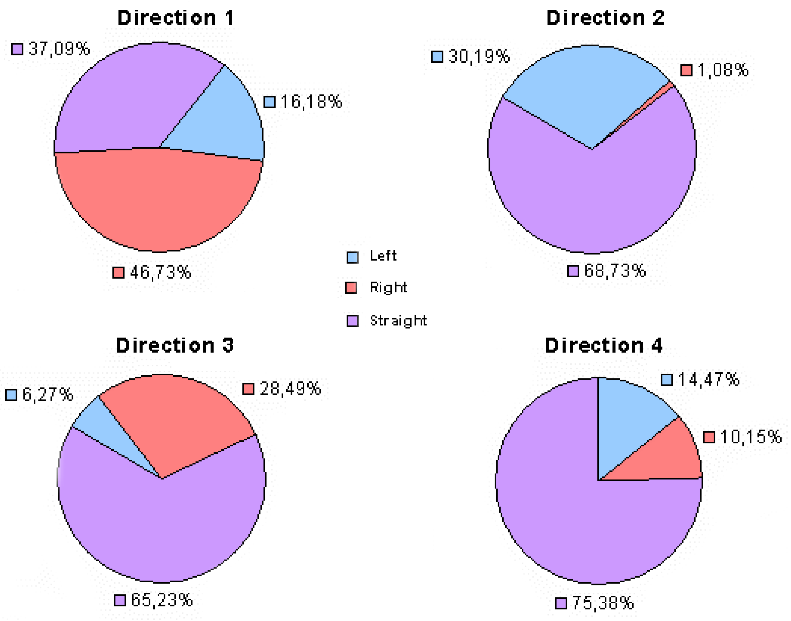
2.4.3. Share of Individual Types of Vehicles and Their Direction

During the survey, vehicles were also recorded by type. The following table (

Table 3. Number of individual types of vehicles at both intersections between 7:00–8:00.

Vehicle Type	Intersection 1		Intersection 2
	Quantity [veh.]	Proportion [%]	Quantity [veh.]	Proportion [%]
cars	3491	96.57	4120	97.37
trucks	38	1.05	42	1.00
public transportation	76	2.10	61	1.44
other	10	0.28	8	0.19
total	3615	100	4231	100

) shows the number as well as the proportion of individual vehicle types that passed intersection 1 in the observed period.

The modal split is important because passenger cars cross the intersection faster than trucks or buses, not only because of the latter’s slow start but also due to the higher weight and length of the vehicle. For example, one truck is 1.5 times a passenger car in terms of the time it takes to cross an intersection. The coefficients in

Table 4. Coefficients of types of vehicles.

Vehicle Type	Coefficient [-]
Car	1.0
Truck	1.5
Public	1.6
Other	1.4

were determined based on our observations at the intersections. It is therefore clear that the optimal setting of the signal plan will depend on the proportion of individual vehicles.

The table shows that passenger vehicles accounted for the largest share, accounting for about 97% of the total number of vehicles crossed. They are followed by public transport vehicles with just over 2.10% at intersection 1 and 1.44% at intersection 2. Trucks make up only about 1% of passing vehicles. The term other vehicles included all other vehicles not belonging to the remaining categories (e.g., bicycles, special motor vehicles and international road transport buses). However, they also accounted for only a small percentage of the total number of vehicles driven, namely 0.28% and 0.19%.

Shares of Individual Driving Directions at the Intersection

From

Table 5. Number of vehicles in each direction at the intersection 1.

Turn Direction	Number of Vehicles from Direction 1 [veh.]	Number of Vehicles from Direction 2 [veh.]	Number of Vehicles from Direction 3 [veh.]	Number of Vehicles from Direction 4 [veh.]
left	90	439	111	267
right	127	44	162	66
straight	374	1136	261	855
total	591	1619	534	1188

it is possible to see how many vehicles turned right, left or crossed the intersection in each direction. Subsequently, Figure 6 shows the proportion of individual driving directions at intersection 1.

In all directions, crossing the intersection prevailed without changing the direction of travel, i.e., straight. Many vehicles in Directions 1 and 3 turned right, and a high percentage in all directions represents the most difficult passage through the intersection: on the left.

The following table (

Table 6. Number of vehicles in each direction at the intersection 2.

Turn Direction	Number of Vehicles from Direction 1 [veh.]	Number of Vehicles from Direction 2 [veh.]	Number of Vehicles from Direction 3 [veh.]	Number of Vehicles from Direction 4 [veh.]
left	89	586	35	171
right	257	21	159	120
straight	204	1334	364	891
total	550	1941	558	1182

) shows the number of vehicles that turned right, left or went through intersection 2 straight. Subsequently, Figure 7 shows the proportion of individual driving directions at intersection 2.

As at intersection 1, most vehicles passed straight at intersection 2. Specific is Direction 1, where most cars turned right, and Direction 2, where cars turned right minimally.

2.4.4. Length of the Control Cycle

The control cycle is the time[s] during which the whole set of signal images takes place on one signal. According to an international agreement concluded in 1969 in Vienna, the order of the signal images on the signal area of a traffic signal is as follows: red, red-yellow, green, yellow, red.

The length of the cycle is given by constant intervals, traffic load, number of phases and the layout of the intersection. When choosing a cycle length, keep in mind that a cycle that is too short reduces the capacity of the intersection, and, conversely, a cycle that is too long can lead to a lack of green phases during which no vehicle passes through the intersection. Long cycles also increase time losses and lead to a decrease in the effective management of intersection traffic lights. The length of the cycle ranges from 20 to 120 s and depends on the number of vehicles entering the intersection, on the way the vehicles turn and their intensity, on the width of the passage and its length and on the construction modifications of the intersection. In our case, the length of the green cycle is 30 s, and we will perform simulations for different lengths of the green cycle in 5-s increments.

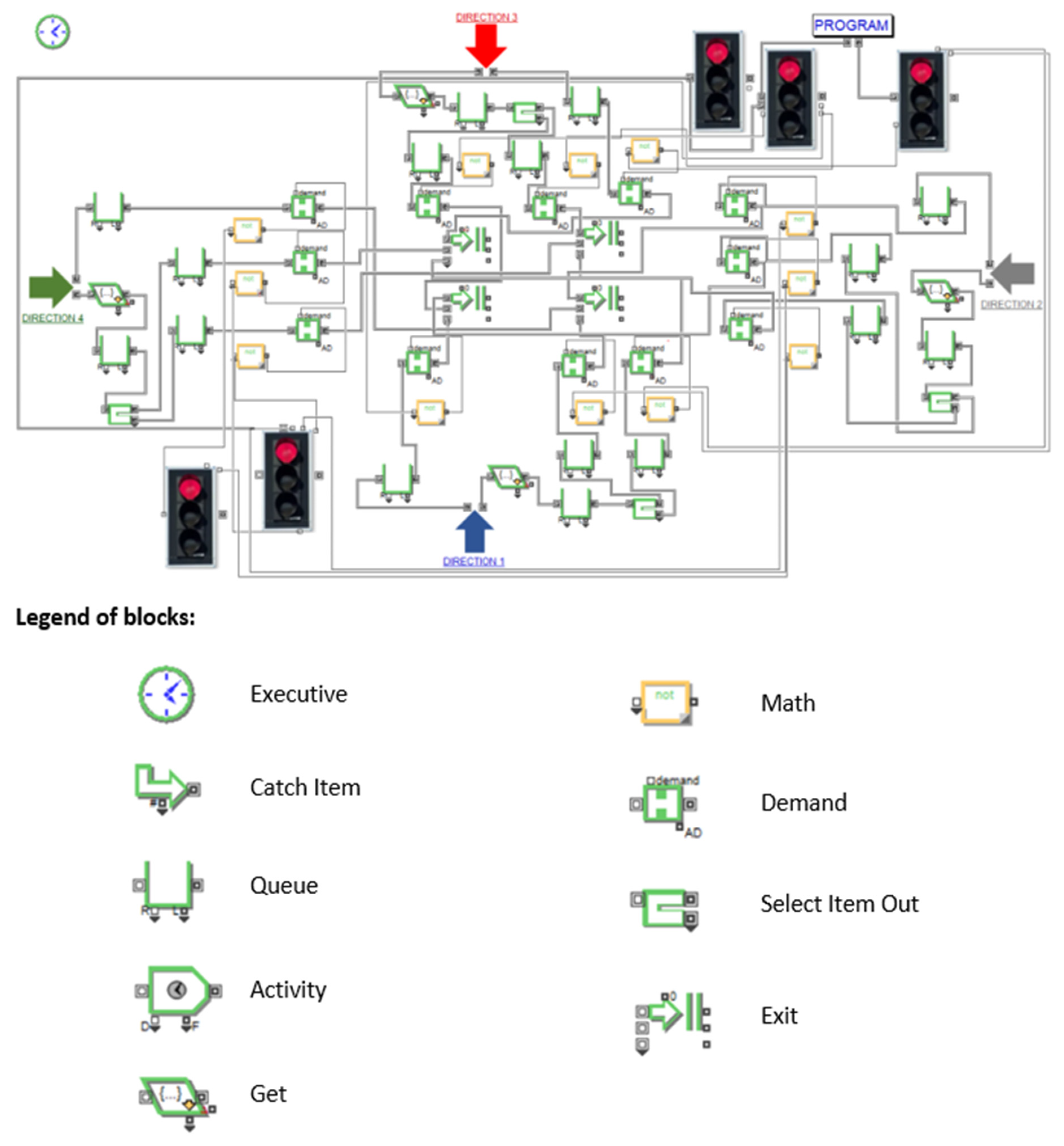
2.5. Simulation Model Creation

By researching the intersection in the previous section, we obtained data that we will now use to create a simulation model of the intersection. The simulation results will only be accurate if we have good input data. The intersection simulation model is created in the ExtendSim8 program.

The simulation consists of blocks that are interconnected and determine the direction of flows (the flow of the passage of vehicles through the intersection). Each block used represents part of a process or operation in a simulation model. The blocks have their unique icon, and the name there expresses their basic use within the model [44,45].

When creating the model, we mainly used blocks from the Item libraries, which is a block library for modelling discrete processes, and Value, which is a block library for modelling continuous processes.

1.

Used blocks from the Item Library:

• Block Executive: forms the heart of every discreet model. Allows the user to control the course of the simulation until the selected end time or until a specified number of events.
• Block Create: used to generate the input of requests to the discrete simulation model; the generation is realized based on the selected type of distribution of the random variable.
• Block Get: displays and outputs the properties of the elements that pass through the block. It is possible to work with multiple features and multiple output connectors.
• Block Select Item Out: chooses which output gets the elements from the input according to a certain decision.
• Block Queue: the block performs the function of a queue in which requests are waiting to be processed. In our case, it works on the principle of First In, First Out.
• Block Gate: limits the number of elements passing through the model; allows you to track how many elements are in which part of the model.
• Block Exit: the block removes processed requests from the simulation model from one input to several. Provides information about the number of requests processed in the dialog box. Additional connectors provide information on the total and a partial number of processed requests, which can be used, for example, to create graphs.

2.

Used blocks from the Value Library:

• Block Math: the block performs various mathematical operations from the input connectors to a single output value on the output connector. The resulting block graphics are also adjusted according to the selected mathematical operation.

Furthermore, various blocks from the Plotter library, which is used for creating graphs, and from the Rate library for evaluating the simulation results were used. Figure 8 shows the created simulation model of Intersection 1. A similar model is also created for Intersection 2.

2.5.1. Model Verification

Before we start working with the model, it is necessary to verify it, i.e., to verify whether the model provides real results. For this reason, the current traffic situation was simulated on the created model, while the results obtained from the simulation model are compared with the real state. After several adjustments, the model was finally fine-tuned.

The verification consists in finding out that all the blocks in the simulation model are correctly connected. The simulation model prepared in this way is ready for experimentation. The experiment with the model is performed by comparing the values that were added in the traffic survey with the values that are generated in the simulation at the beginning of the simulation. In the tables (

Table 7. The difference between the number of vehicles from simulation and from a survey at intersection 1.

Turn Direction	Measured Values from a Survey [veh.]				Simulation Values [veh.]
	Direction 1	Direction 2	Direction 3	Direction 4	Direction 1	Direction 2	Direction 3	Direction 4
left	90	439	111	267	90	439	111	267
right	127	44	162	66	127	44	162	66
straight	374	1136	261	855	374	1136	261	855
total	591	1619	534	1188	591	1619	534	1188

and

Table 8. The difference between the number of vehicles from simulation and from a survey at intersection 2.

Turn Direction	Measured Values from a Survey [veh.]				Simulation Values [veh.]
	Direction 1	Direction 2	Direction 3	Direction 4	Direction 1	Direction 2	Direction 3	Direction 4
left	89	586	35	171	89	586	35	171
right	257	21	159	120	257	21	159	120
straight	204	1334	364	891	204	1334	364	891
total	550	1941	558	1182	550	1941	558	1182

) it is possible to see the difference in the number of vehicles in the directions at both monitored intersections. These tables show that the actual state is identical to the simulation. As a result, the model is verified.

2.5.2. Scenario’s Investigation

The next phase is the creation of model scenarios, which consists in setting the parameters of the model so that the permeability of both intersections is optimal and thus the model as best as possible to be effective. As part of the simulation, four scenarios will be created to improve the permeability at intersection 2, and, subsequently, five scenarios will be created at intersection 1. In total, nine scenarios will be simulated.

We will first simulate at intersection 2, as the direction from Hlinkova street is problematic. At the beginning, the current situation at intersection 2 will be presented as scenario 1. Then we will increase the green signal for 5 s as scenarios 2–4, when we will find out which state is optimal at intersection 2. Then we will simulate the current state at intersection 1 as scenario 5. As scenario 6, the situation at intersection 1 will be simulated at the current length of the green signal at intersection 1 and the change of the green signal at intersection 2 (optimal state at intersection 2). Subsequently, as scenarios 7–9, we will increase the green signal at intersection 1 by 5 s when the green signal at intersection 2 is already changed and is optimal. An overview of the scenarios can be found in

Table 9. Overview of scenarios at both intersections.

Scenario	Change of Green Signal
	At Intersection 1		At Intersection 2
	Green Signal Length [sec.]	The Difference Compared to the Current State [sec.]	Green Signal Length [sec.]	The Difference Compared to the Current State [sec.]
Scenario 1			30	0
Scenario 2			35	+5
Scenario 3			40	+10
Scenario 4			45	+15
Scenario 5	30	0	30	0
Scenario 6	30	0	40	+10
Scenario 7	35	+5	40	+10
Scenario 8	40	+10	40	+10
Scenario 9	45	+15	40	+10

.

3. Results and Discussion

Based on repeated observations at both intersections between 7.00 a.m. and 8.00 a.m., it was found that the critical points of the intersections are Direction 2 (i.e., the whole Hlinkova street from Tesco and expressway exit). The whole street is under the so-called green wave and the duration of the green signal in this direction is 30 s. Figure 9 shows the critical points of the intersections.

At critical points, during the duration of the green signal in other directions, many vehicles accumulate. As mentioned above, the duration of the green signal for critical directions is 30 s, but when it is triggered, not all vehicles will be able to cross the intersections, and long columns begin to form in critical directions. Unfortunately, this fact adversely affects the flow of traffic, which is an important factor in reducing accidents.

In the monitored period, 1941 vehicles passed in intersection 2 (Narodna Trieda—Hlinkova) in the critical direction (Hlinkova), which makes up approximately 68% of the total number of vehicles—2843—that came to the intersection. The remaining 32% of vehicles remained standing in long congestions.

At intersection 1 (Komenskeho—Watsonova), 34% fewer vehicles passed in the critical direction (Hlinkova) during the monitored period than in the critical direction at intersection 2. In total, 1519 vehicles passed in the direction, which makes up 81% of the total number of incoming vehicles.

3.1. Finding the Optimal Solution at an Intersection 2

To determine the optimal solution, a simulation model was used, in which the values obtained by the directional survey were entered. The optimal solution is assumed to be a solution where the maximum number of vehicles cross the intersection and the number of vehicles that remain in front of the intersection is minimal. The simulation showed that the maximum limit of the increase of the green signal at the intersections, so that long columns do not start to form in other directions, is 15 s, i.e., from the current 30 s to max 45 s.

Values from the time interval from 7.30 to 7.45 were used in the simulation model when most vehicles passed through the intersection. If the optimal length of the extension is determined for this time interval, it is obvious that this extension will also be suitable for other, less stressed time intervals.

Figure 10 graphically shows the simulation results for the time window 7.30—7.45, when the number of vehicles at the intersection is the highest. Vehicles that have passed through the intersection are shown by a blue curve, and vehicles that have stood at the intersection are represented by a red curve.

Based on this graph, the optimal solution at intersection 2 is to extend the green signal to 40 s. At that time, the intersection was able to release the maximum number of vehicles, and the number of vehicles left in front of the intersection was significantly reduced.

In

Table 10. Intersection 2 conditions before green signal increase (30 s).

Time Frame	Number of Vehicles that Came to the Intersection [veh.]	Number of Vehicles that Passed the Intersection [veh.]	[%]	Number of Vehicles Standing in front of an Intersection [veh.]	[%]
7.00–7.15	592	434	73	158	27
7.15–7.30	734	497	67	237	33
7.30–7.45	801	517	65	284	35
7.45–8.00	716	493	68	223	32
total	2843	1941		902

,

Table 11. Intersection 2 conditions after increasing the green signal to 35 s.

Time Frame	Number of Vehicles that Came to the Intersection [veh.]	Number of Vehicles that Passed the Intersection [veh.]	[%]	Number of Vehicles Standing in front of an Intersection [veh.]	[%]
7.00–7.15	592		75		25
7.15–7.30	734		68		32
7.30–7.45	801		69		31
7.45–8.00	716		70		30
total	2843

,

Table 12. Intersection 2 conditions after increasing the green signal to 40 s.

Time Frame	Number of Vehicles That Came to the Intersection [veh.]	Number of Vehicles That Passed the Intersection [veh.]	[%]	Number of Vehicles Standing in front of an Intersection [veh.]	[%]
7.00–7.15	592	504	86	88	14
7.15–7.30	734	579	79	155	21
7.30–7.45	801	605	76	196	24
7.45–8.00	716	569	80	147	20
total	2843	2257		586

and

Table 13. Intersection 2 conditions after increasing the green signal to 45 s.

Time Frame	Number of Vehicles that Came to the Intersection [veh.]	Number of Vehicles That Passed the Intersection [veh.]	[%]	Number of Vehicles Standing in front of an Intersection [veh.]	[%]
7.00–7.15	592	444	75	148	25
7.15–7.30	734	499	68	235	32
7.30–7.45	801	593	74	208	26
7.45–8.00	716	501	70	215	30
total	2843	2037		806

, it is possible to see the results of the simulation after increasing the time intervals from the current state of 30 s to the maximum limit of the increase of the green signal as stated above in the text, i.e., 45 s. Thus, four scenarios (scenario 1, scenario 2, scenario 3, scenario 4) were simulated.

Table 10 shows the condition at intersection 2 (Narodna Trieda—Hlinkova) before the increase of the green signal in the critical direction 2 (Hlinkova). The most critical time is (as mentioned above) the time from 7.30 to 7.45, when we had the most vehicles left at the intersection: up to 35% of the total number of vehicles that came to the intersection. We also had the fewest vehicles at that time: only 65%.

Table 12 shows the state at intersection 2 after increasing the length of the green signal from 30 s to 40 s, which is the optimal state. We proceeded similarly when increasing the green signal to 35 and 45 s. The number of vehicles standing in front of the intersection has decreased significantly. Compared to the actual situation, 343 more vehicles passed through it and the number of stationary vehicles in the most critical time (7.30–7.45) decreased by as much as 11%.

Table 11, Table 12 and Table 13 show the simulation results for green signal lengths for 35 and 45 s. As can be seen from the results in Table 13, with the simulated green wave length in direction 35 to 45 s, the number of vehicles passing the intersection starts to decrease gradually, which suggests that increasing the length of the green signal is not appropriate indefinitely, but in the case of this intersection it is 40 s.

The table also shows how many vehicles came to the intersection, how many of them passed and how many vehicles were left standing at the intersection. The number of vehicles is also expressed as a percentage.

As we extended the duration of the green signal by 10 s in the busiest direction at intersection 2, more vehicles passed through the intersection. For us not to start forming long columns at intersection 1 where the traffic was flowing, it iwa necessary to find an optimal solution to increase the duration of the green signal on it as well.

3.2. Finding the Optimal Solution at an Intersection 1

The following graph in Figure 11 shows the evolution of the curves of the vehicles that passed and remained in front of intersection 1 during the change of time intervals.

A simulation model was used to determine the optimal solution, into which the values obtained during the observed period were entered. It can be seen from the graph in Figure 11 that the optimal solution at intersection 1 is to extend the green signal to 35 s. At that time, the intensity of our vehicles increased significantly, by up to 8%. After increasing the length of the green signal to 40 and 45 s, the number of vehicles that passed the intersection increased by only 4%. It is necessary to increase the green signal in the critical direction by 5 s for the efficient operation of the intersection. At intersection 1 we will simulate 5 scenarios (Scenario 5, Scenario 6, Scenario 7, Scenario 8, Scenario 9).

Table 14. Intersection 1 condition before the green signal increase (30 s).

Time Frame	Number of Vehicles That Came to the Intersection [veh.]	Number of Vehicles That Passed the Intersection [veh.]	[%]	Number of Vehicles Standing in front of An Intersection [veh.]	[%]
7.00–7.15	381	327	86	54	14
7.15–7.30	443	364	83	79	17
7.30–7.45	549	423	78	126	22
7.45–8.00	503	405	81	98	19
total	1876	1519		357

shows the situation at intersection 1 (Komenskeho—Watsonova) before the increase of the green signal in Direction 2. The number of vehicles that came to the intersection is 44% less than at intersection 2. It is also the most critical time from 7.30 to 7.45, when most vehicles remained standing at the intersection: up to 22% of the total number of vehicles that came to the intersection.

In the next table (

Table 15. Intersection 2 conditions after increasing the green signal at intersection 1 to 40 s while intersection 1 has 30 s.

Time Frame	Number of Vehicles that Came to the Intersection [veh.]	Number of Vehicles That Passed the Intersection [veh.]	[%]	Number of Vehicles Standing in front of an Intersection [veh.]	[%]
7.00–7.15	428	327	77	101	23
7.15–7.30	498	364	74	134	26
7.30–7.45	625	423	68	202	32
7.45–8.00	568	405	72	163	28
total	2119	1519		600

) we will show how the conditions at intersection 1 change due to the change in the length of the green signal at intersection 2 (Section 3.1). Recall that at intersection 2, the length of the green signal increased from the original 30 s to 40 s when the number of vehicles that passed the intersection was the highest. By increasing the duration of the green signal by 10 s at intersection 2, we received 12% more vehicles at intersection 1, which had an adverse effect on the number of vehicles left standing at the intersection. In the most critical time, 7.30–7.45, the number of vehicles standing in front of the intersection increased by up to 10% (see Table 15).

Due to the increase in the number of vehicles in front of the intersection, the duration of the green signal at intersection 1 was increased from 30 s to 35 s (

Table 16. Condition at intersection 1 after increasing the green signal to 35 s.

Time Frame	Number of Vehicles That Came to the Intersection [veh.]	Number of Vehicles That Passed the Intersection [veh.]	[%]	Number of Vehicles Standing in front of an Intersection [veh.]	[%]
7.00–7.15	428	374	87	54	13
7.15–7.30	498	412	83	86	17
7.30–7.45	625	499	80	126	20
7.45–8.00	568	460	81	108	19
total	2119	1745		374

). Details can be seen in Table 16. Then, 10% more vehicles passed through the intersection and the number of vehicles standing in front of the intersection thus decreased by 8%.

We proceeded similarly when increasing the green signal to 40 and 45 s (

Table 17. Condition at intersection 1 after increasing the green signal to 40 s.

Time Frame	Number of Vehicles That Came to the Intersection [veh.]	Number of Vehicles That Passed the Intersection [veh.]	[%]	Number of Vehicles Standing in front of an Intersection [veh.]	[%]
7.00–7.15	428	370	86	58	14
7.15–7.30	498	403	81	95	19
7.30–7.45	625	481	77	144	23
7.45–8.00	568	454	80	114	20
total	2119	1708		411

and

Table 18. Condition at intersection 1 after increasing the green signal to 45 s.

Time Frame	Number of Vehicles That Came to the Intersection [veh.]	Number of Vehicles That Passed the In-tersection [veh.]	[%]	Number of Vehicles Standing in front of an Intersection [veh.]	[%]
7.00–7.15	428	359	84	69	16
7.15–7.30	498	406	82	92	18
7.30–7.45	625	474	76	151	24
7.45–8.00	568	453	80	115	20
total	2119	1692		427

). As can be seen from the results in Table 18, with the simulated green wave length in direction 1 40 s, the number of vehicles passing the intersection begins to decrease gradually, suggesting that increasing the length of the green signal is not appropriate indefinitely but in the case of this intersection it is 40 s.

4. Conclusions

In the article, the signal plan of two intersections at a critical section in the city of Kosice was optimized using the ExtendSim simulation program. The aim was to find the right setting for the length of the green signal in the busiest direction of Hlinkova Street (in our case direction 2), where there are 2 intersections and where there are frequent congestions and accidents. From the point of view of the solution, the most advantageous length of the green signal is that at which the largest number of cars passes through the intersection and at the same time the smallest possible number of cars remains standing at the intersection. The results show that the optimal setting of the length of the green signal in direction 2 at intersection 1 is 40 s, while at the next intersection, which in this study we refer to as intersection 2, the optimal setting of the length of the green signal is 35 s.

The duration of the green signal was increased to 35 and 40 s due to the improvement of fluidity and thus also the reduction of accidents. After this increase, 173 more vehicles passed through intersection 1, and at intersection 2, the number of vehicles standing in front of the intersection decreased by 316 vehicles.

In almost all published scientific studies, one of the available pieces of specialized software such as PTV Vissim, Aimsun, etc. is used to simulate intersections. Although these programs are state-of-the-art in modeling and simulating traffic or intersections, not everyone has access to them. In this article, we therefore decided to introduce the universal simulation tool ExtendSim, which is preferably used for continuous and discrete simulation, especially in manufacturing plants or warehouses, but has not yet been used in any known publication to simulate transport problems. The article points out that a universal simulation program such as ExtendSim can also be used in the design or assessment of signal plans at intersections. The study aimed to find the optimal solution that would improve the permeability of intersections. To improve the situation at the intersections, a simulation model was used, in which the values obtained by the directional survey were entered. The simulation results showed an optimal green signal extension.

Another point of the research was to point out that many simulation programs such as Aimsun and PTV Vissim are currently in use, which creates a very high-quality simulation. However, these programs are very expensive; in addition, in several studies, only the student version is used (for financial reasons). This problem is not only present in Slovakia but also in other countries. Not all tools are available in student versions, simulations are often inaccurate and their results are inaccurate. With this study, we wanted to show that even general simulation software can create quality simulations, and thus to motivate other researchers and Ph.D. students to use this software. Open source simulation software such as MatSim is specially designed for traffic flow simulation, while the ExtenSim is not. Therefore, we consider it very beneficial to adapt the ExtendSim software, which is used in many academic institutions across the country for traffic intersection simulation. The ExtendSim8 simulation program has not yet been used in any scientific study to optimize intersection lighting plans. Setting up signaling plans in ExtendSim8 is relatively simple and fast, allowing the user to perform paremtric studies in a short time. On the other hand, the PTV Vissim program is very user-friendly and graphically intuitive, but changing signal plans is quite difficult. The big advantage of ExtendSim8 is that the parameters and logic of the model can be changed “at runtime”, and there is no need to wait for the end of the simulation.

The following research studies will focus on the creation of simulation models for other types of intersections and will also implement other participants crossing the intersections, namely pedestrians, cyclists and trams, which were not part of this research.

With the use of universal simulation software tools, traffic signal timing plans can be optimized by enhancing traffic efficiency and safety. Traffic safety is one of the most important positive consequences of optimizing signal plans. Therefore, one of the possible directions of future research will be a focus on traffic safety, e.g., using self-learning, adaptive traffic signal control algorithms.

The next point of the future direction of research will be the use of other simulation programs and the creation of a safe real experiment at intersections. The results of experiments performed on the created models will be analysed and compared. This will find out the advantages and disadvantages of the created models.

References

1. Li, J.-Q.; Wu, G.; Zou, N. Investigation of the impacts of signal timing on vehicle emissions at an isolated intersection. Transp. Res. Part D Transp. Environ. 2011, 16, 409–414. [Google Scholar] [CrossRef]
2. Hewage, K.N.; Ruwanpura, J.Y. Optimization of traffic signal light timing using simulation. In Proceedings of the 2004 Winter Simulation Conference, Washington, DC, USA, 5–8 December 2004; Volume 2, pp. 1428–1433. [Google Scholar] [CrossRef]
3. Webster, F.V. Traffic Signal Settings; Road Research Technical Paper; H.M. Stationery Office: London, UK, 1958. [Google Scholar]
4. Ohno, K.; Mine, H. Optimal traffic signal settings—I. Criterion for undersaturation of a signalized intersection and optimal signal setting. Transp. Res. 1973, 7, 243–267. [Google Scholar] [CrossRef]
5. Ohno, K.; Mine, H. Optimal traffic signal settings—II. A refinement of Webster’s method. Transp. Res. 1973, 7, 269–292. [Google Scholar] [CrossRef]
6. Laguna, A.; Rakha, H.; Du, J. Optimizing Isolated Traffic Signal Timing Considering Energy and Environmental Impacts. In Proceedings of the 95th Annual Meeting of the Transportation Research Board, Washington, DC, USA, 10–14 January 2016. [Google Scholar]
7. Köhler, E.; Strehler, M. Traffic Signal Optimization: Combining Static and Dynamic Models. Transp. Sci. 2018, 53, 21–41. [Google Scholar] [CrossRef] [Green Version]
8. Yao, R.; Zhou, H.; Ge, Y.E. Optimizing signal phase plan, green splits and lane length for isolated signalized intersections. Transport 2018, 33, 520–535. [Google Scholar] [CrossRef] [Green Version]
9. Chow, A.; Sha, R.; Li, S. Centralised and decentralised signal timing optimisation approaches for network traffic control. Transp. Res. Procedia 2019, 38, 222–241. [Google Scholar] [CrossRef]
10. Ma, X.; Jin, J.; Lei, W. Multi-criteria analysis of optimal signal plans using microscopic traffic models. Transp. Res. Part D Transp. Environ. 2014, 32, 1–14. [Google Scholar] [CrossRef] [Green Version]
11. Lan, C.-J.; Gu, X. Multi-Criteria Signal Timing Control for Over-Saturated Intersections. IFAC Proc. Vol. 2003, 36, 49–54. [Google Scholar] [CrossRef]
12. Stevanovic, A.; Stevanovic, J.; So, J.; Ostojic, M. Multi-criteria optimization of traffic signals: Mobility, safety, and environment. Transp. Res. Part C Emerg. Technol. 2015, 55, 46–68. [Google Scholar] [CrossRef] [Green Version]
13. Andrejiova, M.; Grincova, A.; Marasova, D.; Grendel, P. Multicriterial assessment of the raw material transport. ACTA Montan. SLOVACA 2015, 20, 26–32. [Google Scholar]
14. Essa, M.; Sayed, T. Self-learning adaptive traffic signal control for real-time safety optimization. Accid. Anal. Prev. 2020, 146, 105713. [Google Scholar] [CrossRef] [PubMed]
15. Reyad, P.; Sayed, T.; Essa, M.; Zheng, L. Real-Time Crash-Risk Optimization at Signalized Intersections. Transp. Res. Rec. 2021, 1–19. [Google Scholar] [CrossRef]
16. Gomes, G.; Gan, Q.; Bayen, A. A methodology for evaluating the performance of model-based traffic prediction systems. Transp. Res. Part C Emerg. Technol. 2018, 96, 160–169. [Google Scholar] [CrossRef]
17. Caliendo, C.; Russo, I.; Genovese, G. Resilience Assessment of a Twin-Tube Motorway Tunnel in the Event of a Traffic Accident or Fire in a Tube. Appl. Sci. 2022, 12, 513. [Google Scholar] [CrossRef]
18. Straka, M.; Lenort, R.; Khouri, S.; Feliks, J. Design of large-scale logistics systems using computer simulation hierarchic structure. Int. J. Simul. Model. 2018, 17, 105–118. [Google Scholar] [CrossRef]
19. Vilarinho, C.; Soares, G.; Macedo, J.; Tavares, J.; Rossetti, R. Capability-enhanced AIMSUN with Real-time Signal Timing Control. Procedia-Soc. Behav. Sci. 2014, 111, 262–271. [Google Scholar] [CrossRef] [Green Version]
20. Maduranga, K.L.D.; Yasamali, R.G.N.; Sathyaprasad, I.M.S.; Weerakoon, H.U. Selection of Optimum Junction Operation Strategy for Gatambe Intersection Using VISSIM Simulation. In Lecture Notes in Civil Engineering; Springer: Singapore, 2020. [Google Scholar] [CrossRef]
21. Boroiu, A.; Neagu, E.; Boroiu, A.; Pârlac, S. Study of the Possibilities to Improve the Service Level of Traffic Light Intersections by Road Traffic Micro-simulation. In SIAR International Congress of Automotive and Transport Engineering: Science and Management of Automotive and Transportation Engineering; Springer: Cham, Switzerland, 2020; pp. 349–358. ISBN 978-3-030-32563-3. [Google Scholar] [CrossRef]
22. Arliansyah, J.; Bawono, R.T. Study on Performance of Intersection Around The Underpass Using Micro Simulation Program. IOP Conf. Ser. Earth Environ. Sci. 2018, 124, 12014. [Google Scholar] [CrossRef]
23. Ahmad Yousef, K.M.; Shatnawi, A.; Latayfeh, M. Intelligent traffic light scheduling technique using calendar-based history information. Futur. Gener. Comput. Syst. 2019, 91, 124–135. [Google Scholar] [CrossRef]
24. Kühnel, N.; Thunig, T.; Nagel, K. Implementing an adaptive traffic signal control algorithm in an agent-based transport simulation. Procedia Comput. Sci. 2018, 130, 894–899. [Google Scholar] [CrossRef]
25. Behrisch, M.; Bieker, L.; Erdmann, J.; Krajzewicz, D. SUMO—Simulation of Urban MObility. In Proceedings of the SIMUL 2011, The Third International Conference on Advances in System Simulation, Barcelona, Spain, 23–28 October 2011. [Google Scholar]
26. Van Haare Heijmeijer, A.; Vaz Alves, G. Development of a Middleware between SUMO simulation tool and JaCaMo framework. ADCAIJ Adv. Distrib. Comput. Artif. Intell. J. 2018, 7, 5–15. [Google Scholar] [CrossRef] [Green Version]
27. Akhter, S.; Ahsan, M.N.; Quaderi, S.J.S.; Al Forhad, M.A.; Sumit, S.H.; Rahman, M.R. A SUMO Based Simulation Framework for Intelligent Traffic Management System. J. Traffic Logist. Eng. 2020, 8, 1–5. [Google Scholar] [CrossRef]
28. Lopez, P.A.; Behrisch, M.; Bieker-Walz, L.; Erdmann, J.; Flotterod, Y.P.; Hilbrich, R.; Lucken, L.; Rummel, J.; Wagner, P.; Wiebner, E. Microscopic Traffic Simulation using SUMO. In Proceedings of the IEEE Conference on Intelligent Transportation Systems, Maui, HI, USA, 4–7 November 2018. [Google Scholar] [CrossRef] [Green Version]
29. Maiorov, E.R.; Ludan, I.R.; Motta, J.D.; Saprykin, O.N. Developing a microscopic city model in SUMO simulation system. J. Phys. Conf. Ser. 2019, 1368, 042081. [Google Scholar] [CrossRef]
30. Ismail, A.; Latif, M.; Awai, M. Exploiting witness for traffic simulation. J. Manag. Sci. 2014, 1, 12–24. [Google Scholar] [CrossRef]
31. Simulation|ExtendSim Simulation Software. Available online: https://extendsim.com/solutions/simulation (accessed on 23 May 2020).
32. Dui, H.; Zheng, X.; Chen, L.; Wang, Z. Model and simulation analysis for the reliability of the transportation network. J. Simul. 2020, 1–10. [Google Scholar] [CrossRef]
33. Pekarcíková, M.; Trebuna, P.; Kliment, M.; Král, S.; Dic, M. Modelling and simulation the value stream mapping—case study. Manag. Prod. Eng. Rev. 2021, 12, 107–114. [Google Scholar] [CrossRef]
34. Pekarcikova, M.; Trebuna, P.; Kliment, M.; Dic, M. Solution of bottlenecks in the logistics flow by applying the kanban module in the tecnomatix plant simulation software. Sustainability 2021, 13, 7989. [Google Scholar] [CrossRef]
35. Bindzar, P.; Saderova, J.; Sofranko, M.; Kacmary, P.; Brodny, J.; Tutak, M. A case study: Simulation traffic model as a tool to assess one-way vs. two-way traffic on urban roads around the city center. Appl. Sci. 2021, 11, 5018. [Google Scholar] [CrossRef]
36. Moll, S.; López, G.; García, A. Analysis of the influence of sport cyclists on narrow two-lane rural roads using instrumented bicycles and microsimulation. Sustainability 2021, 13, 1235. [Google Scholar] [CrossRef]
37. Siroky, J.; Nachtigall, P.; Tischer, E.; Gasparik, J. Simulation of Railway Lines with a Simplified Interlocking System. Sustainability 2021, 13, 1394. [Google Scholar] [CrossRef]
38. Tischer, E.; Nachtigall, P.; Siroky, J. The use of simulation modelling for determining the capacity of railway lines in the Czech conditions. OPEN Eng. 2020, 10, 224–231. [Google Scholar] [CrossRef] [Green Version]
39. Straka, M.; Saderova, J.; Bindzar, P.; Malkus, T.; Lis, M. Computer simulation as a means of efficiency of transport processes of raw materials in relation to a cargo rail terminal: A case study. ACTA Montan. SLOVACA 2019, 24, 307–317. [Google Scholar]
40. Thunig, T.; Scheffler, R.; Strehler, M.; Nagel, K. Optimization and simulation of fixed-time traffic signal control in real-world applications. Procedia Comput. Sci. 2019, 151, 826–833. [Google Scholar] [CrossRef]
41. Paholok, I. Simulácia ako vedecká metóda. Electron. J. Philos. 2008, 2, 1–19. [Google Scholar]
42. Lynx_v Slovensko Mapa—Stocková Ilustrace. Available online: https://cz.depositphotos.com/70380129/stock-illustration-slovakia-map.html (accessed on 4 January 2022).
43. Maps, G. Košice. Available online: https://www.google.com/maps/@48.7380899,21.2482184,14.91z (accessed on 4 January 2022).
44. Behun, M.; Kascak, P.; Hrabcak, M.; Behunova, A.; Knapcikova, L.; Sofranko, M. Investigation of sustainable geopolymer composite using automatic identification technology. Sustainability 2020, 12, 6377. [Google Scholar] [CrossRef]
45. Saderova, J.; Rosova, A.; Behunova, A.; Behun, M.; Sofranko, M.; Khouri, S. Case study: The simulation modelling of selected activity in a warehouse operation. Wirel. Netw. 2021, 28, 431–440. [Google Scholar] [CrossRef]
Figure 1. Relation of simulation to other methods [41].
Sustainability 14 02079 g001
Figure 2. Research methodology.
Sustainability 14 02079 g002
Figure 3. Location of the city of Kosice within the Slovak Republic [42].
Sustainability 14 02079 g003
Figure 4. Location of intersections within Kosice [43].
Sustainability 14 02079 g004
Figure 5. Intersection cartograms (Intersection 1 left, Intersection 2 right).
Sustainability 14 02079 g005
Figure 6. The proportion of individual driving directions at intersection 1.
Sustainability 14 02079 g006
Figure 7. The proportion of individual driving directions at the intersection 2.
Sustainability 14 02079 g007
Figure 8. Simulation model of the intersection 1 in ExtendSim8 program.
Sustainability 14 02079 g008
Figure 9. Critical points of intersections.
Sustainability 14 02079 g009
Figure 10. Number of vehicles that passed and remained standing at intersection 2 within time frame 7.30–7.45.
Sustainability 14 02079 g010
Figure 11. Number of vehicles that passed and remained standing at intersection 1 within time frame 7.30–7.45.
Sustainability 14 02079 g011