
Walkability Compass—A Space Syntax Solution for Comparative Studies


 ,
,  , and
, and
Abstract
:1. Introduction
1.1. Walkability Understanding
1.2. Explaining Walkability with Space Syntax
1.2.1. Space Syntax as Background Theory
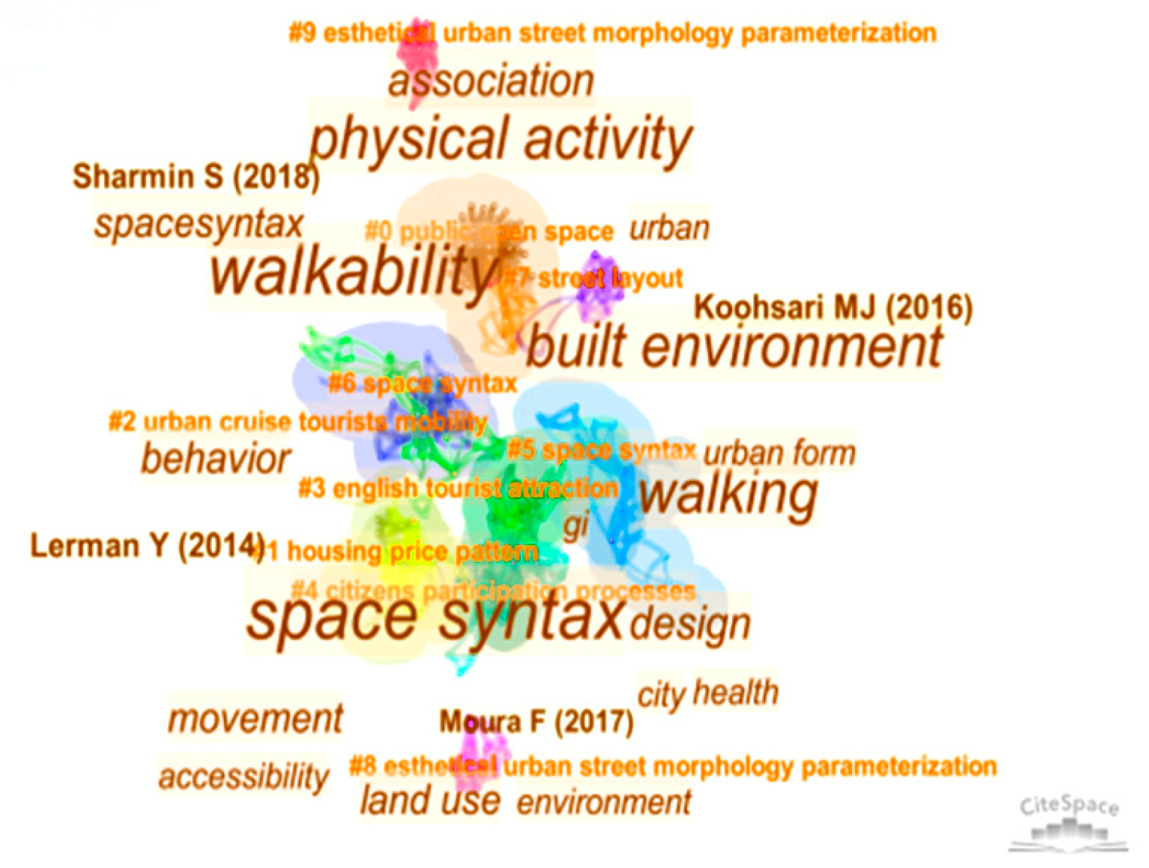
1.2.2. The Growing Interest in Space Syntax Application into Walkability Studies—A Systematic Literature Review
2. Method
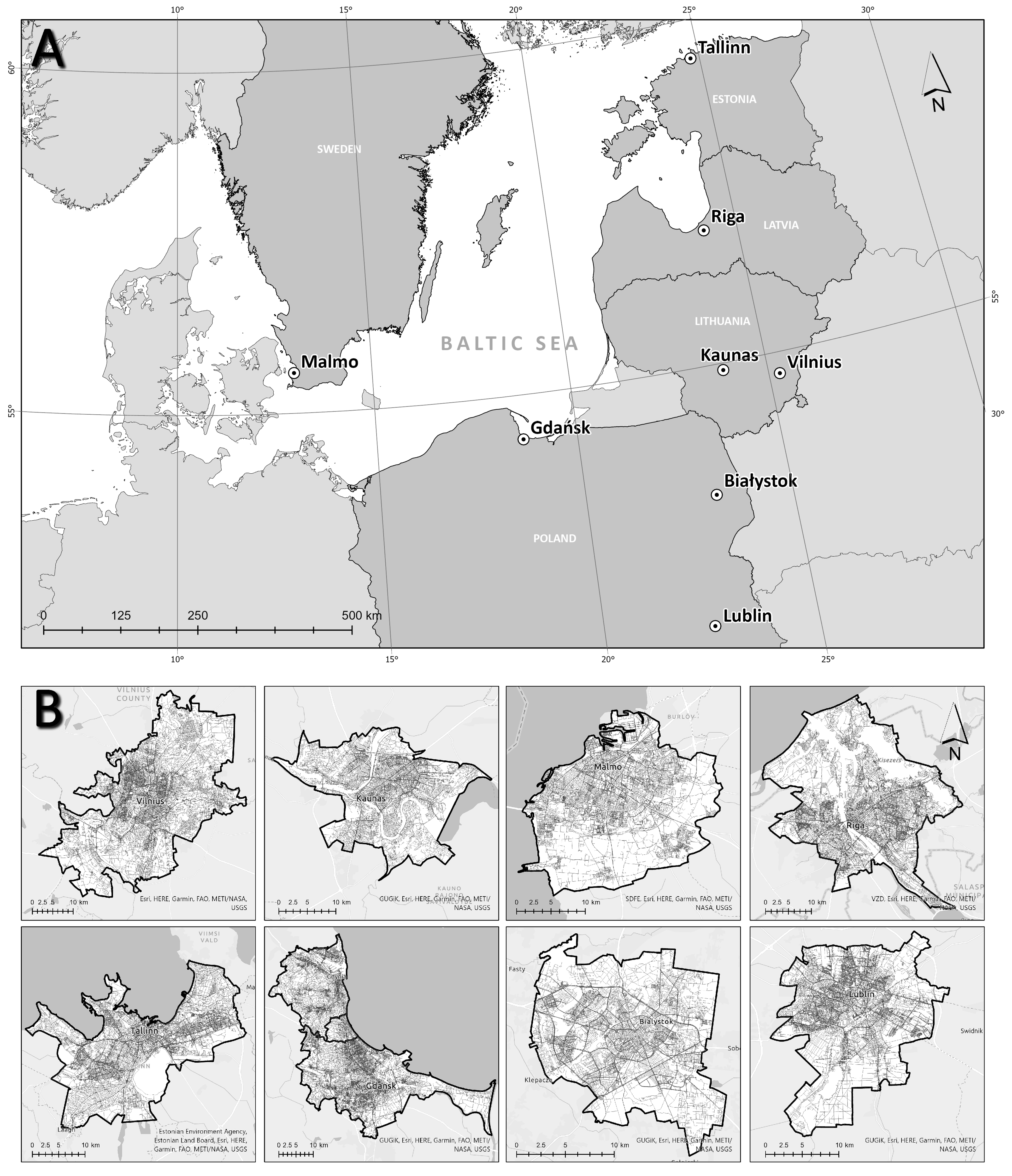
2.1. The Case Study Cities Description
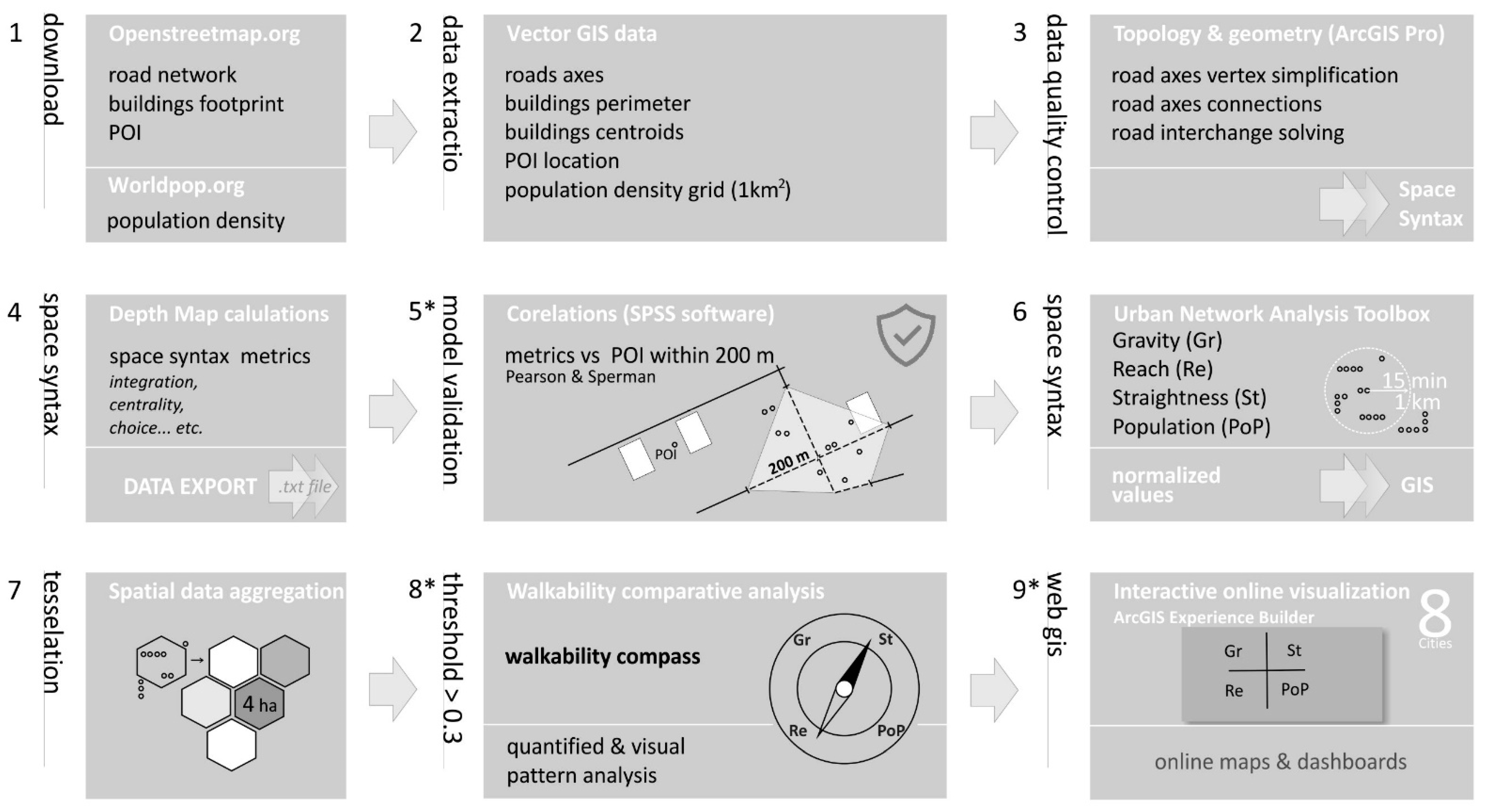
2.2. The Research Method
2.2.1. Open Geospatial Data Management Method (Steps 1–3)
2.2.2. Space Syntax Calculations Method (Steps 4–6)
- Angular segment choice or betweenness centrality, which identifies the probable axes of transit within various radiuses and is calculated as a sum of simulated journeys according to the shortest paths between nodes;
- Angular segment integration or closeness centrality, which identifies the possible zones of attraction or urban centres within various radiuses; it is calculated as reciprocal to a sum of distances between the nodes multiplied by a segment number in Space Syntax Segment analysis;
- Metric segment choice within a radius of 1000 m differs from angular segment choice in how the shortest path is found: it is based on measured distances instead of a sum of angles of the turns on the path. According to Hillier [56], metric distances reflect pedestrian behaviour better in some cases;
- Metric reach within the radius of 1000 m as the length of the reachable street network;
- The total metric depth of 1000 as a sum of distances between nodes while distance is calculated in meters;
- Node count as several nodes/street segments within selected radiuses;
- Angular segment total depth as a sum of distances between nodes while distance is calculated in angles of turns.
2.2.3. Walkability Compass, Pattern and WebGIS Sharing Method (Steps 7–9)
3. Results
3.1. Model Validation Results
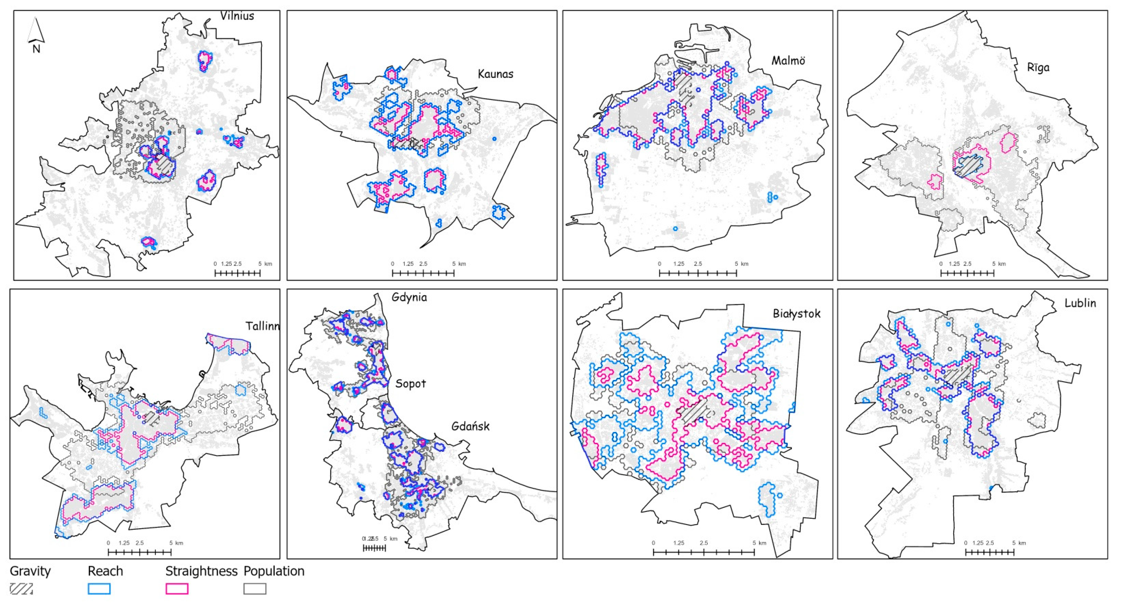
3.2. Walkability Patterns Analysis Results
- Linear—where the majority of an investigated urban phenomenon are allocated along a clear line possibly influenced by a not-evenly-dispersed transport network.
- Hierarchical—with a clear centre and smaller “islands” clustered around it, possibly caused by relatively even transport networks and perhaps longer evolution of the urban network.
- Clusters—made of more or less “even islands”, which depend on some local resources, e.g., specific spatial configurations, accessibility to distinctive landscapes.
- Sectoral—which combines concentric features as clearly expressed, but not dominating the centre, semi-concentric rings of lower intensity around it and dominant corridors—linear centres. Such patterns usually appear because of not-so-evenly spread but concentric street networks and possibly positive and negative synergies between phenomena considered while identifying patterns.
- A multi-nuclei pattern of autonomous islands does not demonstrate the clear presence of the centre. Instead, this pattern indicates the specialisation of territories related to car-oriented street networks where local neighbourhoods do not make a continuous urban background, various social media, and decreased social importance of public spaces.
- Concentric—probably based on a clear multifunctional centre, the radial street network around it and more or less isolated islands at the periphery. The periphery of isolated islands could be seen as a potential continuing outer ring of this pattern in the future.
- The dispersal pattern represents little controlled sprawls of the modelled activities and could be related to car dominance, extensive use of territories and lost spatial synergies.
3.3. The Walkability Compass
3.4. The WebGIS Solution for Cities Walkability Comparison
4. Discussion
5. Conclusions
Author Contributions
Funding
Institutional Review Board Statement
Informed Consent Statement
Data Availability Statement
Acknowledgments
Conflicts of Interest
References
- Loo, B.Y.P. Walking towards a happy city. J. Transport. Geogr. 2021, 93, 103078. [Google Scholar] [CrossRef]
- Kato, H.; Takizawa, A. Which Residential Clusters of Walkability Affect Future Population from the Perspective of Real Estate Prices in the Osaka Metropolitan Area? Sustainability 2021, 13, 13413. [Google Scholar] [CrossRef]
- Jenks, M.; Burton, E.; Williams, K. The Compact City. A Sustainable Urban Form? E. & FN Spon: New York, NY, USA, 1996. [Google Scholar]
- Bettignies, Y.; Meirelles, J.; Fernandez, G.; Meinherz, F.; Hoekman, P.; Bouillard, P.; Athanassiadis, A. The Scale-Dependent Behaviour of Cities: A Cross-Cities Multiscale Driver Analysis of Urban Energy Use. Sustainability 2019, 11, 3246. [Google Scholar] [CrossRef] [Green Version]
- Bolgar, B. Planning for Walkability and Mixed Use. Walkability and Mixed Use. Making Valuable and Healthy Communities. The Prince’s Foundation. 2020. Available online: https://princes-foundation.org/journal/walkability-report (accessed on 20 December 2021).
- de Courrèges, A.; Occelli, F.; Muntaner, M.; Amouyel, P.; Meirhaeghe, A.; Dauchet, L. The relationship between neighborhood walkability and cardiovascular risk factors in northern France. Sci. Total Environ. 2021, 772, 144877. [Google Scholar] [CrossRef] [PubMed]
- Leslie, E.; Butterworth, I.; Edwards, M. Measuring the walkability of local communities using Geographic Information Systems data. In Proceedings of the Walk21-VII, the Next Steps, 7th International Conference on Walking and Liveable Communities, Melbourne, Australia, 23–25 October 2006; Volume 6. [Google Scholar]
- Kato, H.; Kanki, K. Development of walkability indicator for visualising smart shrinking—A case study of sprawl areas in North Osaka Metropolitan Region. Int. Rev. Spat. Plan. Sustain. Dev. 2020, 8, 39–58. [Google Scholar]
- Clark, G. The educational value of the rural trail: A short walk in the Lancashire countryside. J. Geogr. High. Educ. 1997, 21, 349–362. [Google Scholar] [CrossRef]
- Paniagua, A. The hidden life of the historical system of rural roads in a sector of the Guadarrama mountains, Central Spain. Adv. Appl. Sociol. 2020, 10, 257–277. [Google Scholar] [CrossRef]
- Forsyth, A. What is a Walkable Place? The Walkability Debate in Urban Design. Urban. Des. Int. 2015, 20, 274–292. [Google Scholar] [CrossRef]
- Hillier, B.; Hanson, J. The Social Logic of Space; Cambridge University Press: Cambridge, UK, 1984; pp. 48—51, 103, 105, 106, 108, 109. [Google Scholar]
- Bafna, S. Space syntax: A brief introduction to its logic and analytical techniques. Environ. Behav. 2003, 35, 17–29. [Google Scholar] [CrossRef]
- Peponis, J.; Wineman, J. Spatial structure of environment and behavior. In Handbook of Environmental Psychology; Bechtel, R.B., Churchman, A., Eds.; John Wiley: New York, NY, USA, 2003; pp. 271–291. [Google Scholar]
- Yamu, C.; van Nes, A.; Garau, C. Bill Hillier’s Legacy: Space Syntax—A Synopsis of Basic Concepts, Measures, and Empirical Application. Sustainability 2021, 13, 3394. [Google Scholar] [CrossRef]
- Ribeiro, A.I.; Hoffimann, E. Development of a neighbourhood walkability index for Porto metropolitan area. How strongly is walkability associated with walking for transport? Int. J. Environ. Res. Public Health 2018, 15, 2767. [Google Scholar] [CrossRef] [PubMed] [Green Version]
- Stockton, J.C.; Duke-Williams, O.; Stamatakis, E.; Mindell, J.S.; Brunner, E.J.; Shelton, N.J. Development of a novel walkability index for London, United Kingdom: Cross-sectional application to the Whitehall II Study. BMC Public Health 2016, 16, 416. [Google Scholar] [CrossRef] [Green Version]
- Jabbari, M.; Fonseca, F.; Ramos, R. Accessibility and Connectivity Criteria for Assessing Walkability: An Application in Qazvin, Iran. Sustainability 2021, 13, 3648. [Google Scholar] [CrossRef]
- Kim, J.; Tak, S.; Bierlaire, M.; Yeo, H. Trajectory Data Analysis on the Spatial and Temporal Influence of Pedestrian Flow on Path Planning Decision. Sustainability 2020, 12, 10419. [Google Scholar] [CrossRef]
- Klarqvist, B. A Space Syntax Glossary. Nord. Arkit. 1993, 2, 11–12. [Google Scholar]
- The Prince’s Foundation. Walkability and Land Mixed-Use Making Valuable and Healthy. 2020. Available online: https://d16zhuza4xzjgx.cloudfront.net/files/walkability-and-mixed-use-making-valuable-and-healthy-communities-7667-0df54aa9.pdf (accessed on 21 December 2021).
- van Nes, A. Spatial Configurations and Walkability Potentials. Measuring Urban Compactness with Space Syntax. Sustainability 2021, 13, 5785. [Google Scholar] [CrossRef]
- Peponis, J.; Bafna, S.; Zhang, Z. The Connectivity of Streets: Reach and Directional Distance. Environ. Plan. B Plan. Design. 2008, 35, 881–901. [Google Scholar] [CrossRef]
- Benedikt, M.L. To take hold of space: Isovists and isovist fields. Environ. Plan. B Plan. Des. 1979, 6, 47–65. [Google Scholar] [CrossRef]
- Turner, A.; Doxa, M.; O’Sullivan, D.; Penn, A. From Isovists to Visibility Graphs: A Methodology for the Analysis of Architectural Space. Environ. Plan. B 2001, 28, 103–121. [Google Scholar] [CrossRef] [Green Version]
- Huang, B.-X.; Chiou, S.-C.; Li, W.-Y. Accessibility and Street Network Characteristics of Urban Public Facility Spaces: Equity Research on Parks in Fuzhou City Based on GIS and Space Syntax Model. Sustainability 2020, 12, 3618. [Google Scholar] [CrossRef]
- Zhang, T.; Hua, W.; Xu, Y. “Seeing” or “Being Seen”: Research on the Sight Line Design in the Lion Grove Based on Visitor Temporal–Spatial Distribution and Space Syntax. Sustainability 2019, 11, 4348. [Google Scholar] [CrossRef] [Green Version]
- Seong, E.Y.; Lee, N.H.; Choi, C.G. Relationship between Land Use Mix and Walking Choice in High-Density Cities: A Review of Walking in Seoul, South Korea. Sustainability 2021, 13, 810. [Google Scholar] [CrossRef]
- van Nes, A.; Yamu, C. Exploring Challenges in Space Syntax Theory Building: The Use of Positivist and Hermeneutic Explanatory Models. Sustainability 2020, 12, 7133. [Google Scholar] [CrossRef]
- Ewing, R.; Handy, S.; Brownson, R.C.; Clemente, O.; Winston, E. Identifying and Measuring Urban Design Qualities Related to Walkability. J. Phys. Act. Health 2006, 3, S223–S240. [Google Scholar] [CrossRef] [PubMed]
- Hayashiyama, Y.; Tanabe, S.; Hara, F. Economic evaluation of snow-removal level by contingent valuation method. Transp. Res. Rec. 2001, 1741, 183–190. [Google Scholar] [CrossRef]
- Chen, C.; Ibekwe-SanJuan, F.; Hou, J. The structure and dynamics of co-citation clusters: A multiple-perspective co-citation analysis. J. Am. Soc. Inf. Sci. Technol. 2010, 61, 1386–1406. [Google Scholar] [CrossRef] [Green Version]
- Istrate, A.-L.; Bosák, V.; Nováček, A.; Slach, O. How Attractive for Walking Are the Main Streets of a Shrinking City? Sustainability 2020, 12, 6060. [Google Scholar] [CrossRef]
- Zuo, J.; Mu, T.; Xiao, T.-Y.; Luo, J.-C. Evaluation of Walking Comfort in Children’s School Travel at Street Scale: A Case Study in Tianjin (China). Int. J. Environ. Res. Public Health 2021, 18, 10292. [Google Scholar] [CrossRef]
- Otsuka, N.; Wittowsky, D.; Damerau, M.; Gerten, C. Walkability assessment for urban areas around railway stations along the Rhine-Alpine Corridor. J. Transport. Geogr. 2021, 93, 103081. [Google Scholar] [CrossRef]
- Frank, L.D.; Schmid, T.L.; Sallis, J.F.; Chapman, J.; Saelens, B.E. Linking objectively measured physical Activity with objectively measured urban form: Findings from SMARTRAQ. Am. J. Prev. Med. 2005, 28, 117–125. [Google Scholar] [CrossRef]
- McCormack, G.R.; Koohsari, M.J.; Turley, L.; Nakaya, T.; Shibata, A.; Ishii, K.; Yasunaga, A.; Oka, K. Evidence for urban design and public health policy and practice: Space syntax metrics and neighborhood walking. Health Place 2021, 67, 102277. [Google Scholar] [CrossRef] [PubMed]
- Cervero, R.; Kockelman, K. Travel demand and the 3ds: Density, diversity, and design. Transport. Res. Part D Transport. Environ. 1997, 3, 199–219. [Google Scholar] [CrossRef]
- Lee, S.; Yoo, C.; Seo, K.W. Determinant Factors of Pedestrian Volume in Different Land-Use Zones: Combining Space Syntax Metrics with GIS-Based Built-Environment Measures. Sustainability 2020, 12, 8647. [Google Scholar] [CrossRef]
- Chan, E.T.C.; Schwanen, T.; Banister, D. Towards a multiple-scenario approach for walkability assessment: An empirical application in Shenzhen, China. Sustain. Cities Soc. 2021, 71, 102949. [Google Scholar] [CrossRef]
- Kim, S.; Park, S.; Lee, J.S. Meso- or micro-scale? Environmental factors influencing pedestrian satisfaction. Transp. Res. Part D Transp. Environ. 2014, 30, 10–20. [Google Scholar] [CrossRef]
- Bartzokas Tsiompras, A.; Photis, N.Y. What matters when it comes to “Walk and the city”? Defining a weighted GIS-based walkability index. Transp. Res. Procedia 2017, 24, 523–530. [Google Scholar] [CrossRef]
- Paolini, M. Manifesto for the Reorganisation of the City after COVID-19. 2020. Available online: https://www.degrowth.info/en/blog/manifesto-for-the-reorganisation-of-the-city-after-covid-19 (accessed on 20 December 2021).
- Sevtsuk, A.; Basu, R.; Chancey, B. We shape our buildings, but do they then shape us? A longitudinal analysis of pedestrian flows and development activity in Melbourne. PLoS ONE 2021, 16, e0257534. [Google Scholar] [CrossRef] [PubMed]
- Moreno, C.; Allam, Z.; Chabaud, D.; Gall, C.; Pratlong, F. Introducing the “15-Minute City”: Sustainability, Resilience and Place Identity in Future Post-Pandemic Cities. Smart Cities 2021, 4, 6. [Google Scholar] [CrossRef]
- UN. Tier Classification for Global SDG Indicators (Updated 29 March 2021). Available online: https://unstats.un.org/sdgs/files/Tier%20Classification%20of%20SDG%20Indicators_29%20Mar%202021_web.pdf (accessed on 10 December 2021).
- Map Data Copyrighted OpenStreetMap Contributors. Available online: https://www.openstreetmap.org (accessed on 3 December 2021).
- Map Data Free. Available online: https://land.copernicus.eu/local/urban-atlas/urban-atlas-2018 (accessed on 3 December 2021).
- Vilnius Master Plan. Available online: https://vilnius.lt/lt/savivaldybe/miesto-pletra/vilniaus-miesto-bendrasis-planas/bendrojo-plano-keitimas-esama-bukle/ (accessed on 21 December 2021).
- Kaunas Master Plan. Available online: http://old.kaunoplanas.lt/bendrieji_planai/kauno_miesto_bendrasis_planas_2013_2023_metams (accessed on 21 December 2021).
- Sustainable Development Strategy of Riga until 2030. Available online: https://www.rdpad.lv/wp-content/uploads/2014/11/ENG_STRATEGIJA.pdf (accessed on 23 December 2021).
- Development Strategy “Tallinn 2035”. Available online: https://www.tallinn.ee/eng/strateegia/Arengustrateegia-Tallinn-2035-avalikustamine (accessed on 22 December 2021).
- Geofabrike.de—Map Data Free. Available online: https://download.geofabrik.de/europe/ (accessed on 3 December 2021).
- ESRI. ArcGIS Pro: Release 2.8; Environmental Systems Research Institute: Redlands, CA, USA, 2021. [Google Scholar]
- Turner, A.; Penn, A.; Hillier, B. An algorithmic definition of the axial map. Environ. Plan. B Plan. Des. 2005, 32, 425–444. [Google Scholar] [CrossRef]
- Hillier, B. Space is the Machine: A Configurational Theory of Architecture; Space Syntax: London, UK, 2007; pp. 125–127. [Google Scholar]
- Turner, A. DepthMap4: A Researcher’s Handbook; Bartlett School of Graduate Studies, University College London: London, UK, 2004; p. 26. [Google Scholar]
- IBM Corporation. IBM SPSS Statistics for Windows, Version 26; IBM Corp.: Armonk, NY, USA, 2019. [Google Scholar]
- Dijkstra, L.; Poelman, H. Regional Working Paper: A Harmonised Definition of Cities and Rural Areas: The New Degree of Urbanisation, European Commision. 2014. Available online: https://ec.europa.eu/regional_policy/sources/docgener/work/2014_01_new_urban.pdf (accessed on 3 January 2022).
- Sevtsuk, A.; Mekonnen, M. Urban Network Analysis Toolbox. Int. J. Geomat. Spat. Anal. 2012, 22, 287–305. [Google Scholar]
- Sevtsuk, A. Path and Place: A Study of Urban Geometry and Retail Activity in Cambridge and Somerville. Ph.D. Thesis, Cambridge MIT, Cambridge, MA, USA, 2010. [Google Scholar]
- Vragovic, I.; Louis, E.; Diaz-Guilera, A. Efficiency of information transfer in regular and complex networks. Phys. Rev. 2005, 71, 026122. [Google Scholar]
- WorldPop. Global High Resolution Population Denominators Project—Funded by the Bill and Melinda Gates Foundation (OPP1134076). Available online: www.worldpop.org (accessed on 10 December 2021).
- Feick, R.; Robertson, C. A multi-scale approach to exploring urban places in geotagged photographs. Comput. Environ. Urban. Syst. 2015, 53, 96–109. [Google Scholar] [CrossRef]
- American Planning Association. Planning and Urban Design Standards; Willey: Hoboken, NJ, USA, 2006. [Google Scholar]
- Getis, A.; Ord, J.K. The Analysis of Spatial Association by Use of Distance Statistics. Geogr. Anal. 1992, 24, 189–206. [Google Scholar] [CrossRef]
- Mitchell, A. The ESRI Guide to GIS Analysis; ESRI Press: Redlands, CA, USA, 2005; Volume 2. [Google Scholar]
- Shamoun-Baranes, J.; Farnsworth, A.; Aelterman, B.; Alves, J.A.; Azijn, K.; Bernstein, G.; Branco, S.; Desmet, P.; Dokter, A.M.; Horton, K.; et al. Innovative Visualisations Shed Light on Avian Nocturnal Migration. PLoS ONE 2016, 11, e0160106. [Google Scholar] [CrossRef] [Green Version]
- Smith, A.D. Domestic energy use in England and Wales: A 3D density grid approach. Reg. Stud. Reg. Sci. 2014, 1, 347–349. [Google Scholar] [CrossRef]
- Zastrow, M. Data visualisation: Science on the map. Nature 2015, 519, 119–120. [Google Scholar] [CrossRef] [PubMed] [Green Version]
- Ratti, C. Space syntax: Some inconsistencies. Environ. Plan. B Urban. Anal. City Sci. 2004, 31, 487–499. [Google Scholar] [CrossRef]
- Porta, S.; Latora, V.; Strano, E. Networks in urban design. Six years of research in multiple centrality assessment. In Oppo GL Network Science Complexity in Nature and Technology; Estrada, E., Fox, M., Higham, D.J., Eds.; Springer: Berlin/Heidelberg, Germany, 2010; pp. 107–130. [Google Scholar]
- Alexander, C.; Ishikawa, S.; Silverstein, M.; Jacobson, M.; Fiksdahl-King, I.; Angel, S. A Pattern Language: Towns, Buildings, Construction; Oxford University Press: Oxford, UK, 1977; p. 1171. [Google Scholar]
- Project for Public Spaces. Placemaking: What If We Built Our Cities around Places? 2018. Available online: https://uploadsssl.webflow.com/5810e16fbe876cec6bcbd86e/5b71f88ec6f4726edfe3857d_2018%20placemaking%20booklet.pdf (accessed on 1 February 2022).
- Mumford, L. What is a City? In The City Reader, 3rd ed.; LeGates, R., Stout, F., Eds.; Routledge: London, UK, 2003; pp. 93–96. [Google Scholar]
- Gottdiener, M.; Budd, L. Key Concepts in Urban Studies; SAGE Publications: Thousand Oaks, CA, USA, 2005; pp. 109–110. [Google Scholar]
- Hillier, B.; Yang, T.; Turner, A. Advancing Depthmap to Advance our Understanding of Cities. In International Space Syntax Symposium, 8th ed.; Greene, M., Reyes, J., Castro, A., Eds.; Pontificia Universidad Catholica de Chile: Santiago, Chile, 2012. [Google Scholar]
- Cullen, G. Concise Townscape; Architectural Press: New York, NY, USA, 1995; p. 200. [Google Scholar]
- Lynch, K. The Image of the City; The MIT Press: Cambridge, MA, USA, 1960; pp. 99–103. [Google Scholar]
- Cheng, K.-L.; Hsu, S.-C.; Li, W.-M.; Ma, H.-W. Quantifying potential anthropogenic resources of buildings through hot spot analysis. Resour. Conserv. Recycl. 2018, 133, 10–20. [Google Scholar] [CrossRef]
- Sánchez-Martín, J.-M.; Rengifo-Gallego, J.-I.; Blas-Morato, R. Hot Spot Analysis versus Cluster and Outlier Analysis: An Enquiry into the Grouping of Rural Accommodation in Extremadura (Spain). ISPRS Int. J. Geo-Inf. 2019, 8, 176. [Google Scholar] [CrossRef] [Green Version]
- Karimi, K. Space Syntax as a Platform for Teaching Analytical, Research-Based Design: A Pedagogical Experience. In Proceedings of the 12th Space Syntax Symposium, 268–1, Beijing, China, 8–13 July 2019; Available online: https://discovery.ucl.ac.uk/id/eprint/10081811/1/1562663096_karimi.pdf (accessed on 1 February 2022).


| Case Study 1 The Prince’s Foundation Space Syntax Model [5] | Case Study 2 Weighted GIS-Based Walkability Index by A. Bartzokas Tsiompras and Y. N. Photis [42] | Case Study 3 Neighbourhood Walkability Index for Porto Metropolitan Area by A. I. Ribeiro and E. Hoffmann [16] | Case Study 4 Novel Walkability Index by J.C. Stockton et al. [17] | |
|---|---|---|---|---|
| Potential of usage or number of users | Residential dwelling density | Population density | Residential dwelling density | Residential dwelling density |
| Convenience of walking | Every day, non-residential uses and distance from people’s homes are mainly influenced by the connectivity of the street network and the size of urban blocks. It is normalised by comparison to the etalon cities: Clifton in Bristol and Faversham in Kent. | Pathway network connectivity as intersection density | Street connectivity as the density of intersections | Street connectivity as the indicator of street connectivity was junction density within neighbourhoods. |
| Proximity | Not specified | Land use mix Proximity to destinations | Entropy-based on general entropy index while considering retail, recreation, services, institutions, residential. Generalised entropy index ratio of retail building floor areas (mentioned but not included because of the absence of data) | Land use mix |
| Notes | Space Syntax graph is used for modelling, and it could be seen as a complex yet straightforward indicator related to land use mix, pathways, connectivity. | The survey’s findings were used for weighting | Observation: more connected are streets—more direct the route through the network | - |
| Ch 1000 | Ch 3000 | Ch 5000 | Ch n | In 1000 | In 3000 | In 5000 | In n | MCh 1000 | MR 1000 | MTD 1000 | NC 1000 | NC 3000 | NC 5000 | TD 1000 | TD 3000 | TD 5000 | TD n | |
|---|---|---|---|---|---|---|---|---|---|---|---|---|---|---|---|---|---|---|
| Vilnius | 0.270 | 0.205 | 0.158 | 0.031 | 0.512 | 0.570 | 0.540 | 0.382 | 0.333 | 0.562 | 0.604 | 0.590 | 0.591 | 0.537 | 0.575 | 0.553 | 0.487 | −0.329 |
| Kaunas | 0.260 | 0.159 | 0.134 | 0.029 | 0.491 | 0.432 | 0.429 | 0.227 | 0.313 | 0.481 | 0.537 | 0.557 | 0.464 | 0.455 | 0.550 | 0.450 | 0.432 | −0.211 |
| Malmö | 0.078 | 0.172 | 0.104 | 0.015 | 0.380 | 0.368 | 0.332 | 0.192 | 0.215 | 0.423 | 0.426 | 0.423 | 0.351 | 0.284 | 0.357 | 0.263 | 0.182 | −0.169 |
| Riga | 0.202 | 0.180 | 0.154 | 0.028 | 0.443 | 0.484 | 0.468 | 0.294 | 0.262 | 0.496 | 0.491 | 0.502 | 0.492 | 0.466 | 0.493 | 0.460 | 0.431 | −0.243 |
| Tallinn | 0.197 | 0.117 | 0.082 | 0.009 | 0.345 | 0.345 | 0.329 | 0.212 | 0.250 | 0.406 | 0.439 | 0.413 | 0.400 | 0.367 | 0.433 | 0.423 | 0.381 | −0.198 |
| Vilnius | 0.270 | 0.205 | 0.158 | 0.031 | 0.512 | 0.570 | 0.540 | 0.382 | 0.333 | 0.562 | 0.604 | 0.590 | 0.591 | 0.537 | 0.575 | 0.553 | 0.487 | −0.329 |
| Bialystok | 0.310 | 0.228 | 0.169 | 0.003 | 0.557 | 0.536 | 0.477 | 0.258 | 0.365 | 0.583 | 0.644 | 0.634 | 0.559 | 0.486 | 0.628 | 0.535 | 0.456 | −0.241 |
| Gdansk | 0.243 | 0.124 | 0.084 | 0.015 | 0.480 | 0.375 | 0.340 | 0.235 | 0.298 | 0.515 | 0.550 | 0.551 | 0.381 | 0.315 | 0.532 | 0.323 | 0.243 | −0.230 |
| Lublin | 0.171 | 0.120 | 0.086 | 0.030 | 0.281 | 0.368 | 0.386 | 0.196 | 0.221 | 0.417 | 0.454 | 0.440 | 0.424 | 0.420 | 0.458 | 0.415 | 0.397 | −0.175 |
| Ch 1000 | Ch 3000 | Ch 5000 | Ch n | In 1000 | In 3000 | In 5000 | In n | MCh 1000 | MR 1000 | MTD 1000 | NC 1000 | NC 3000 | NC 5000 | TD 1000 | TD 3000 | TD 5000 | TD n | |
|---|---|---|---|---|---|---|---|---|---|---|---|---|---|---|---|---|---|---|
| Vilnius | 0.181 | 0.111 | 0.090 | −0.045 | 0.550 | 0.616 | 0.621 | 0.522 | 0.387 | 0.592 | 0.630 | 0.635 | 0.631 | 0.622 | 0.638 | 0.609 | 0.589 | −0.522 |
| Kaunas | 0.231 | 0.163 | 0.135 | −0.018 | 0.601 | 0.610 | 0.592 | 0.318 | 0.459 | 0.624 | 0.648 | 0.654 | 0.620 | 0.601 | 0.646 | 0.596 | 0.568 | −0.318 |
| Malmö | 0.052 | 0.203 | 0.102 | −0.028 | 0.483 | 0.439 | 0.354 | 0.144 | 0.358 | 0.548 | 0.567 | 0.564 | 0.465 | 0.365 | 0.548 | 0.417 | 0.303 | −0.144 |
| Riga | 0.260 | 0.157 | 0.118 | −0.077 | 0.629 | 0.634 | 0.608 | 0.406 | 0.522 | 0.674 | 0.681 | 0.686 | 0.639 | 0.603 | 0.684 | 0.618 | 0 | −0.406 |
| Tallinn | 0.296 | 0.210 | 0.162 | −0.051 | 0.659 | 0.673 | 0.642 | 0.463 | 0.537 | 0.682 | 0.701 | 0.705 | 0.686 | 0.649 | 0.701 | 0.671 | 0.629 | −0.463 |
| Vilnius | 0.181 | 0.111 | 0.090 | −0.045 | 0.550 | 0.616 | 0.621 | 0.522 | 0.387 | 0.592 | 0.630 | 0.635 | 0.631 | 0.622 | 0.638 | 0.609 | 0.589 | −0.522 |
| Bialystok | 0.303 | 0.193 | 0.140 | −0.048 | 0.709 | 0.719 | 0.690 | 0.458 | 0.571 | 0.749 | 0.774 | 0.778 | 0.745 | 0.721 | 0.771 | 0.732 | 0.699 | −0.458 |
| Gdansk | 0.213 | 0.092 | 0.051 | −0.048 | 0.615 | 0.609 | 0.571 | 0.412 | 0.420 | 0.639 | 0.673 | 0.688 | 0.613 | 0.527 | 0.663 | 0.540 | 0.404 | −0.412 |
| Lublin | 0.208 | 0.141 | 0.108 | 0.003 | 0.512 | 0.634 | 0.641 | 0.288 | 0.417 | 0.663 | 0.701 | 0.707 | 0.682 | 0.668 | 0.710 | 0.659 | 0.631 | −0.288 |
| Riga City (7 993 Hexagons) | ||||
|---|---|---|---|---|
| Indicators | Gr | Re | St | Pop |
| Hexagon count at index value ≥0.3 | 86 | 334 | 275 | 1 639 |
| Zones count (sub-zones) | 1 (1) | 1 (1) | 3 (3) | 3 (10) |
| Observed G (exp. G 0.000027) | 0.000112 | 0.000046 | 0.000048 | 0.000038 |
| Z-score | 375.455809 | 316.714872 | 318.830688 | 281.892394 |
| Detected pattern type | Islands | Hierarchical | Hierarchical | Hierarchical |
| Kaunas City (4 107 hexagons) | ||||
| Indicators | Gr | Re | St | Pop |
| Hexagon count at index value ≥0.3 | 40 | 751 | 376 | 703 |
| Zones count (sub-zones) | 1 (1) | 7 (14) | 6 (11) | 1 (1) |
| Observed G (exp. G 0.000027) | 0.000176 | 0.000030 | 0.000031 | 0.000038 |
| Z-score | 418.688224 | 303.473986 | 305.751315 | 355.719158 |
| Detected pattern type | Linear | Hierarchical | Hierarchical | Concentric |
| Vilnius City (10 547 hexagons) | ||||
| Indicators | Gr | Re | St | Pop |
| Hexagon count at index value ≥0.3 | 71 | 454 | 316 | 1 174 |
| Zones count (sub-zones) | 1 (5) | 6 (11) | 5 (15) | 1 (8) * |
| Observed G (exp. G 0.000027) | 0.000123 | 0.000018 | 0.000018 | 0.000029 |
| Z-score | 586.364994 | 450.826360 | 455.353348 | 542.769738 |
| Detected pattern type | Islands | Dispersal | Concentric | Concentric |
| Tallinn City (4 235 hexagons) | ||||
| Indicators | Gr | Re | St | Pop |
| Hexagon count at index value ≥0.3 | 22 | 872 | 601 | 1463 |
| Zones count (sub-zones) | 1 (1) | 5 (11) | 3 (9) | 1 (8) |
| Observed G (exp. G 0.000027) | 0.000229 | 0.000025 | 0.000026 | 0.000029 |
| Z-score | 458.522811 | 302.480298 | 306.209806 | 348.686820 |
| Detected pattern type | Islands | Multi-nuclei | Multi-nuclei | Sectoral |
| Malmö City (4 199 hexagons) | ||||
| Indicators | Gr | Re | St | Pop |
| Hexagon count at index value ≥0.3 | 41 | 689 | 581 | 881 |
| Zones count (sub-zones) | 1 (1) | 3 (8) | 3 (8) | 1 (3) |
| Observed G (exp. G 0.000027) | 0.000180 | 0.000035 | 0.000037 | 0.000039 |
| Z-score | 410.752427 | 318.813301 | 326.751735 | 341.621988 |
| Detected pattern type | Linear | Hierarchical | Hierarchical | Concentric |
| Białystok City (2 730 hexagons) | ||||
| Indicators | Gr | Re | St | Pop |
| Hexagon count at index value ≥0.3 | 31 | 1008 | 358 | 935 |
| Zones count (sub-zones) | 1 (1) | 2 (8) | 7 (14) | 1 (3) |
| Observed G (exp. G 0.000027) | 0.000103 | 0.000034 | 0.000034 | 0.000041 |
| Z-score | 355.475254 | 209.424025 | 212.638612 | 280.465816 |
| Detected pattern type | Islands | Sectoral | Hierarchical | Concentric |
| Gdansk City (10 965 hexagons) | ||||
| Indicators | Gr | Re | St | Pop |
| Hexagon count at index value ≥0.3 | 51 | 1168 | 961 | 2566 |
| Zones count (sub-zones) | 4 (4) | 16 (35) | 16 (36) | 2 (20) |
| Observed G (exp. G 0.000027) | 0.000053 | 0.000015 | 0.000016 | 0.000016 |
| Z-score | 584.021909 | 409.330307 | 413.772253 | 439.286352 |
| Detected pattern type | Islands | Linear | Linear | Sectoral |
| Lublin City (3 918 hexagons) | ||||
| Indicators | Gr | Re | St | Pop |
| Hexagon count at index value ≥0.3 | 35 | 532 | 408 | 830 |
| Zones count (sub-zones) | 1 (2) | 4 (10) | 7 (8) | 2 (4) |
| Observed G (exp. G 0.000027) | 0.000095 | 0.000034 | 0.000035 | 0.000040 |
| Z-score | 393.877912 | 293.515790 | 299.634254 | 327.068993 |
| Detected pattern type | Islands | Sectoral | Sectoral | Hierarchical |
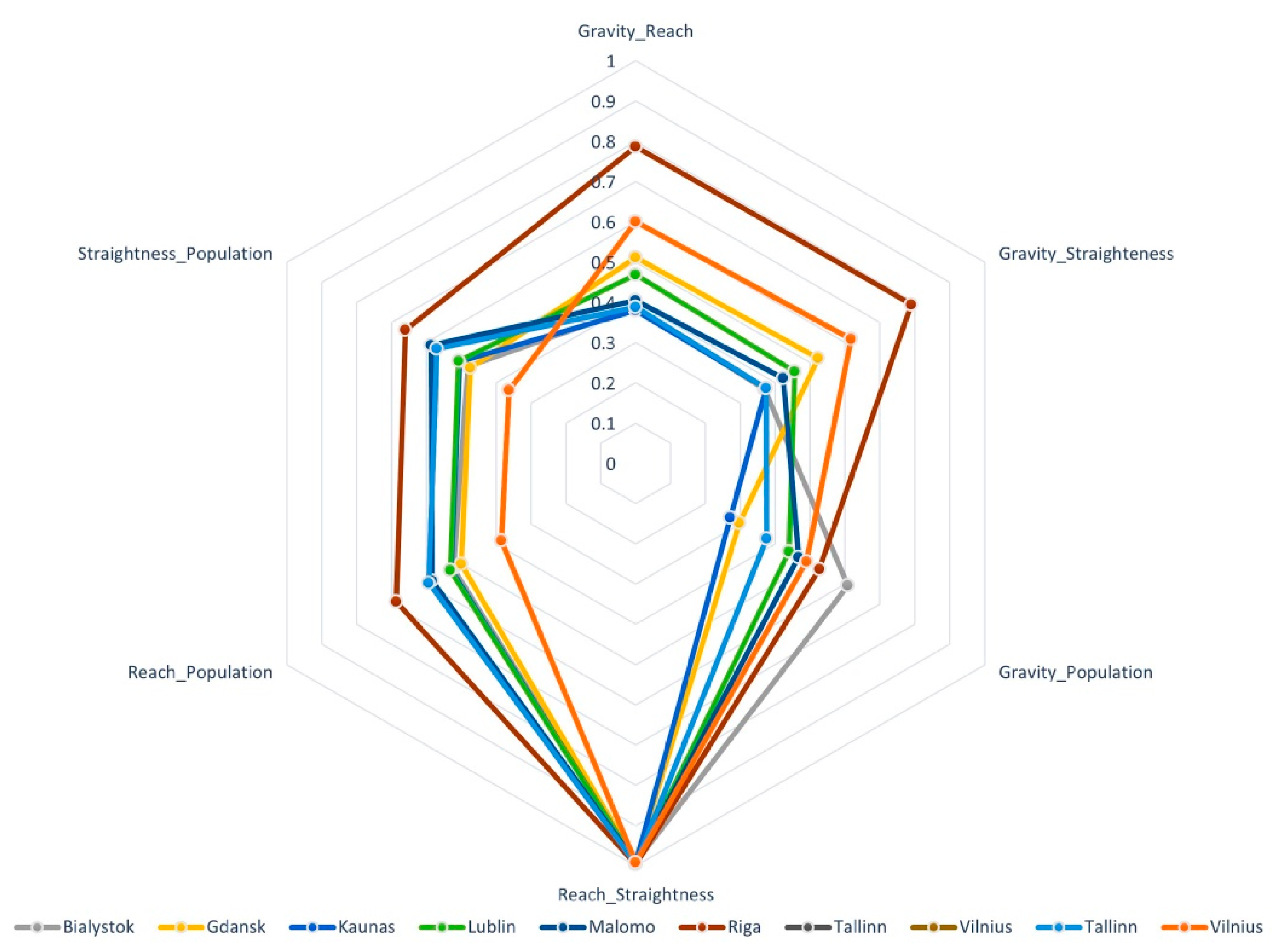
| Gr-Re | Gr-St | Gr-PoP | Re-St | Re-PoP | St-PoP | |
|---|---|---|---|---|---|---|
| Bialystok | 0.387 | 0.369 | 0.607 | 0.991 | 0.523 | 0.481 |
| Gdansk | 0.511 | 0.522 | 0.297 | 0.99 | 0.5 | 0.475 |
| Kaunas | 0.38 | 0.373 | 0.271 | 0.993 | 0.53 | 0.505 |
| Lublin | 0.469 | 0.456 | 0.439 | 0.994 | 0.532 | 0.508 |
| Malmö | 0.405 | 0.423 | 0.466 | 0.991 | 0.584 | 0.587 |
| Riga | 0.786 | 0.789 | 0.526 | 0.996 | 0.687 | 0.661 |
| Tallinn | 0.388 | 0.373 | 0.374 | 0.995 | 0.594 | 0.57 |
| Vilnius | 0.6 | 0.617 | 0.489 | 0.992 | 0.385 | 0.363 |
Publisher’s Note: MDPI stays neutral with regard to jurisdictional claims in published maps and institutional affiliations. |
© 2022 by the authors. Licensee MDPI, Basel, Switzerland. This article is an open access article distributed under the terms and conditions of the Creative Commons Attribution (CC BY) license (https://creativecommons.org/licenses/by/4.0/).
Share and Cite
Zaleckis, K.; Chmielewski, S.; Kamičaitytė, J.; Grazuleviciute-Vileniske, I.; Lipińska, H. Walkability Compass—A Space Syntax Solution for Comparative Studies. Sustainability 2022, 14, 2033. https://doi.org/10.3390/su14042033
Zaleckis K, Chmielewski S, Kamičaitytė J, Grazuleviciute-Vileniske I, Lipińska H. Walkability Compass—A Space Syntax Solution for Comparative Studies. Sustainability. 2022; 14(4):2033. https://doi.org/10.3390/su14042033
Chicago/Turabian StyleZaleckis, Kestutis, Szymon Chmielewski, Jūratė Kamičaitytė, Indre Grazuleviciute-Vileniske, and Halina Lipińska. 2022. "Walkability Compass—A Space Syntax Solution for Comparative Studies" Sustainability 14, no. 4: 2033. https://doi.org/10.3390/su14042033
APA StyleZaleckis, K., Chmielewski, S., Kamičaitytė, J., Grazuleviciute-Vileniske, I., & Lipińska, H. (2022). Walkability Compass—A Space Syntax Solution for Comparative Studies. Sustainability, 14(4), 2033. https://doi.org/10.3390/su14042033