ABIDE: A Novel Scheme for Ultrasonic Echo Estimation by Combining CEEMD-SSWT Method with EM Algorithm

Abstract

Ultrasonic echo estimation has played an important role in industrial non-destructive testing and analysis. The ability to estimate parameters in the ultrasonic echo model is crucial to ensure the effectiveness of practical ultrasonic testing applications. In this paper, a scheme called ABIDE for identifying both multiple noises in the echo signal and the distribution of the denoised signal is proposed for ultrasonic echo signal parameter estimation. ABIDE integrates complementary ensemble empirical mode decomposition and the synchrosqueezed wavelet transform (CEEMD-SSWT) as well as the expectation maximization (EM) algorithm. The echo signal is split into a series of IMF components and a residual with the help of CEEMD, and then these IMFs are classified into the noise-dominant part and signal-dominant part by analyzing the correlation of each IMF and the echo signal using grey relational analysis. Considering the effect of noise in the signal-dominant part, SSWT is adopted to remove the noise in the signal-dominant part. Lastly, the signal output by the SSWT algorithm is used for reconstructing a denoised signal combined with the residual from CEEMD. Considering the distribution characteristic of the denoised signal, the EM algorithm is used to estimate parameters in the ultrasonic echo model. The relative performance of the proposed scheme was evaluated on synthetic data and real-world data and then compared with the state-of-the-art methods. Simulation results on synthetic data show that ABIDE outperforms the state-of-the-art methods in parameter estimation. Physical results on real-world data show that the proposed scheme has a greater PCC value in estimating echo model parameters. This paper also shows that ABIDE requires less convergence time than competitive methods.

1. Introduction

Ultrasonic waves can propagate through a wide range of materials. It is convenient to choose a suitable ultrasonic transducer according to the test task to generate ultrasonic signals with desired frequencies [1,2,3]. Ultrasonic waves are often used on metals, metalloids, or other conforming materials for non-destructive testing. Due to the advantages of high automation and sensitivity and harmlessness to samples and to nearby operators [4,5], ultrasonic waves are prevalent in the domains of industry [6,7,8], material engineering [9], food engineering [10], and medical biotechnology [11] for non-destructive testing. In order to accurately detect whether there are defects or inhomogeneities in a specimen, or to accurately provide information on the size, location, nature, and quantity of the defects, a plethora of research has focused on ultrasonic signal analysis in recent years [12]. The parameter estimation of ultrasonic echoes plays an important role in ultrasonic signal analysis. As an ultrasonic echo signal is a signal expressed by a non-linear numerical model with many parameters [13,14], accurate and rapid estimation of ultrasonic echo parameters is very important for ultrasonic signal analysis.

Up to now, various methods have been proposed to estimate the parameters of ultrasonic echo signals. These methods can generally be grouped into three categories, namely, optimization methods based on the one-dimensional piezoelectric transducer model, the ultrasonic echo signal spectrum analysis model, and the ultrasonic echo parameter model. The one-dimensional piezoelectric transducer model uses one-dimensional equivalent circuit models to present the voltage-to-voltage two-way impulse response of piezoelectric transducers [15]. After considering the factors that affect the ultrasonic signal such as the diffraction and scattering of waves during the test process, the transfer function of the corresponding electrical system is deduced. Then, the parameters of the echo signal are obtained from the electrical system. Although this type of method can achieve immediate results, many factors need to be considered in the process of building a complete electrical system, such as material attenuation and dispersion transfer functions. Additionally, since the attenuation of the material is related to the material itself and the frequency of ultrasonic waves (approximate power law relationship), it is difficult to accurately estimate electrical system models. In the ultrasonic echo signal spectrum analysis model, the ultrasonic echo signal is transformed by a signal transformation (discrete Fourier transform or Gabor transform), then the corresponding echo signal spectrum is obtained, and, finally, the parameters of the echo signal are calculated by the signal spectrum [16,17]. As ultrasonic echo signals usually contain noise, this method has high uncertainty, which leads to large errors in the results. The ultrasonic echo parameter model based on optimization methods mainly focuses on the selection of optimization methods, such as the least squares estimate (LSE), artificial bee colony (ABC), ant colony optimization (ACO), and particle swarm optimization (PSO). Thus far, numerous optimization algorithms or their variants have been used for parameter estimation of ultrasonic echo signals [18,19,20]. The main difference lies in the optimization space or the efficiency. In addition, to improve the precision of the results in complex real-world issues, some scholars hold the view that increasing the signal-to-noise ratio (SNR) is of great significance; consequently, numerous works have decreased the weights of noise in raw signals [21,22,23]. Their main ideas are to improve the SNR first, and then the denoised signal is imported into the model of parameter estimation as the input. Although multiple solutions combine the denoising and optimization algorithm selection, to the best of our knowledge, both the lack of analysis on the decomposed signal selection strategy and the distribution of denoised signals still increase the overhead and hinder the precision in parameter estimation of ultrasonic signals.

In the optimization algorithm used in the parameter estimation model, noise reduction is still a necessary part. Currently, the most widely used methods in noise reduction are mostly based on the idea of the Fourier transform, moving average, and wavelet transform for effectively filtering out the noise present in the ultrasonic echo signal [24]. Since the Fourier transform is a global transformation and the sine basis function defined is a whole transformation, this means the Fourier transform is only applicable to stable frequency signals and incapable of representing local details about the signal [25]. Analysis is constrained. As to the moving average method, it loses some data points in the process of denoising, although these data points may be key data points [26]. For non-linear and non-stationary signals such as ultrasonic echo signals, the wavelet transform addresses the limitation that the Fourier transform cannot analyze the details of the signal and is applicable to nonstable frequency signals [27]. However, the drawback of wavelet transformation when applied to denoising is the poor generalization and the difficulty in selecting the basis function; thus, the selection of the basis function in the wavelet transform is application specific. Compared with the wavelet transformation, empirical mode decomposition (EMD) takes the advantages of wavelet transformation and tackles the difficulty in selecting the basis function [28]. The significant drawback of the EMD is mode mixing [29,30], which means that it cannot differentiate the intermittent signals overlapped with the raw signal. Thus, ensemble empirical mode decomposition (EEMD) has been proposed to solve this problem [31]. It utilizes the feature of the homogeneous distribution of white noise and then adds the noise to the raw signal. In this way, signals with different time scales can be automatically separated into their corresponding reference scales. Given that the method of EEMD only takes the distribution of white noise into account, complementary ensemble empirical mode decomposition (CEEMD) has been proposed to further reduce the effects of noise added with zero value of the average amplitude. The denoising method based on the CEEMD method usually judges the correlation between the inherent modal function (IMF) component and original signal by calculating their correlation coefficient, discards the components with low correlation coefficients (noise components), and keeps the components with high correlation coefficients (signal components) [32]. By combining the CEEMD and correlation coefficient methods to reduce the noise of non-stationary signals, the denoising effect is found to be better than that of the EEMD method [33]. However, simply discarding the noise components will lead to the loss of details in the reconstructed signal, especially for signals with a low SNR.

In this paper, we propose a novel scheme named ABIDE, which combines CEEMD and the synchrosqueezed wavelet transform (SSWT), as well as the expectation maximization (EM) algorithm, for ultrasonic echo signal parameter estimation. ABIDE is aware of both multiple noises in the echo signal and the distribution of the denoised signal. In particular, as for the noise-aware characteristic, ABIDE is based on CEEMD and SSWT (CEEMD-SSWT for short). In this process, firstly, the CEEMD method is used to decompose the original signal into multiple IMF components and a residual. By calculating the grey relational grades between each IMF and the original signal using grey relational analysis, the cut-off point indicating the separation of the signal-dominant part and the noise-dominant part is obtained. Considering the effect of noise in the signal-dominant part, SSWT is adopted to remove the noise in the signal-dominant part. Lastly, the signal output by the SSWT algorithm is used for reconstructing a denoised signal combined with the residual signal from CEEMD. Considering that the distribution of the denoised signal conforms to the Gaussian distribution, and that the EM algorithm is good at dealing with data with such a distribution, we input the denoised signal output via CEEMD-SSWT to the EM optimization algorithm for estimating the parameters of the ultrasonic echo.

We evaluated the effectiveness of ABIDE on synthetic data in a simulation experiment and real-world data in the physical experiment. The simulation results clearly show that ABIDE outperforms the state-of-the-art methods in parameter estimation, and that the mean absolute error of the estimated ultrasonic echo model on the input signal with an SNR of 20 dB is as small as 0.495%. The experiment results on real-world data show that the proposed scheme has greater precision, with the PCC value reaching up to 0.9903, compared to competitive methods in estimating echo model parameters. We also illustrate that ABIDE requires less convergence time than competitive methods.

The remainder of this paper is organized as follows: Section 2 presents the ultrasonic echo model for parameter estimation. Section 3 overviews the proposed ABIDE and details the components. Section 4 introduces the simulation and physical experimental setup. Section 5 describes the outcomes of the ABIDE assessment and discussion. The conclusion is presented in the final section.

2. Modeling of Ultrasonic Echo Signal

In industrial non-destructive testing applications, piezoelectric transducers are some of the most commonly used ultrasonic transducers. The shape of the ultrasonic echo is determined by the characteristics of the ultrasonic transducer and the size of defects in the sample. An ultrasonic transducer sends pulses and receives reflected echoes from discontinuities in the test sample. The time series of the ideal ultrasonic echo signal is linearly stationary and smooth, and Gaussian stochastic. The Gaussian envelope oscillation is widely used to model the ultrasonic echo function, and the Gaussian echo model (GEM) function using the time–frequency is mathematically described by the following expression:

$$s\left(\theta ,t\right)=A·e^{-\alpha {\left(t-\tau \right)}^2}·\cos \left[2\pi f_c\left(t-\tau \right)+\phi \right]$$

(1)

where $s\left(·\right)$ is the GEM signal, $\theta$ is a parameter vector, where each parameter vector contains five different variables $\theta =\left[A, \alpha , \tau , f_c, \phi \right]$, $A$ is the amplitude of the echo with the unit $\mathrm{V}$, $\alpha$ is the temporal bandwidth factor with the unit ${\left(\mathrm{MHz}\right)}^2$, $\tau$ is the arrival time with the unit $\mathsf{\mu }\mathrm{s}$, $f_c$ is the center frequency of the transducer with the unit $\mathrm{MHz}$, and $\phi$ represents the phase of the signal with the unit $\mathrm{rad}$ [34]. The details of the parameter vector $\theta$ are shown in

Table 1. Notations used for modeling of ultrasonic echo.

Symbol	Parameter	Units	Description
$A$	Amplitude	$\mathrm{V}$	According to the impedance of the transducer.
$\alpha$	Bandwidth factor	${\left(\mathrm{MHz}\right)}^2$	Establishes the bandwidth of the echo.
$\tau$	Arrival time	$\mathsf{\mu }\mathrm{s}$	Dependent on the location of the transducer.
$f_c$	Center frequency	$\mathrm{MHz}$	Related to the frequency characteristics of the transducer.
$\phi$	Phase	$\mathrm{rad}$	Reflects the orientation of the echo received.

.

In practical ultrasonic testing applications, ultrasonic echoes are commonly corrupted by additive noise, so the GEM can be rewritten as follows:

$$x\left(\theta ,t\right)=s\left(\theta ,t\right)+w\left(t\right)$$

(2)

where $w\left(t\right)$ is the additive white Gaussian noise (WGN) with variance ${\sigma }^2$ and mean zero, and $x\left(·\right)$ denotes the GEM signal corrupted by noise.

3. Methodology

3.1. Review of the CEEMD Method

The CEEMD method is an improvement and development of the EMD method [32]. The EMD method decomposes the non-stationary signal into a series of IMF components and a residual signal as follows:

$$x\left(n\right)=\sum _{i=1}^k{c}_i\left(n\right)+r_k\left(n\right)$$

(3)

where $x\left(n\right)\left(n=1,2,\dots ,N\right)$ is the original input signal, $k$ is the number of the IMF components, $c_i\left(n\right)\left(i=1,2,\dots ,k\right)$ is the IMF component where each IMF covers a certain frequency band, and $r_k\left(n\right)$ is the residual signal.

Although the EMD method is suitable for processing non-linear and non-stationary signals, the problem of mode mixing is accompanied by signal decomposition, which can easily affect the effectiveness of signal denoising [29]. In the CEEMD method, in each iteration of signal decomposition, white noise is added to the original signal in both positive and negative directions; thus, new time series signals are obtained. The EMD method is applied to the new time series signal, and the average value of all obtained IMF components by the EMD method will be the result of decomposing the new time series signal by the CEEMD method. Compared to EMD, the CEEMD method has the advantages of eliminating the problem of mode mixing and the residual noise in the original signal. The procedure of the CEEMD method for the original input signal $x\left(t\right)$ is summarized as follows:

Step 1. The positive $x_p\left(n\right)$ and negative signals $x_n\left(n\right)$ are represented by the addition of positive and negative white Gaussian noise of the same amplitude, $e_n\left(n\right)$ and $x\left(n\right)$. Mathematically, this can be expressed as Equation (4).

$$\{\begin{array}{c}{x}_p\left(n\right)=x\left(n\right)+e_n\left(n\right)\\ x_n\left(n\right)=x\left(n\right)-e_n\left(n\right)\end{array}$$

(4)

Step 2. In the process of CEEMD, the EMD method processes the positive and negative signals to obtain the sequence of the IMF components.

Step 3. Perform step 1 and step 2 for a number of times. The IMF components of the positive and negative signals are calculated as follows:

$$\{\begin{array}{c}{x}_p\left(n\right)={\displaystyle \sum _{i=1}^k}{c}_{pi}\left(n\right)+r_{pk}\left(n\right)\\ x_n\left(n\right)={\displaystyle \sum _{i=1}^k}{c}_{ni}\left(n\right)+r_{nk}\left(n\right)\end{array}$$

(5)

Step 4. According Equations (3) and (5), the decomposition outcome of the CEEMD method can be summarized as follows:

$$\{\begin{array}{c}{c}_i\left(n\right)=\frac{c_{pi}\left(n\right)+c_{ni}\left(n\right)}{2}\\ r_k\left(n\right)=\frac{r_{pk}\left(n\right)+r_{nk}\left(n\right)}{2}\end{array}$$

(6)

where $c_i\left(n\right)$ is the ultimate IMF components of the original input signal $x\left(n\right)$, and $r_k\left(n\right)$ is the residual signal. Note that the IMF components obtained by the CEEMD method are sorted in descending order according to frequency, and each IMF component reflects the contribution to the original signal.

3.2. Grey Relational Analysis

Grey relational analysis (GRA), which is an important statistical analysis method, allows for the simultaneous evaluation of more than one different objective function [35]. The idea of grey relational analysis is to judge whether the two signal sequences are closely related according to their similarity. The grey correlation grade represents the degree of similarity between the comparative sequence and the reference sequence. Additionally, the greater the grey relational grade, the greater the similarity between two signal sequences, and vice versa. GRA was used to evaluate the correlation between IMF components and the original signal in this paper. The flow chart of GRA is shown in Figure 1.

The amplitude of IMF components obtained by decomposing the original signal with the CEEMD method may vary greatly. The contribution of the IMF with a smaller amplitude to the grey correlation coefficient will be affected or even ignored. According to GRA theory, the data are processed to become dimensionless at first. The formula for dimensionless processing is described as follows:

$$y\left(n\right)=\frac{x\left(n\right)-\min x\left(n\right)}{\max x\left(n\right)-\min x\left(n\right)}$$

(7)

where $x\left(n\right)$ is the original sequence, $y\left(n\right)$ represents the normalization value of the sequence after the original data preprocessing, $y\left(n\right)\in \left[0, 1\right]$, $n\left(n=1,2,\dots ,N\right)$ is the number of data sequences, and $\min x\left(n\right)$ and $\max x\left(n\right)$ are the minimum and maximum values of $x\left(n\right)$, respectively.

After data preprocessing, the difference in the order of magnitude of the data becomes smaller. Then, the grey relational coefficient is calculated as follows:

$${\xi }_i\left(n\right)=\frac{\underset{i}{\min }\underset{n}{\min }\left|y_0\left(n\right)-y_i\left(n\right)\right|+\rho · \underset{i}{\max }\underset{n}{\max }\left|y_0\left(n\right)-y_i\left(n\right)\right|}{\left|y_0\left(n\right)-y_i\left(n\right)\right|+\rho · \underset{i}{\max }\underset{n}{\max }\left|y_0\left(n\right)-y_i\left(n\right)\right|}$$

(8)

In Equation (8), ${\xi }_i\left(n\right)$ is the grey relational coefficient. $y_0\left(n\right)$ is the reference sequence, and $y_i\left(n\right)$ is the $i^{th}\left(i=1,2,\dots ,k\right)$ comparative sequence. Now that they are all subjected to dimensionless processing according to Equation (7), $\left|y_0\left(n\right)-y_i\left(n\right)\right|$ is the deviation value between $y_0\left(n\right)$ and $y_i\left(n\right)$, and $\rho$ is the identification coefficient that represents the differentiation of data,$\rho \in \left[0, 1\right]$, and $\rho$ generally takes 0.5.

The grey relational grade can be calculated from the grey relational coefficient according to the following equation:

$${\gamma }_i=\frac{1}{N}\sum _{n=1}^N{\xi }_i\left(n\right)$$

(9)

where ${\gamma }_i$ is the overall grey relational grade for the $i^{th}\left(i=1,2,\dots ,k\right)$ GRA experiment.

3.3. SSWT Method

The continuous wavelet transform (CWT) is an effective time–frequency analysis method, which convolves a series of finite energy oscillations. CWT has the advantage of multiresolution analysis and is widely used in ultrasonic signal processing. However, CWT also has a significant disadvantage, that is, the resolution of CWT is relatively low, which easily leads to the accumulation of errors in the long-term signal processing.

As a time–frequency signal analysis algorithm, synchrosqueezing is a special reassignment method which allows the extraction of instantaneous amplitudes and frequencies, thus providing a clear, continuous wavelet representation. For some non-stationary signals, SSWT improves time and frequency resolution of CWT, which is adaptable to a wide variety of signals. The specific steps of the SSWT method are as follows.

According to CWT theory, for a signal (with noise) $x\left(t\right)$, its CWT coefficient is expressed as

$$W_x\left(a,b\right)=a^{-1/2}{\int }_{-\infty }^{\infty }x\left(t\right){\psi }^{*}\left(\frac{t-b}{a}\right)dt$$

(10)

where $W_x\left(a,b\right)$ is the corresponding wavelet coefficient of the signal $x\left(t\right)$ at a scale $a \left(a\in R_{+}\right)$ and translational (time shift) value $b \left(b\in R\right)$, $\psi \left(t\right)$ is an appropriate mother wavelet, and ${\psi }^{*}\left(t\right)$ stands for the complex conjugate of $\psi \left(t\right)$.

The estimation of the instantaneous frequency of ${\omega }_x\left(a,b\right)$ for the signal $x\left(t\right)$ is calculated as

$${\omega }_x\left(a,b\right)=-i{\left(W_x\left(a,b\right)\right)}^{-1}\frac{\partial }{\partial b}{W}_x\left(a,b\right)$$

(11)

The information from the time scale plane is transferred to the time–frequency plane, that is, the frequency variable $\omega$ and the scale variable $a$ are binned [36]. Typically, in a synchrosqueezing operation, $W_x\left(a,b\right)$ is calculated at the $k^{th}$ discrete scale value $a_k$. The synchrosqueezed transform $T_x\left({\omega }_l,b\right)$ is denoted at the central discrete angular frequency ${\omega }_l$ of the successive bins $\left[{\omega }_l-1/2·\omega , {\omega }_l+1/2·\omega ,\right]$, which can be derived as follows:

$$T_x\left({\omega }_l,b\right)={\left(\Delta \omega \right)}^{-1}\sum _{a_k}{W}_x\left(a_k,b\right)a_k^{-3/2}{\left(\Delta a\right)}_k$$

(12)

where ${\left(\Delta a\right)}_k=a_k-a_{k-1}$, $\Delta \omega ={\omega }_l-{\omega }_{l-1}$, and $a_k:\left|{\omega }_x\left(a_k,b\right)-{\omega }_l\right|\le \Delta \omega /2$.

Finally, by inverting the CWT, the original signal $x\left(t\right)$ can be obtained as follows:

$$\{\begin{array}{c}x\left(t\right)=\mathcal{R}e\left[C_{\psi }^{-1}{\displaystyle \sum _l}{T}_x\left({\omega }_l,t\right)\Delta \omega \right]\\ C_{\psi }=\frac{1}{2}{{\displaystyle \int }}_0^{\infty }{\widehat{\psi }}^{*}\left(\xi \right)\frac{d\xi }{\xi }\end{array}$$

(13)

where $\widehat{\psi }\left(\xi \right)$ is the Fourier transform of the mother wavelet $\psi \left(t\right)$, and $C_{\psi }$ is the normalization constant [37].

In order to denoise, the CWT coefficient $W_x\left(a,b\right)$ in Equation (10) is proposed via the wavelet threshold function. The wavelet threshold shrinkage denoising method including the soft threshold and hard threshold was proposed by Donoho and Johnstone [38]. For noise-containing signals, the hard threshold function method removes wavelet coefficients smaller than the threshold and retains the coefficients larger than the threshold. Instead, the wavelet coefficients larger than the threshold will be shrunk, and the coefficients smaller than the threshold will be eliminated in the soft threshold function method. Therefore, the hard threshold function method is more suitable for solving signal denoising with burst noise. However, the disadvantage of the hard threshold function method is that the result may have discontinuities at the threshold, which will generate oscillation signals and thus distortion of the noise reduction signal. The soft threshold function method is more commonly used to address the problem of diagnosing signals containing smooth noise.

Using the soft threshold function method for the original CWT coefficient, the new wavelet coefficients can be derived as

$$W_x^{\prime }\left(a,b\right)=\{\begin{array}{c}sgn\left[W_x\left(a,b\right)\right]\left(\left|W_x\left(a,b\right)\right|-Thr\right), \left|W_x\left(a,b\right)\right|>Thr\\ 0, \left|W_x\left(a,b\right)\right|\le Thr\end{array}$$

(14)

where $W_x\left(a,b\right)$ is the original CWT coefficient, $W_x^{\prime }\left(a,b\right)$ is the new CWT coefficient by the soft threshold function method, $sgn\left(·\right)$ refers to the sign function, and $Thr$ is an optimal threshold, given as

$$Thr=\sigma \sqrt{2lnN}=\frac{median\left(\left|W_x\left(a,b\right)\right|\right)}{0.6745}·\sqrt{2lnN}$$

(15)

where $\sigma$ is the standard deviation of the noise, $N$ is the length of the original signal, and $median\left(·\right)$ is the median absolute operator.

According to Equation (12), the synchrosqueezed transform ${\widehat{T}}_x\left({\omega }_l,b\right)$ of the denoised signal $\widehat{x}\left(t\right)$ in the time–frequency plane can be expressed as

$${\widehat{T}}_x\left({\omega }_l,b\right)={\left(\Delta \omega \right)}^{-1}{\displaystyle \sum }_{a_k}{W}_x^{\prime }\left(a,b\right)a_k^{-3/2}{\left(\Delta a\right)}_k$$

(16)

Under these conditions, Equation (13) can be rewritten as

$$\widehat{x}\left(t\right)=ℛe\left[C_{\psi }^{-1}{\displaystyle \sum }_l{\widehat{T}}_x\left({\omega }_l,b\right)\Delta \omega \right]$$

(17)

3.4. EM Algorithm

The EM algorithm, solving optimization problems for the observed data and the model data, is still one of the most popular algorithms for statistical recognition for models [39]. EM alternates between performing an expectation (E) step and a maximization (M) step until the parameter estimation stops updating. In the E step, the Q-function is obtained based on the likelihood function as follows:

$$Q\left(\theta ,{\theta }^{\left(t\right)}\right)={\displaystyle \sum }_{j=1}^k\left({\displaystyle \sum }_{i=1}^n\ln P\left(y_i,z_j|\theta \right)P(z_j|y_i,{\theta }^{\left(t\right)})\right)$$

(18)

where $\theta$ is the model parameter vector, ${\theta }^{\left(t\right)}$ is the parameter vector for the $t^{th}$ iteration, $y_i$ is the observed data, and $z_j$ is the latent random variable.

The E step changes depend on the data model, but the M step is independent of the model. In the M step, the maximum estimated value of the parameter vector ${\theta }^{\left(t+1\right)}$ is calculated for a new iteration which is defined as follows:

$${\theta }^{\left(t+1\right)}=arg \underset{\theta }{\max }Q\left(\theta ,{\theta }^{\left(t\right)}\right)$$

(19)

To summarize, according to the previous description of the ultrasonic echo model (see Section 2), the EM algorithm for parameter estimation of multi-Gaussian echoes in WGN can be implemented in the following steps:

Step 1. Initialize the parameter vector ${\theta }_i^{\left(0\right)}\left(i=1,2,\dots ,M\right)$ and set the iteration number $k=0$.

Step 2. The expected echoes are computed using the observed data and the current estimate of the parameter vector, that is, the parameter vector in the last iteration. Then, the $k^{th}$ iteration is performed to compute the expected echoes as follows:

$${\widehat{x}}_i^{\left(k\right)}=s\left({\theta }_i^{\left(k\right)},t\right)+\frac{1}{M}\left(x-{\displaystyle \sum }_{j=1}^{M}s\left({\theta }_j^{\left(k\right)},t\right)\right)$$

(20)

Step 3. Calculates the parameter vector ${\theta }^{\left(k+1\right)}$ as the maximum likelihood estimate for ${\theta }^{\left(k\right)}$. According to the theory of the maximum likelihood estimate, ${\theta }^{\left(k+1\right)}$ can be expressed as

$${\theta }_i^{\left(k+1\right)}=arg \underset{\theta }{\min }{\Vert {\widehat{x}}_i^{\left(k\right)}-s({\theta }_i^{\left(k\right)},t)\Vert }^2$$

(21)

Step 4. Check the convergence. As the stop criterion, the likelihood convergence tolerance ${\xi }_{LCT}\left({\xi }_{LCT}\ge 1/f^2\right)$ [40] is defined as follows:

$$\Vert {\theta }_i^{\left(k+1\right)}-{\theta }_i^{\left(k\right)}\Vert \le {\xi }_{LCT}$$

(22)

Step 5. Set the iteration number as $k\to k+1$ and go to step 2.

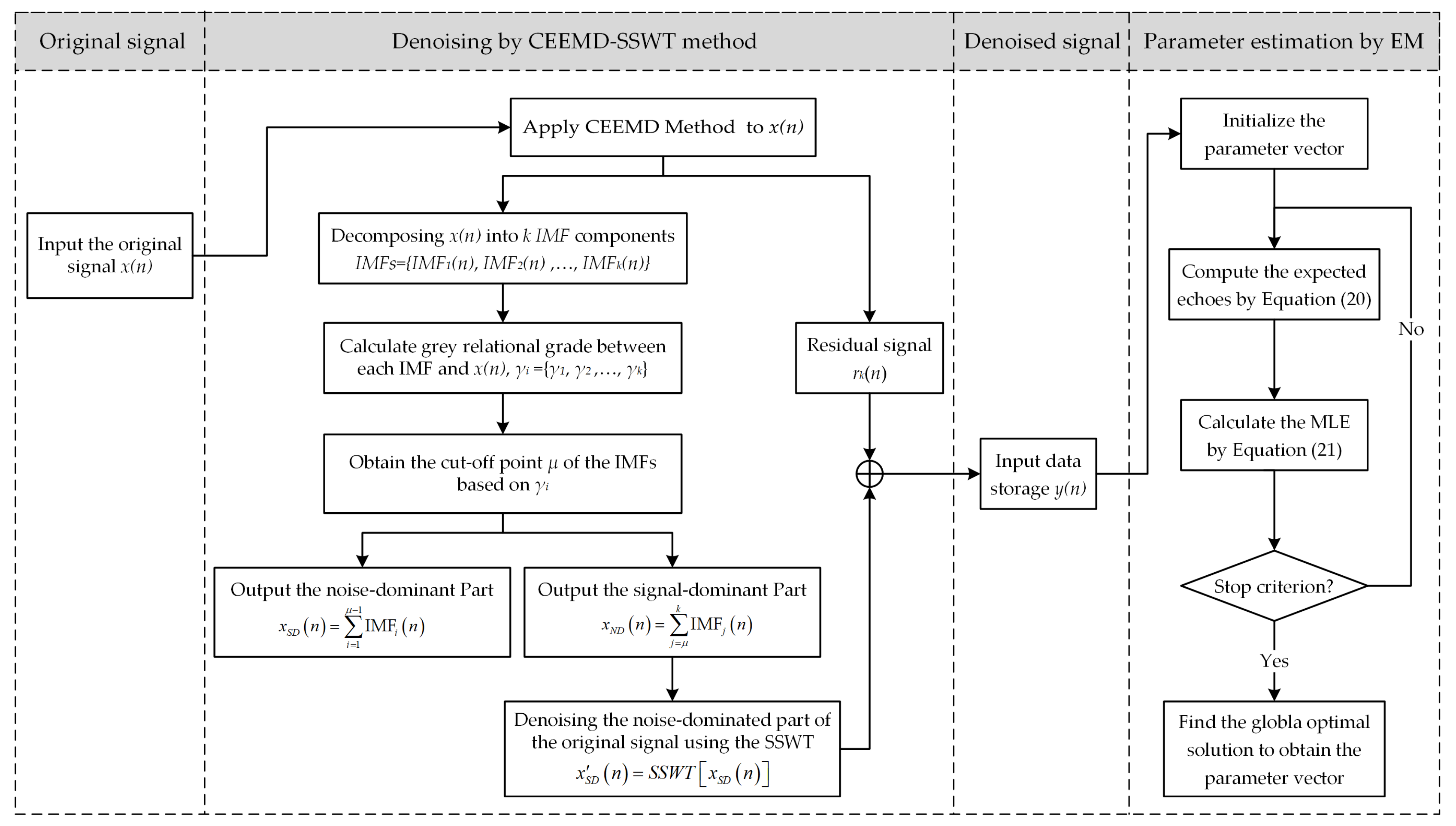
3.5. ABIDE’s Ultrasonic Echo Parameter Estimation

According to the above principles, the parameter estimation of ultrasonic echo signals in ABIDE can be derived, as shown in Figure 2, and the specific steps are as follows:

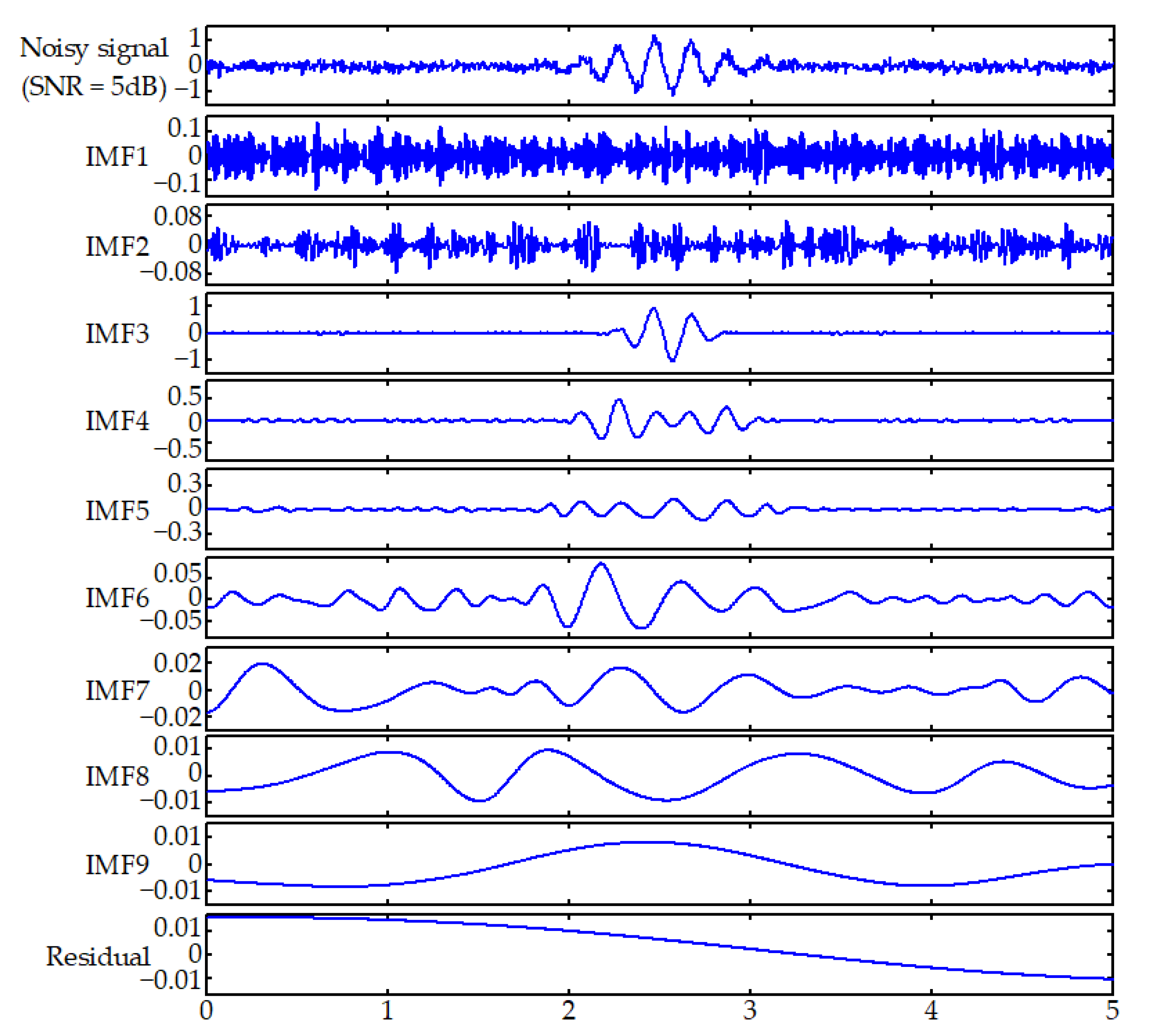
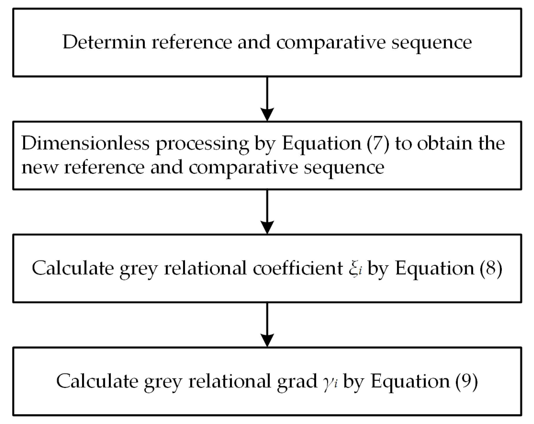
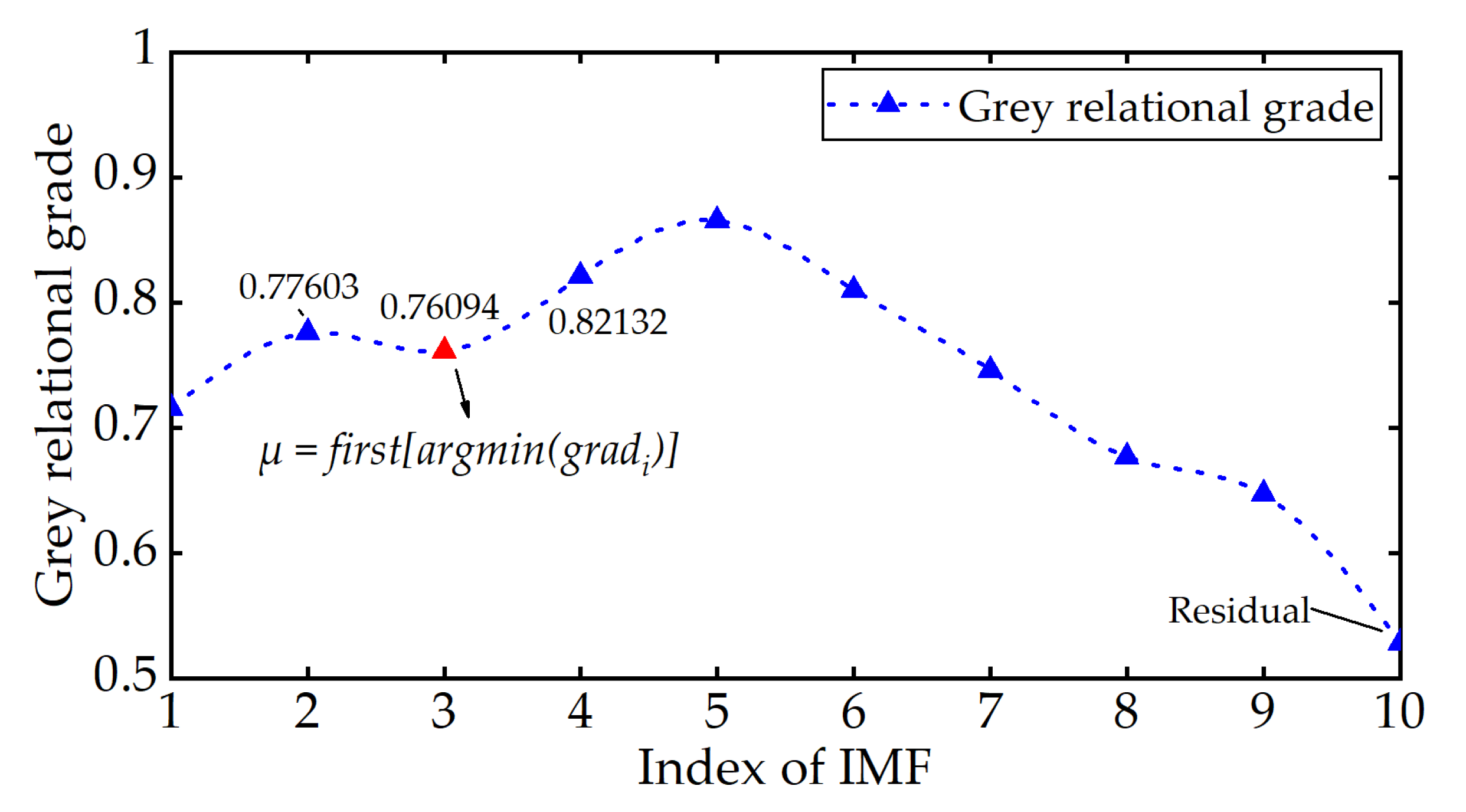
• Assuming that the original signal is $x\left(n\right)$, the CEEMD algorithm (Section 3.1) is adopted to process the original signal. $k$ IMF components $IM{F}_i\left(n\right)\left(i=1,2,\dots ,k\right)$ and a residual $r_k\left(n\right)$ are obtained. Note that the obtained IMF components are arranged in descending order of frequency. The low-order IMF includes the high-frequency part of the signal, for example, the high-frequency part of the original signal and the noise, while the high-order IMF includes the low-frequency part of the original signal, which is less affected by noise. According to grey relational theory (Section 3.2), the grey relational grade ${\gamma }_i$ between each IMF component in each order and the original signal is calculated. This process is written as

  $$\{\begin{array}{c}x\left(n\right)={\displaystyle {\displaystyle \sum }_{i=1}^k}IM{F}_i\left(n\right)+r_k\left(n\right)\\ {\gamma }_i=GRA\left(IM{F}_i\left(n\right),x\left(n\right)\right)\end{array}$$

  (23)
• Then, the cut-off point $\mu$ is determined based on the grey relational grade corresponding to the IMF component. This cut-off point is used to split the IMF decomposition into the noise-dominant part (low-order IMF components) $x_{ND}$ and the signal-dominant part (high-order IMF components) $x_{SD}$. The cut-off point criterion and signal reconstruction process are written as follows:

  $$\{\begin{array}{c}\mu =first\left[\arg \underset{1\le i\le k}{\min }\left({\gamma }_i\right)\right] \left(1\le \mu \le k\right)\\ x_{ND}\left(n\right)={\displaystyle {\displaystyle \sum }_{i=1}^{\mu -1}}IM{F}_i\left(n\right)\\ x_{SD}\left(n\right)={\displaystyle {\displaystyle \sum }_{j=\mu }^k}IM{F}_j\left(n\right)\\ x\left(n\right)=x_{ND}\left(n\right)+x_{SD}\left(n\right)+r_k\left(n\right)\end{array}$$

  (24)
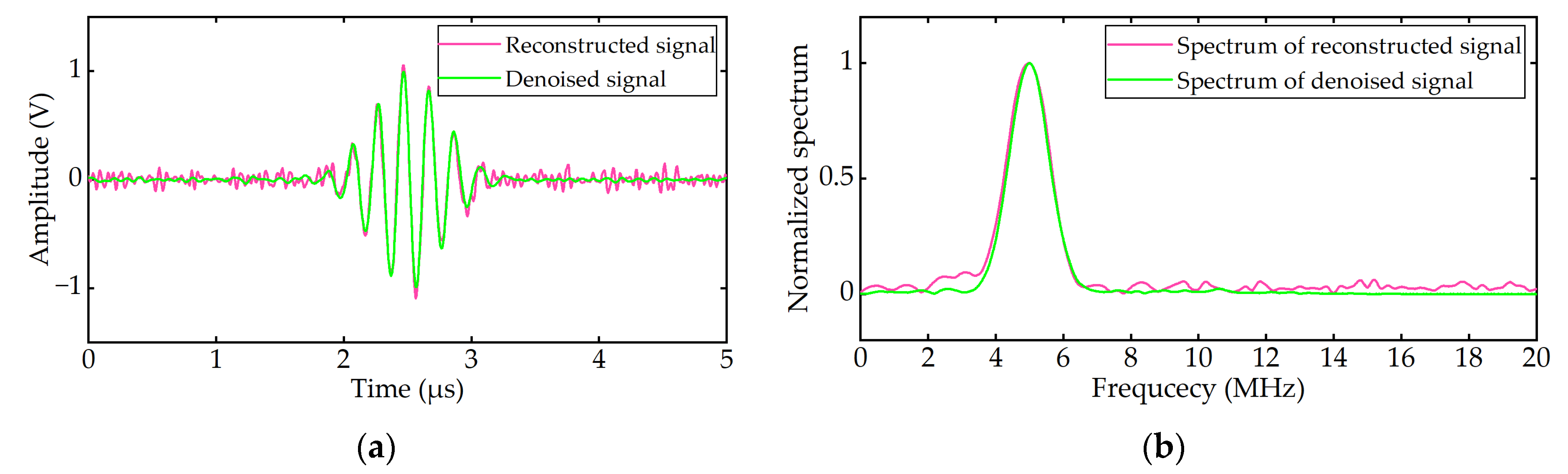
• The SSWT method (Section 3.3) is performed on the signal-dominant part $x_{SD}\left(n\right)$ to obtain the noise reduction signal $x_{SD}^{\prime }\left(n\right)$. Then, the $x_{SD}^{\prime }\left(n\right)$ and the residual signal $r_k\left(n\right)$ are reconstructed into a new input signal $y\left(n\right)$ for subsequent processing, as follows:

  $$\{\begin{array}{c}{x}_{SD}^{\prime }\left(n\right)=SSWT\left[x_{SD}\left(n\right)\right]\\ y\left(n\right)=x_{SD}^{\prime }\left(n\right)+r_k\left(n\right)\end{array}$$

  (25)
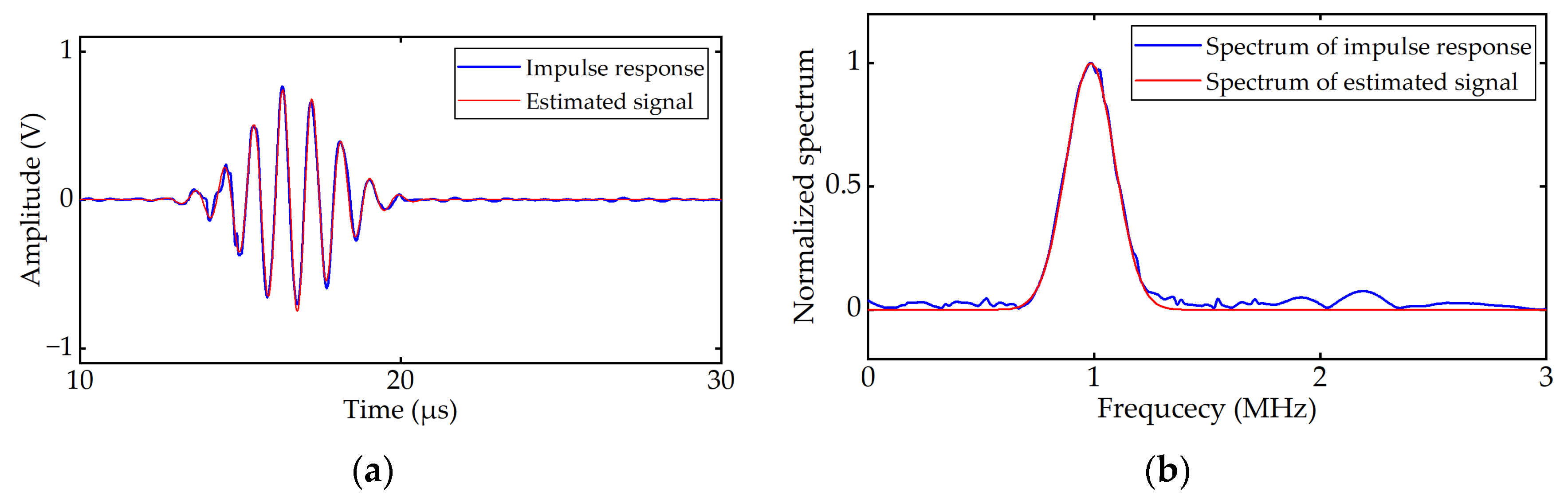
• The signal $y\left(n\right)$ obtained by the CEEMD-SSWT method is approximated by the EM algorithm (Section 3.4) which finds the global optimal solution to obtain the parameter vector $\widehat{\theta }$ of the signal $y\left(n\right)$. $\widehat{\theta }$ is defined as the model parameter vector of the original signal $x\left(n\right)$.

4. Experimental Setup and Datasets

This section is divided by subheadings. It should provide a concise and precise description of the experimental results, their interpretation, and the experimental conclusions that can be drawn.

4.1. Experimental Setup

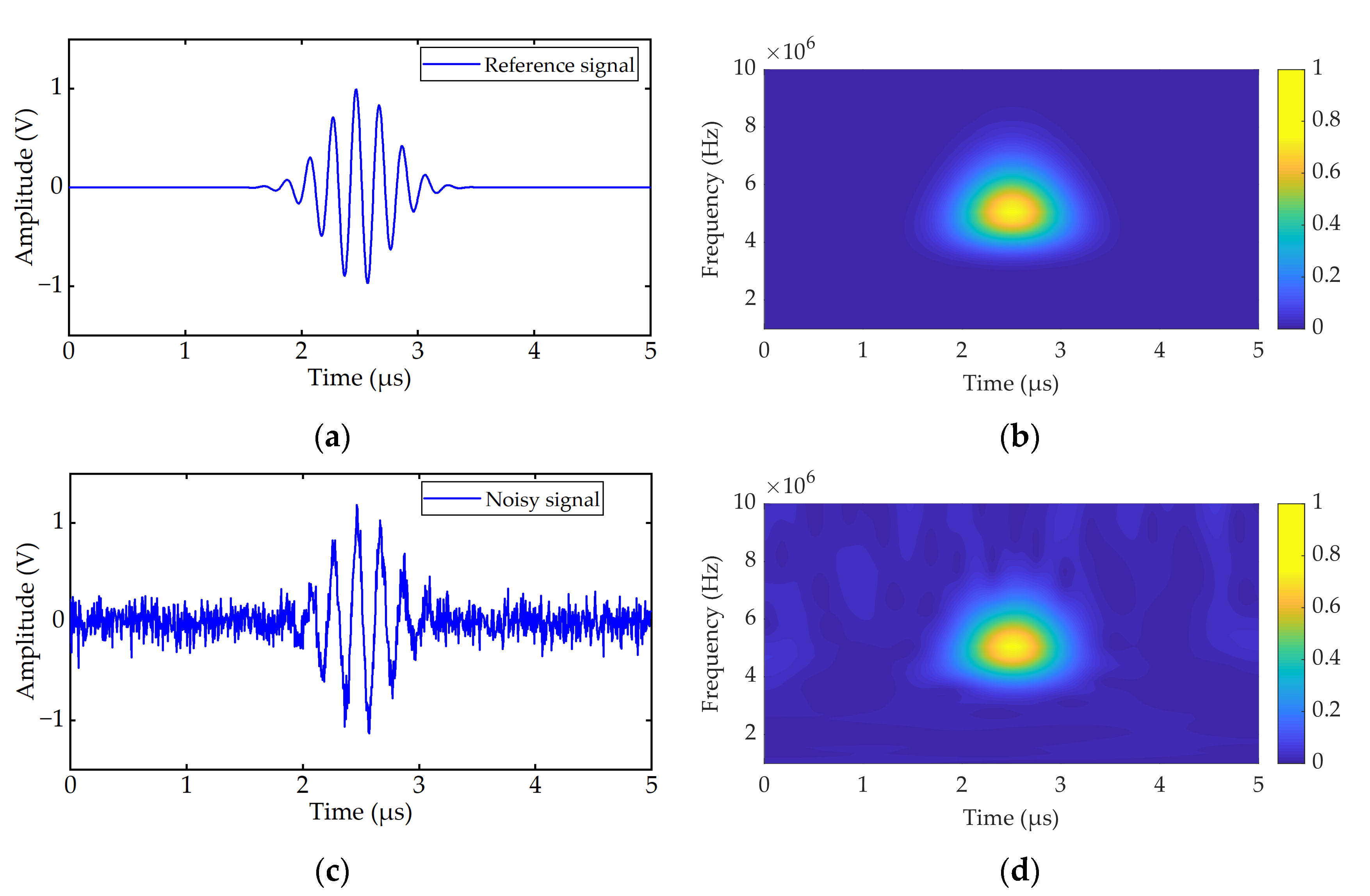
4.1.1. Simulation Experiment

The aim of the simulation experimentation was to evaluate the effect of ultrasonic model parameters estimated by ABIDE on the synthesized ultrasonic signal, and to study the denoising performance of the CEEMD-SSWT method. Since the synthesized ultrasonic signals are generated with known parameters according to the known ultrasonic signal model, the noise reduction errors and the parameter estimation errors can be determined. In order to generate datasets that approximate the ultrasonic model, the details of the experimental setup are provided. The experiment was executed on an Intel Core i5-6300U processor, internal storage 8.0 GB, Windows 10 64-bit OS. To compare the performance of the proposed scheme with the existing technology, ABIDE was also implemented in MATLAB.

The ultrasonic echo signal, utilized as the reference signal (signal generated according to the preset parameter vector) in the simulation experiment was simulated according to a modified version of Equation (1), as follows:

$$x_0\left({\theta }_0,t\left(nT\right)\right)=A_0·e^{-{\alpha }_0{\left(t\left(nT\right)-{\tau }_0\right)}^2}·\cos \left[2\pi f_0\left(t\left(nT\right)-{\tau }_0\right)+{\phi }_0\right]$$

(26)

where $t\left(nT\right)$ is the discrete samples, $T$ is the sampling interval, and $n=\left\{0,1,\dots ,N-1\right\}$ is the index of the sampling signal of length $N$.

The preset parameter vector ${\theta }_t=\left[1.0, 6.5, 2.5, 5.0, 1.0\right]$, among them, the amplitude $A_t=1.0 \mathrm{V}$, bandwidth factor ${\alpha }_t=6.5 {\left(\mathrm{MHz}\right)}^2$, arrival time ${\tau }_t=2.5 \mathsf{\mu }\mathrm{s}$, center frequency $f_t=5.0 \mathrm{MHz}$, phase ${\phi }_t=1.0 \mathrm{rad}$. This echo was sampled at a sampling frequency of 200 $\mathrm{MHz}$, that is, $T=0.005 \mathsf{\mu }\mathrm{s}$, the length of sampling data was $N=1000$, and the duration of a single simulation waveform was $5 \mathsf{\mu }\mathrm{s}$. The dataset of the reference signal was stored in vector $x_0$.

Next, noise was added according to Equation (2) considering the interferences induced by the devices or sensors in practice. A realization of a zero mean white Gaussian noise sequence with variance ${\sigma }^2$ was added to the reference signal $x_0$ to form a substitute for the original signal $x$ (the combination of the reference signal and noise). A series of simulations was performed to investigate the performance of the proposed scheme. A sequence of the original signals with an SNR ranging from 0 to 30 dB was generated.

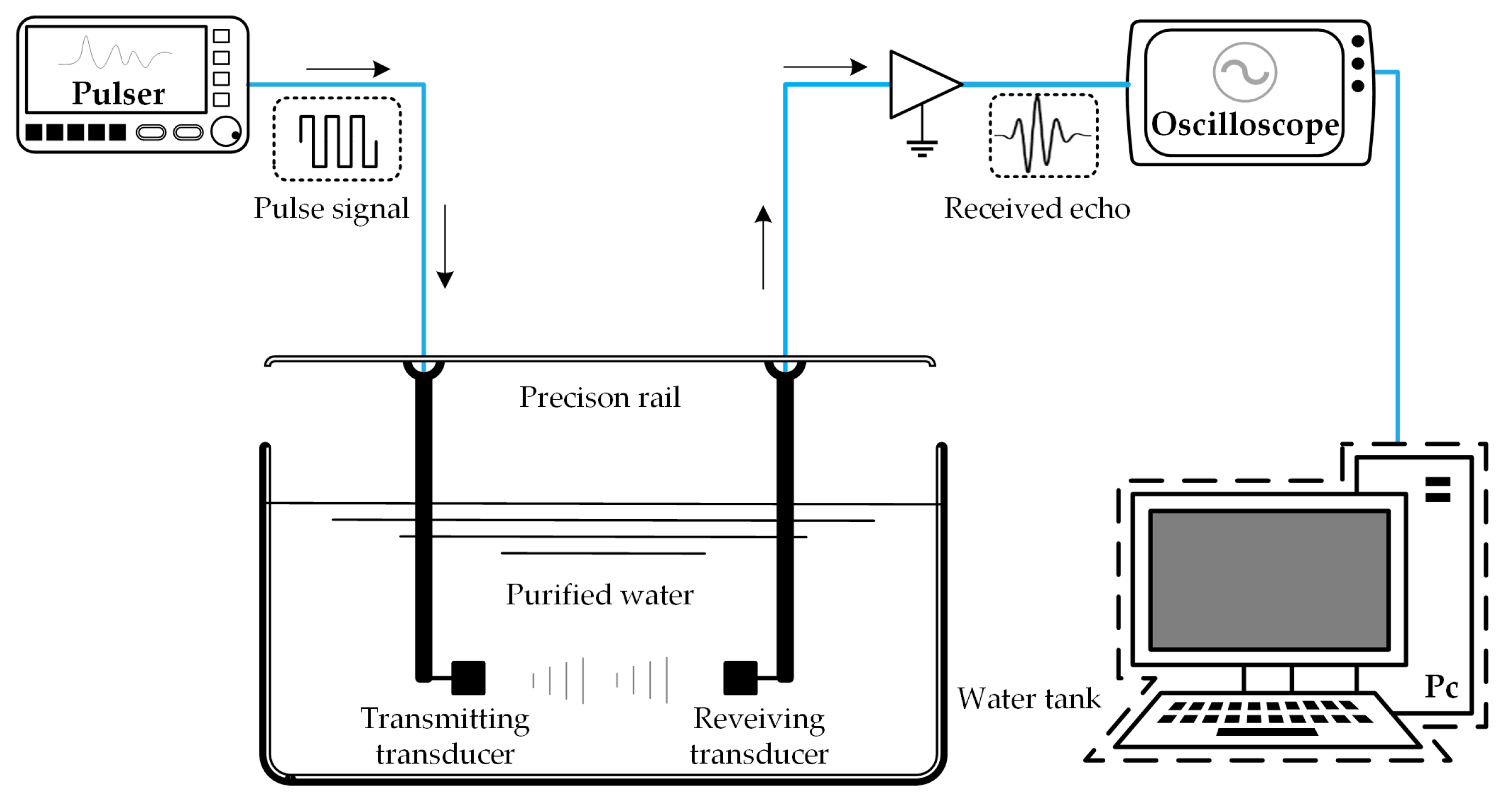
4.1.2. Physical Experiment

In this section, the performance of ABIDE is verified by an ultrasonic pulse echo system in purified water, since this experimental device is commonly used for sound velocity measurement, defect detection, and defect evaluation.

The ultrasonic echo signal was obtained by using the pulse-echo platform, and the schematic diagram is shown in Figure 3. In this schematic drawing, the platform consists of two low-cost universal ultrasonic immersion transducers, an electrically controlled displacement device for accurately determining the distance between the two transducers, a pulser, a digital oscilloscope, a water tank, and a personal computer for data acquisition. The resonant frequency of the ultrasonic transducer was 1 $\mathrm{MHz}$. The transmitting transducer and the receiving transducer were placed on the precision rail. They were immersed in purified water with a distance of 135 mm face to face.

Experimental datasets were collected by adjusting the temperature of the purified water in the water tank to 293.15 $\mathrm{K}$. The pulser was driven to send a voltage pulse signal (equal to the resonant frequency of the ultrasonic transducer) to the transmitting transducer. According to the properties of piezoelectric transducers, the pulse signal is converted into mechanical vibrations in the transmitting transducer, which, in turn, causes the generated ultrasonic waves to propagate in the aqueous medium. The propagating ultrasound waves are captured by the receiving transducer, and then the receiving transducer converts these waves into mechanical vibrations to produce an ultrasound echo signal and sends the waveform signal to the oscilloscope for further processing. The signals were recorded at a sampling frequency of 500 $\mathrm{MHz}$, and the sampling interval was $0.002 \mathsf{\mu }\mathrm{s}$.

4.2. Performance Criteria

In this section, the evaluation metrics of ABIDE are described. Specifically, the metrics for evaluating CEEMD-SSWT (denoising) and the EM algorithm (parameter estimation) in ABIDE are elaborated.

For assessing the performance of the CEEMD-SSWT denoising method, the time–frequency diagram obtained by CWT was used as the waveform of the compared signals. Moreover, the SNR, root mean square error (RMSE), and percent root mean square difference (PRD) [41] are three different common error metrics, which were used to compare the denoised signal with the original signal. The higher the SNR and the lower the RMSE and PRD, the easier the denoising effect can be attained.

Let $N$ be the length of the signal, and $x\left(n\right)$ and $y\left(n\right)$ the original and denoised signals, respectively. The SNR of the denoised signal can be expressed as

$$SNR=10\lg \frac{{{\displaystyle \sum }}_{n=1}^N{x}^2\left(n\right)}{{{\displaystyle \sum }}_{n=1}^N{\left[x\left(n\right)-y\left(n\right)\right]}^2}$$

(27)

The RMSE is defined as follows:

$$RMSE=\sqrt{\frac{1}{N}{\displaystyle \sum }_{n=1}^N{\left[x\left(n\right)-y\left(n\right)\right]}^2}$$

(28)

The PRD is calculated as follows:

$$PRD=\sqrt{\frac{{{\displaystyle \sum }}_{n=1}^N{\left[x\left(n\right)-y\left(n\right)\right]}^2}{{{\displaystyle \sum }}_{n=1}^N{x}^2\left(n\right)}}\times 100\%$$

(29)

For evaluating the performance of the EM parameter estimation method, the coefficient of determination ($R^2$) was used. $R^2$ reflects the difference between the reconstructed signal and the new input signal (denoised signal of the original signal). Moreover, the RMSE described in Equation (28) was also used to characterize the deviation of the reconstructed signal from the new input signal. Pearson’s correlation coefficient (PCC), as a complement metric, was used to evaluate the consistency between the reconstructed signal and the new input signal [42]. The optimal values of $R^2$ and PCC were close to 1. The absolute error (AE) and relative error (RE) were also employed as metrics for evaluating the error of each parameter in the ultrasonic echo model. In particular, the mean absolute error (MAE) was used to evaluate the performance of the estimation model by the proposed scheme [43]. In addition, LSE, ABC, and ACO were selected for comparison in terms of parameter estimation.

Assume that $y\left(n\right)$ is the dataset used for the model parameter estimation, that is, the denoised signal of the original signal, $\widehat{y}\left(n\right)$ is the estimated signal according to the $y\left(n\right)$, $\theta$ is the parameter vector of $y\left(n\right)$ and $\widehat{\theta }$ is the parameter vector of $\widehat{y}\left(n\right)$, and $G$ is the number of the parameter vector. Thus, the $R^2$ is determined as follows:

$$R^2=1-\frac{{{\displaystyle \sum }}_{n=1}^N{\left[y\left(n\right)-\widehat{y}\left(n\right)\right]}^2}{{{\displaystyle \sum }}_{n=1}^N{\left[y\left(n\right)-mean\left(y\right)\right]}^2}$$

(30)

The PCC is calculated as follows:

$$PCC=\frac{{{\displaystyle \sum }}_{n=1}^N\left[y\left(n\right)-mean\left(y\left(n\right)\right)\right]\left[\widehat{y}\left(n\right)-mean\left(\widehat{y}\left(n\right)\right)\right]}{\sqrt{{{\displaystyle \sum }}_{n=1}^N{\left[y\left(n\right)-mean\left(y\left(n\right)\right)\right]}^2}·\sqrt{{{\displaystyle \sum }}_{n=1}^N{\left[\widehat{y}\left(n\right)-mean\left(\widehat{y}\left(n\right)\right)\right]}^2}}$$

(31)

The AE is given as follows:

$$AE=\left|{\widehat{\theta }}_i-{\theta }_i\right|$$

(32)

The RE is fixed as follows:

$$RE=\frac{{\widehat{\theta }}_i-{\theta }_i}{{\theta }_i}\times 100\%$$

(33)

The MAE is produced using AE, as follows:

$$MAE=\frac{1}{G}{\displaystyle \sum }_{i=1}^{G}AE=\frac{1}{G}{\displaystyle \sum }_{i=1}^G\left|{\widehat{\theta }}_i-{\theta }_i\right|$$

(34)

5. Results and Discussion

5.1. Assessment on Synthetic Data

The simulated ultrasound echo signal and the noise-contaminated signal are shown in Figure 4. Concretely, the noiseless echo signal with the preset parameter vector is defined as the reference signal, as shown in Figure 4a. The time–frequency diagram of the signal was obtained with the CWT method. The magnitude plot of the reference signal is shown in Figure 4b. The noisy signal with an SNR of 5 dB and its magnitude plot are shown in Figure 4c,d, respectively.

The noisy signal was decomposed into multiple IMF components and a residual signal by the CEEMD method according to Section 3.1, and the processed results are presented in Figure 5. Obviously, IMF1 and IMF2 are both high-frequency noise signals, and all the following IMFs are a low-frequency signal. This is consistent with the characteristics of the CEEMD method. Note that not all signal decomposition results will be easily distinguished between the noise-dominant part and the signal-dominant part. For finding the cut-off point between the signal-dominant and noise-dominant parts, the grey relational grade of each IMF was calculated using the formulas in Section 3.2. These results are shown in Figure 6. According to the distribution characteristics of all obtained grey relational grades, the third value (0.76094) is the first minimum value. Therefore, the third IMF component was determined to be the cut-off point between the signal-dominant and noise-dominant parts of the noisy signal. The two IMF components (IMF1 and IMF2) in the previous part are noise signals, which are most affected by noise and are eliminated, while the last seven IMF components (IMF3–IMF9) and a residual are retained.

The reconstructed signal of the original noisy signal is obtained according to the cut-off on the IMF components. Here, IMF 3 to IMF 9 and a residual signal are accumulated to obtain the reconstructed signal. Then, noise reduction processing is performed on the IMF 3 to IMF 9 components based on SSWT to obtain the denoised IMF components. The denoised signal is reconstructed relying on the denoised IMF components and a residual. Figure 7 shows the noise reduction effect of the signals. The time–amplitude diagrams of the reconstructed and denoised signals are plotted in Figure 7a. The corresponding normalized spectrum diagrams are derived by using the Fourier transform, as shown in Figure 7b.

In order to evaluate the performance of the proposed denoising method quantitatively, SNR, RMSE, and PRD were selected as criteria in terms of noise reduction. The denoising results were calculated for different SNR noisy signals. The SNR, RMSE, and PRD for different input SNR levels were obtained, and the results are recorded in

Table 2. The consistency and SNR of the denoised signal compared with the reference signal.

Noisy Signal SNR (dB)	BayesShrink Threshold	Denoised Signal SNR (dB)	RMSE	PRD (%)
0	1.554	11.286	0.061	27.271
2.5	0.967	13.262	0.048	21.722
5	0.573	16.635	0.033	14.782
7.5	0.458	18.976	0.025	11.165
10	0.282	20.934	0.020	8.992
12.5	0.193	22.047	0.018	7.878
15	0.134	25.365	0.012	5.384
17.5	0.092	26.574	0.010	4.723
20	0.052	29.077	0.008	3.531
22.5	0.026	31.123	0.006	2.796
25	0.020	35.416	0.004	1.696
27.5	0.011	35.353	0.004	1.711
30	0.007	38.597	0.003	1.175

. It is seen that the SNR out has different improvements when the reference signal is under the influence of different degrees of noise. When the SNR of the noisy signal is 0 dB, the SNR is improved to 11.286 dB after denoising, and the RMSE is 0.061, even if the input signal is slightly poor. When the SNR of the noisy signal is 30 dB, the SNR and RMSE of the denoised signal are 38.597 dB and 0.003, respectively. Moreover, the performance of PRD is consistent with the SNR. Table 2 clearly indicates that for noisy signals with different SNR levels, a lower PRD can be obtained as the SNR changes from high to low. This means that there is a strong similarity between the denoised signal and the reference signal. The result in Table 2 presents powerful evidence that the CEEMD-SSWT denoising method performs well in boosting the SNR and tracking the consistency of the noisy signal.

The original signal was calculated using the CEEMD-SSWT method to obtain the denoised signal, which is defined as the new input signal. Then, the new input signal was used for parameter estimation of the ultrasonic echo model using the EM algorithm in Section 3.4. Typically, the parameter-seeking capability of the EM algorithm depends on the accuracy of the initial input values of the parameter. The initial value of the parameter vector ${\theta }_0=\left[A_0, {\alpha }_0, {\tau }_0, f_0, {\phi }_0\right]$ is defined as follows: The echo envelope of the new input signal is calculated using the Hilbert transform. $A_0$ is defined as the highest amplitude value of the envelope, and ${\tau }_0$ is the time corresponding to $A_0$. ${\tau }_0=2ln\left(4\right)/{\left(\mathrm{FWHM}\right)}^2$ is calculated based on the full width at half maximum (FWHM) of the envelope. The initial value for frequency $f_0$ is determined by counting the time difference $·t_0$ between two adjacent zero-crossing points of ${\tau }_0$ in the new input signal, $f_0=1/\left(2·t_0\right)$. According to the obtained parameters $\left[A_0, {\alpha }_0, {\tau }_0, f_0\right]$, the initial value of the phase ${\phi }_0$ can be obtained by solving the echo model in Equation (26). By using this rule, the initial parameter vector is calculated, and ${\theta }_0=\left[0.994, 6.462, 2.470, 4.862, 0.826\right]$.

The results of the parameter estimation for the noisy signal with 5 dB are shown in Figure 8. Concretely, the denoised signal obtained using the CEEMD-SSWT method and the estimated signal obtained using the EM algorithm are plotted in Figure 8a. The noisy signal and the estimated signal are plotted in Figure 8b. In order to evaluate the performance of the parameter estimation method, some indicators are used for a detailed discussion. The quantitative parameter estimation results of simulated signals with different SNR levels are shown in

Table 3. Results of parameter estimation for various noisy signals using the ABIDE scheme.

Simulated Signal	Echo Parameter Evaluation				Estimated Model Evaluation
	${\mathit{\theta }}_{\mathit{i}} *$	Estimated Value	AE	|RE| (%)	${\mathit{R}}^2$	RMSE	PCC	MAE (%)	ACP
SNR = 0 dB	$A$	0.958	0.042	4.233	0.961	0.065	0.959	4.496	0.922
	$\alpha$	6.568	0.068	1.045
	$\tau$	2.507	0.007	0.276
	$f$	5.017	0.017	0.345
	$\phi$	1.166	0.166	16.580
SNR = 5 dB	$A$	0.999	0.001	0.146	0.982	0.051	0.981	4.640	0.930
	$\alpha$	6.983	0.483	7.429
	$\tau$	2.504	0.004	0.146
	$f$	4.965	0.035	0.694
	$\phi$	1.148	0.148	14.786
SNR = 10 dB	$A$	1.006	0.006	0.618	0.992	0.047	0.981	1.906	0.948
	$\alpha$	6.732	0.232	3.566
	$\tau$	2.502	0.002	0.060
	$f$	4.998	0.002	0.038
	$\phi$	1.053	0.053	5.246
SNR = 15 dB	$A$	0.994	0.006	0.604	0.997	0.046	0.982	1.985	0.954
	$\alpha$	6.422	0.079	1.207
	$\tau$	2.503	0.002	0.098
	$f$	4.994	0.006	0.121
	$\phi$	1.079	0.079	7.895
SNR = 20 dB	$A$	0.988	0.012	1.175	0.999	0.047	0.983	0.495	0.960
	$\alpha$	6.478	0.022	0.339
	$\tau$	2.499	0.001	0.023
	$f$	5.000	0.001	0.006
	$\phi$	0.991	0.009	0.932

* True value of the parameter vector is ${\theta }_t=\left[1.0, 6.5, 2.5, 5.0, 1.0\right]$.

, in terms of estimated parameters, AE, RE, $R^2$, RMSE, PCC, and MAE.

From Table 3, we notice that the method has the largest estimation error for the phase, especially when the signal is contaminated with a large noise level. When the SNR is 0 dB, the relative error of the phase is 16.580%. However, with the improvement in the SNR, the accuracy of the phase estimation is increased correspondingly. When the SNR is 20 dB, the relative error of the phase is reduced to 0.932%. In addition, it is found that the EM method has advantages in estimating the arrival time and frequency, with a relative error less than 1%. In the aspect of model evaluation, using the proposed scheme, the estimated model results can be obtained under different SNR levels. The $R^2$ values are all above 0.961, and the RMSE values are below 0.065. Obviously, at 20 dB, the PCC between the estimated signal and the reference signal is up to 0.983, and the estimation error of the model is the smallest, which is 0.495%. This can be clearly seen by comparing the PCC and MAE.

The confidence interval represents the estimation range of a parameter in statistics, and the confidence level of the parameter estimation results is another reflection of the validity and robustness of a scheme. To assess the confidence level, we obtained 100 simulation signals with each SNR. These SNRs cover 0 dB, 5 dB, 10 dB, 15 dB, and 20 dB. For the 100 signals with an SNR of 0 dB, we estimated the parameter vector $\theta =\left[A, \alpha , \tau , f, \phi \right]$ using ABIDE, and the confidence interval of each parameter in the vector was obtained by calculating the average value and variance of the total estimated value. We first calculated the interval coverage probability of each parameter at the 95% confidence interval. Then, the average interval coverage probability of the confidence interval (ACP) of the parameter vector was obtained by calculating its average values. Obtaining the ACP for signals with other SNRs followed the same steps. From Table 3, we can observe that the ACP of the parameter estimation results becomes increasingly accurate with the improvement in the SNR. More specifically, when processing the signal with an SNR of 20 dB, the ACP is 0.960. Actually, when processing the signal with an SNR exceeding 10 dB, the accuracy of the parameter estimation of our scheme reached a better level.

We analyzed the residual data obtained by parameter estimation with ABIDE. Figure 9 shows the residual results of the parameter estimation for a signal with 5 dB noise. The upper left is their histogram distribution and the trend curve of a normal distribution, and the upper right is the corresponding normal probability plot of the residuals. We can see from the result that the relationship between the theoretical percentiles of the normal distribution and residual term is approximately linear. Therefore, the estimated residual term obtained by our scheme is indeed normally distributed.

In order to verify the superiority of this algorithm in ultrasonic echo parameter estimation, the proposed scheme was compared with the LSE, ABC, and ACO algorithms under the same initial conditions. The model parameter estimation results of the noisy signal with an SNR of 20 dB are shown in

Table 4. Comparison of the estimated parameters under a noisy signal with 20 dB.

Parameters and Criteria	LSE	ABC	ACO	ABIDE
$\mathrm{Amplitude} \left(\mathrm{V}\right)$	1.015	1.010	1.010	0.988
$\mathrm{Bandwidth} {\left(\mathrm{MHz}\right)}^2$	6.631	6.601	6.587	6.478
$\mathrm{Arrival} \mathrm{time} \left(\mathsf{\mu }\mathrm{s}\right)$	2.514	2.503	2.503	2.499
$\mathrm{Center} \mathrm{frequency} \left(\mathrm{MHz}\right)$	4.983	5.012	4.991	5.000
$\mathrm{Phase} \left(\mathrm{rad}\right)$	1.011	1.021	0.990	0.991
$\mathrm{Convergence} \mathrm{time} \left(\mathrm{ms}\right)$	3776	4602	6253	2811
MAE	1.104%	0.983%	0.742%	0.495%

. It can be clearly seen from the data in Table 4 that the proposed scheme in this paper has the best performance for echo model estimation, that is, the MAE (0.495%) of the model estimation is the smallest, and the fastest convergence speed ($2811 \mathrm{ms}$) can be obtained. In addition, the convergence time of the LSE algorithm is closest to that of the method proposed in this paper, but the MAE of the model estimation is the most unreliable. These results show that the proposed ABIDE has small errors and outperforms the current methods.

5.2. Assessment on Real-World Data

Using the detection system illustrated in Figure 3, ultrasonic echo signals were obtained by a pair of ultrasonic immersion transducers. In this system, a transmitting transducer is driven by the pulser to emit an excitation signal, while the other ultrasonic transducer receives the sound waves and converts them into electrical signals to be recorded. The system ensures that there is no echo overlap in the received ultrasonic echo signals. When the purified water temperature is 293.15 K, the received original echo signal is as shown in Figure 10a. Intuitively, the received echo signal has a slight high-frequency noise before 15 $\mathsf{\mu }\mathrm{s}$ and after 30 $\mathsf{\mu }\mathrm{s}$. The time–frequency diagram of the echo is shown in Figure 10b. From the diagram, in the whole time domain of the echo signal, the noise of the frequency bandwidths above 3 $\mathrm{MHz}$ is much greater than that of other frequency bandwidths.

The received echo signal was processed using the CEEMD-SSWT method to obtain the denoised echo signal. The amplitude curve and time–frequency diagram of the denoised echo signal are shown in Figure 11a,b. The denoising method effectively suppresses the high-frequency noise of the original echo signal. Different from simulated signals, the pure components of the original echo signal cannot be obtained, but the estimated SNR, RMSE, and PRD are still important for evaluating the denoising effect on the original echo signal. Assuming that a band-pass filter (0.5–1.5 $\mathrm{MHz}$) is used to calculate the reference signal, and the SNR of the denoised echo signal is 25.769 dB, the RMSE is 0.005 and the PRD is 5.033%.

The original echo signal was acquired through an analog-to-digital converter. In order to ensure that the received signal is affected by less noise, the SNR is usually improved by increasing the signal gain. The transmitting transducer used for the experiment is driven by a sinusoidal signal to work. Therefore, for the estimation of ultrasonic echo model parameters, the impulse response of the denoised echo signal was restored by applying a deconvolution method [44]. The EM algorithm was applied to the restored impulse response for parameter estimation processing, and the results obtained are shown in Figure 12. The impulse response and the estimated signal are shown in Figure 12a. A high correlation between the impulse response and the estimated signal was obtained, which can also be verified by the normalized spectrum in Figure 12b.

The results of the proposed ultrasonic echo signal parameter estimation method and the comparison results with other parameter estimation algorithms are shown in

Table 5. Comparison of the estimated parameters under a purified water temperature of 293.15 K.

Parameters and Criteria	LSE	ABC	ACO	ABIDE
$\mathrm{Amplitude} \left(\mathrm{V}\right)$	0.763	0.761	0.761	0.759
$\mathrm{Bandwidth} {\left(\mathrm{MHz}\right)}^2$	0.305	0.299	0.276	0.280
$\mathrm{Arrival} \mathrm{time} \left(\mathsf{\mu }\mathrm{s}\right)$	16.621	16.609	16.604	16.609
$\mathrm{Center} \mathrm{frequency} \left(\mathrm{MHz}\right)$	1.067	1.098	1.053	1.094
$\mathrm{Phase} \left(\mathrm{rad}\right)$	2.030	2.009	1.979	1.965
$R^2$	0.981	0.982	0.982	0.985
RMSE	0.018	0.016	0.015	0.017
PCC	0.979	0.988	0.990	0.990
$\mathrm{Convergence} \mathrm{time} \left(\mathrm{ms}\right)$	5981	6224	7320	5526

. From the values of $R^2$ and RMSE, the proposed ABIDE and the other three algorithms can successfully estimate the model parameters. Moreover, the accuracy was evaluated using the PCC between the impulse response and the estimated signal. As a result, the PCC obtained by ABIDE was 0.990, which is at the highest level. Although the accuracy of ACO is close to that of this method, the convergence time of the algorithm is longer.

Note that the signal denoising method (CEEMD-SSWT) we propose is not limited to the domain of ultrasonic signal analysis. It can be used as a signal processing tool in other fields such as lidar signals and underwater acoustic signals. As far as we know, due to the similar propagation law of ultrasonic and underwater acoustic signals in a liquid medium, it is usually necessary to rely on ultrasonic transducers to simulate underwater acoustic signals in preliminary simulation research. Therefore, the ultrasonic parameter estimation scheme we propose or its variants can also be applied to the target detection domain of underwater acoustic signals. In order to ensure the accuracy of parameter estimation results in specific applications, it is very important to research the calibration of the attribute parameters of ultrasonic transducers. In addition, we did not take multiple overlapping echoes into consideration. Further study on these aspects is necessary.

6. Conclusions

In this paper, we propose ABIDE, a multiple noise- and denoised signal distribution-aware scheme based on CEEMD, the SSWT, and the EM algorithm for estimating parameters of the ultrasonic echo model. This scheme is designed to preserve the low-frequency characteristics of the echo signal and make the accuracy of the parameter estimation less affected by the noise induced in the echo. First, a noisy echo is decomposed into a series of IMF components and a residual by the CEEMD method, and the grey relational grade is used as the similarity criterion to divide the IMF components into the signal-dominant part and the noise-dominant part. SSWT is utilized to reduce noise in the signal-dominant part. Based on the denoised signal-dominant part and a residual, the denoised signal is reconstructed and finally applied to the EM algorithm to estimate the parameters of the ultrasonic echo model. We evaluated the scheme of ABIDE in a simulation experiment and a physical experiment. We demonstrate the accuracy of ABIDE in the simulation experiment and its practicability in the physical experiment.

References

- Chen, H.; Xu, B.; Zhou, T.; Mo, Y.L. Debonding detection for rectangular CFST using surface wave measurement: Test and multi-physical fields numerical simulation. Mech. Syst. Signal Proc. 2019, 117, 238–254. [Google Scholar] [CrossRef]
- Searfass, C.T.; Pheil, C.; Sinding, K.; Tittmann, B.R.; Baba, A.; Agrawal, D.K. Bismuth titanate fabricated by spray-on deposition and microwave sintering for high-temperature ultrasonic transducers. IEEE Trans. Ultrason. Ferroelectr. Freq. Control 2015, 63, 139–146. [Google Scholar] [CrossRef]
- Zhang, Z.; Xu, J.; Yang, L.; Liu, S.; Xiao, J.; Li, X.; Wang, X.A.; Luo, H. Design and comparison of PMN-PT single crystals and PZT ceramics based medical phased array ultrasonic transducer. Sens. Actuator A-Phys 2018, 283, 273–281. [Google Scholar] [CrossRef]
- Wang, B.; Zhong, S.; Lee, T.L.; Fancey, K.S.; Mi, J. Non-destructive testing and evaluation of composite materials/structures: A state-of-the-art review. Adv. Mech. Eng. 2020, 12, 1687814020913761. [Google Scholar] [CrossRef] [Green Version]
- Rehman, S.K.U.; Ibrahim, Z.; Memon, S.A.; Jameel, M. Nondestructive test methods for concrete bridges: A review. Constr. Build. Mater. 2016, 107, 58–86. [Google Scholar] [CrossRef] [Green Version]
- Marcantonio, V.; Monarca, D.; Colantoni, A.; Cecchini, M. Ultrasonic waves for materials evaluation in fatigue, thermal and corrosion damage: A review. Mech. Syst. Signal Proc. 2019, 120, 32–42. [Google Scholar] [CrossRef]
- Pillarisetti, L.S.S.; Talreja, R. On quantifying damage severity in composite materials by an ultrasonic method. Compos. Struct. 2019, 216, 213–221. [Google Scholar] [CrossRef]
- Al-Aufi, Y.A.; Hewakandamby, B.N.; Dimitrakis, G.; Holmes, M.; Watson, N.J. Thin film thickness measurements in two phase annular flows using ultrasonic pulse echo techniques. Flow Meas. Instrum. 2019, 66, 67–78. [Google Scholar] [CrossRef]
- Wronkowicz, A.; Dragan, K.; Lis, K. Assessment of uncertainty in damage evaluation by ultrasonic testing of composite structures. Compos. Struct. 2018, 203, 71–84. [Google Scholar] [CrossRef]
- Derra, M.; Bakkali, F.; Amghar, A.; Sahsah, H. Estimation of coagulation time in cheese manufacture using an ultrasonic pulse-echo technique. J. Food Eng. 2017, 216, 65–71. [Google Scholar] [CrossRef]
- Sudarshan, V.K.; Mookiah, M.R.K.; Acharya, U.R.; Chandran, V.; Molinari, F.; Fujita, H.; Ng, K.H. Application of wavelet techniques for cancer diagnosis using ultrasound images: A review. Comput. Biol. Med. 2016, 69, 97–111. [Google Scholar] [CrossRef] [PubMed]
- Wu, B.; Huang, Y.; Krishnaswamy, S. A Bayesian approach for sparse flaw detection from noisy signals for ultrasonic NDT. NDT E Int. 2017, 85, 76–85. [Google Scholar] [CrossRef]
- Lu, Z.; Yang, C.; Qin, D.; Luo, Y.; Momayez, M. Estimating ultrasonic time-of-flight through echo signal envelope and modified Gauss Newton method. Measurement 2016, 94, 355–363. [Google Scholar] [CrossRef]
- Fierro, G.M.; Ciampa, F.; Ginzburg, D.; Onder, E.; Meo, M. Nonlinear ultrasound modelling and validation of fatigue damage. J. Sound Vibr. 2015, 343, 121–130. [Google Scholar] [CrossRef] [Green Version]
- Bybi, A.; Mouhat, O.; Garoum, M.; Drissi, H.; Grondel, S. One-dimensional equivalent circuit for ultrasonic transducer arrays. Appl. Acoust. 2019, 156, 246–257. [Google Scholar] [CrossRef]
- Lu, Z.; Ma, F.; Yang, C.; Chang, M. A novel method for Estimating Time of Flight of ultrasonic echoes through short-time Fourier transforms. Ultrasonics 2020, 103, 106104. [Google Scholar] [CrossRef] [PubMed]
- Lu, Z.; Yang, C.; Qin, D.; Luo, Y. Estimating the parameters of ultrasonic echo signal in the Gabor transform domain and its resolution analysis. Signal Process. 2016, 120, 607–619. [Google Scholar] [CrossRef]
- Zhou, J.; Zhang, X.; Zhang, G.; Chen, D. Optimization and Parameters Estimation in Ultrasonic Echo Problems Using Modified Artificial Bee Colony Algorithm. J. Bionic Eng. 2015, 12, 160–169. [Google Scholar] [CrossRef]
- Qi, A.L.; Zhang, G.M.; Dong, M.; Ma, H.W.; Harvey, D.M. An artificial bee colony optimization based matching pursuit approach for ultrasonic echo estimation. Ultrasonics 2018, 88, 1–8. [Google Scholar] [CrossRef] [Green Version]
- Yang, X.; Zhang, C.; Wang, C.; Sun, A.; Ju, B.F.; Shen, Q. Simultaneous ultrasonic parameter estimation of a multi-layered material by the PSO-based least squares algorithm using the reflection spectrum. Ultrasonics 2019, 91, 231–236. [Google Scholar] [CrossRef] [PubMed]
- Ali, M.S.S.A.; Kumar, A.; Rajagopal, P. Signal noise based transfer function approach for reliability estimation of ultrasonic inspection. Ultrasonics 2019, 96, 276–283. [Google Scholar]
- Li, J.; Liu, C.; Zeng, Z.; Chen, L. GPR signal denoising and target extraction with the CEEMD method. IEEE Geosci. Remote Sens. Lett. 2015, 12, 1615–1619. [Google Scholar]
- Zheng, H.; Dang, C.; Gu, S.; Peng, D.; Chen, K. A quantified self-adaptive filtering method: Effective IMFs selection based on CEEMD. Meas. Sci. Technol. 2018, 29, 085701. [Google Scholar] [CrossRef]
- San Emeterio, J.L.; Rodriguez-Hernandez, M.A. Wavelet Cycle Spinning Denoising of NDE Ultrasonic Signals Using a Random Selection of Shifts. J. Nondestruct. Eval. 2015, 34, 270. [Google Scholar] [CrossRef] [Green Version]
- Cooper, J.; Tran, A.N.; Wallander, S. Testing for specification bias with a flexible Fourier transform model for crop yields. Am. J. Agric. Econ. 2017, 99, 800–817. [Google Scholar] [CrossRef] [Green Version]
- Salih, S.K.; Aljunid, S.A.; Aljunid, S.M.; Maskon, O. Adaptive filtering approach for denoising electrocardiogram signal using moving average filter. J. Med. Imaging Health Inform. 2015, 5, 1065–1069. [Google Scholar] [CrossRef]
- Rhif, M.; Ben Abbes, A.; Farah, I.R.; Martínez, B.; Sang, Y. Wavelet transform application for/in non-stationary time-series analysis: A review. Appl. Sci.-Basel 2019, 9, 1345. [Google Scholar] [CrossRef] [Green Version]
- Huang, N.E.; Wu, Z. A review on Hilbert-Huang transform: Method and its applications to geophysical studies. Rev. Geophys. 2008, 46, 1–23. [Google Scholar] [CrossRef] [Green Version]
- Hu, X.; Peng, S.; Hwang, W.L. EMD revisited: A new understanding of the envelope and resolving the mode-mixing problem in AM-FM signals. IEEE Trans. Signal Process. 2011, 60, 1075–1086. [Google Scholar]
- Imaouchen, Y.; Kedadouche, M.; Alkama, R.; Thomas, M. A frequency-weighted energy operator and complementary ensemble empirical mode decomposition for bearing fault detection. Mech. Syst. Signal Proc. 2017, 82, 103–116. [Google Scholar] [CrossRef]
- Wang, T.; Zhang, M.; Yu, Q.; Zhang, H. Comparing the applications of EMD and EEMD on time–frequency analysis of seismic signal. J. Appl. Geophys. 2012, 83, 29–34. [Google Scholar] [CrossRef]
- Yeh, J.R.; Shieh, J.S.; Huang, N.E. Complementary ensemble empirical mode decomposition: A novel noise enhanced data analysis method. Adv. Data Anal. 2010, 2, 135–156. [Google Scholar] [CrossRef]
- Chen, J.; Zhou, D.; Lyu, C.; Lu, C. An integrated method based on CEEMD-SampEn and the correlation analysis algorithm for the fault diagnosis of a gearbox under different working conditions. Mech. Syst. Signal Proc. 2018, 113, 102–111. [Google Scholar] [CrossRef]
- Demirli, R.; Saniie, J. Model-based estimation of ultrasonic echoes. Part I: Analysis and algorithms. IEEE Trans. Ultrason. Ferroelectr. Freq. Control 2001, 48, 787–802. [Google Scholar] [CrossRef]
- Yazdani, M.; Kahraman, C.; Zarate, P.; Onar, S.C. A fuzzy multi attribute decision framework with integration of QFD and grey relational analysis. Expert Syst. Appl. 2019, 115, 474–485. [Google Scholar] [CrossRef] [Green Version]
- Daubechies, I.; Lu, J.; Wu, H.T. Synchrosqueezed wavelet transforms: An empirical mode decomposition-like tool. Appl. Comput. Harmon. Anal. 2011, 30, 243–261. [Google Scholar] [CrossRef] [Green Version]
- Thakur, G.; Brevdo, E.; Fučkar, N.S.; Wu, H.T. The synchrosqueezing algorithm for time-varying spectral analysis: Robustness properties and new paleoclimate applications. Signal Process. 2013, 93, 1079–1094. [Google Scholar] [CrossRef] [Green Version]
- Donoho, D.L.; Johnstone, J.M. Ideal spatial adaptation by wavelet shrinkage. Biometrika 1994, 81, 425–455. [Google Scholar] [CrossRef]
- Panić, B.; Klemenc, J.; Nagode, M. Improved initialization of the EM algorithm for mixture model parameter estimation. Mathematics 2020, 8, 373. [Google Scholar] [CrossRef] [Green Version]
- Grimes, M.; Bouhadjera, A.; Haddad, S.; Benkedidah, T. In vitro estimation of fast and slow wave parameters of thin trabecular bone using space-alternating generalized expectation–maximization algorithm. Ultrasonics 2012, 52, 614–621. [Google Scholar] [CrossRef]
- Lee, S.; Kim, J.; Lee, M. A real-time ECG data compression and transmission algorithm for an e-health device. IEEE Trans. Biomed. Eng. 2011, 58, 2448–2455. [Google Scholar] [PubMed]
- Zhou, H.; Deng, Z.; Xia, Y.; Fu, M. A new sampling method in particle filter based on Pearson correlation coefficient. Neurocomputing 2016, 216, 208–215. [Google Scholar] [CrossRef]
- Willmott, C.J.; Matsuura, K. Advantages of the mean absolute error (MAE) over the root mean square error (RMSE) in assessing average model performance. Clim. Res. 2005, 30, 79–82. [Google Scholar] [CrossRef]
- Olofsson, T. Deconvolution and model-based restoration of clipped ultrasonic signals. IEEE Trans. Instrum. Meas 2005, 54, 1235–1240. [Google Scholar] [CrossRef]