Measuring Sustainable Intensification Using Satellite Remote Sensing Data

Abstract

Farm-level sustainable intensification metrics are needed to evaluate farm performance and support policy-making processes aimed at enhancing sustainable production. Farm-level sustainable intensification metrics require environmental impacts associated with agricultural production to be accounted for. However, it is common that such indicators are not available. We show how satellite-based remote sensing information can be used in combination with farm efficiency analysis to obtain a sustainable intensification (SI) indicator, which can serve as a sustainability benchmarking tool for farmers and policy makers. We obtained an SI indicator for 114 maize farms in Yangxin County, located in the Shandong Province in China, by combining information on maize output and inputs with satellite information on the leaf area index (from which a nitrogen environmental damage indicator is derived) into a farm technical efficiency analysis using a stochastic frontier approach. We compare farm-level efficiency scores between models that incorporate environmental damage indicators based on satellite-based remote sensing information and models that do not account for environmental impact. The results demonstrate that (a) satellite-based information can be used to account for environmental impacts associated with agriculture production and (b) how the environmental impact metrics derived from satellite-based information combined with farm efficiency analysis can be used to obtain a farm-level sustainable intensification indicator. The approach can be used to obtain tools for farmers and policy makers aiming at improving SI.

1. Introduction

Over the last decades, China’s agriculture has been transforming from traditional to modern practices leading to a significant increase in the use of agricultural inputs such as fertiliser and pesticide, e.g., synthetic N fertiliser application increased from 7.07 to 26.21 million tons (a 271% increase) between 1997 and 2005 [1]. This has led to a problem of overuse of fertiliser and pesticide, which has resulted in serious pollution of water, soil and air [1,2,3,4]. This has led to calls for environmental protection [5]. In 2015, the Chinese government targeted zero growth in the use of fertilisers and pesticides by 2020 to avoid further contamination. In achieving this target, monitoring farms’ productive and environmental performance is key to identify those in need of support (e.g., advice and training). One tool that can be used to monitore is the use of remote sensing for earth observation (e.g., monitoring crop N status [6]). We use this information in combination with information on production inputs and output to (a) obtain a measure of sustainable intensification (SI) and (b) compare it with standard efficiency analysis metrics to show how incorporating an environmental dimension matters in farm efficiency scores.

Earth observation using remote sensing (i.e., satellite-based, airborne sensors and ground-based) data information has the capacity to provide useful temporal and spatial information for agriculture production analysis (e.g., crop growth), monitoring of environmental impact and externalities associated with crop production (e.g., nitrogen (N) use) [7,8]. Remote sensing can be used to help identify sustainable management practices and farmers in need of support to achieve sustainable production [7,8,9]. For instance, satellite-based data can provide useful information on the crop status as well as on crop production externalities throughout the growing season at different scales, which can be integrated into production models to forecast yields that optimise externalities and/or obtain indicators for sustainable production, which can help farm managers and policy makers to monitor and plan actions aimed at achieving sustainable production.

Here, we focus on production externalities associated with N use, both obtaining and integrating an indicator for externalities associated with N use into a stochastic frontier analysis. Although N is essential for plant growth, excessive N application can lead to environmental degradation. We integrate available satellite-based remote sensing information on N use at the farm-level using information on farm coordinates with farm-level data obtained through a survey into a farm efficiency analysis to obtain an indicator of SI, which can serve as a benchmarking tool for farmers and policy makers aiming at improving farm environmental sustainability.

The paper is organised as follows. Section 2 provides an overview of the main approaches used to measure sustainable intensification. This section explains how production externality indicators (e.g., environmental impact indicators, including satellite derived leaf area index) can be incorporated into standard efficiency analysis to obtain sustainable intensification metrics. In Section 3, we describe the materials and methods used to conduct the analysis. Here, we describe the data used as well as the development of environmental impact and sustainability indicators, their incorporation into an efficiency model and the model estimation process. Section 4 presents the results for a standard model, which does not include the environmental output (Model 1) and a model that incorporates a satellite-derived environmental impact indicator (Model 2). Section 5 discusses the results and Section 6 presents the conclusions we can extract from the analysis.

2. Measuring Sustainable Intensification

SI is seen as a possible way to tackle the problem of having to increase food production, as a consequence of an increasing population, whilst protecting the environment [9,10]. As pointed out by [11], a precise definition of SI is not possible with SI being a concept with different interpretations and definitions that overlap between them [12]. Such differences in the interpretation and definition of SI are rooted in both the spatial heterogeneity found in the environmental context, the heterogeneity of production systems employed and the different views held by stakeholders on what SI means to them [10,12]. Hence, a wide range of approaches have been used to develop SI metrics covering a variety of aspects such as productivity, economic sustainability, environmental sustainability, social sustainability and human wellbeing [13]. One of the stems to achieve SI is through assessing farmers’ performance (i.e., using farm-scale metrics) [14]. However, many of the SI indicators/metrics developed are individual indicators that capture a single aspect within SI, which may have a limited use, especially in agricultural systems that produce multiple outputs including positive and negative externalities associated with the use of agricultural inputs (e.g., fertilisers). Some of these individual indicators are ratios of units of output per unit of environmental impact or pressure [15]. Consequently, composite indicators using weights to aggregate individual indicators have been developed to overcome the limitations of individual indicators. However, these type of composite indicators do not directly account for interactions between inputs, outputs and externalities. One way to integrate negative externalities indicators and market outputs is through incorporating production externality indicators into an efficiency and productivity analysis of non-agricultural activities using non-parametric and parametric approaches, such as data envelopment analysis (DEA) and stochastic frontier analysis (SFA) [16,17,18]. DEA approaches started to be applied to the efficiency analysis of agricultural activities [19,20] as well as stochastic frontier analysis (SFA) approaches [21]. Accounting for positive externalities in the efficiency analysis was applied later by [22]. This earlier work led to the development of sustainable production and SI metrics that incorporate environmental aspects (positive and/or negative externalities) into efficiency analysis, either using stochastic frontier analysis (SFA) or data envelopment analysis (DEA) [12,23,24,25]. The first to derive an SI indicator from efficiency analysis using DEA was [24]. However, the eco-efficiency literature and work on the development of farm-level metrics that account for both market and environmental outputs from farming (negative and positive externalities) using DEA (e.g., [15]) and SFA approaches could also be used/interpreted as indicators for SI. The authors of [12] point out how eco-efficiency and SI are actually closely related concepts.

SFA and DEA approaches that integrate agricultural production with its externalities to obtain SI metrics can be embedded within a production possibilities frontier (PPF) framework with two dimensions: agricultural production and provision of environmental goods/ecosystem services [26,27]. These approaches can calculate an index that weights as a single value the different ecosystem service (i.e., positive externalities) with agricultural production. However, as pointed out by [11,12], the trade-off between agricultural and ecosystem service provision is not known in practice due to being a combination of multiple ecosystem services, and it varies across space. In the same way, it is acknowledged that the environmental impact associated with agricultural production cannot be easily measured and in most of cases it is unknown, making the use of environmental indicators the best possible option available.

The leaf area index (LAI), which is defined as half the total area of green elements of the above-ground portion of a crop per unit horizontal ground area, can be used to derive a metric of maize N uptake. The use of LAI as an indicator for plant N uptake has been previously validated [28]. Consequently, we use LAI to provide an estimate of N concentration ($N_c)$ in maize [28], which we use as an indicator of environmental damage associated with maize production. Hence, we combine information on N’s environmental impact/damage, using a satellite-derived LAI, with farm production factors and farm output to derive a sustainability measure/sustainable intensification measure that accounts for both the use of inputs and the environmental damage associated with Nitrogen use in maize production. Remote sensing data offers an opportunity to incorporate relevant information on typically non-observed farm production externalities. We show how satellite-based remote sensing data can be used to account for externalities associated with N use in maize production and be incorporated into SFA to obtain a farm-level SI indicator.

3. Materials and Methods

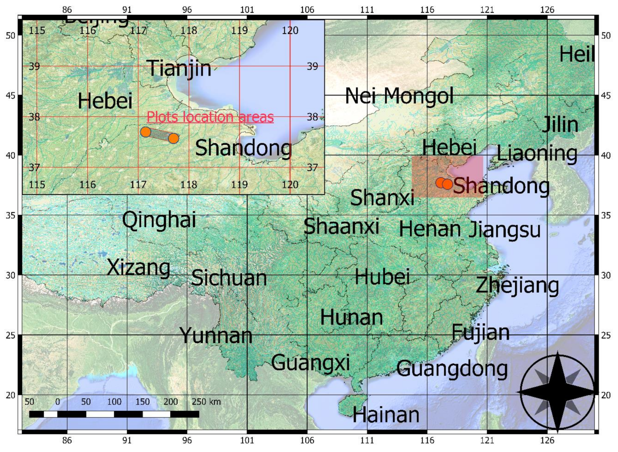
In this section, we describe the data used in the analysis including the location of the survey conducted and information collected. In addition, we explain how we derived a farm-level sustainability indicator by incorporating an environmental impact indicator associated with maize production using satellite data into efficiency analysis. Finally, we explain how the models used are estimated and their predictive capability is evaluated.

3.1. Data

We used a survey dataset of 114 maize farmers in Yangxin County located in Shandong Province in China (Figure 1) who were interviewed face-to-face between October 2018 and February 2019. Shandong province is China’s highest wheat and maize producer. The survey collected information on the quantity of maize output produced (kg); inputs used included the cultivated area (mu), seed cost (Chinese Yuan), fertiliser cost (Chinese Yuan), crop protection cost (Chinese Yuan), labour used (total number of hours) and location coordinates of the plots. Mu is a land measurement in China, where 1 mu is approximately 0.067 ha. We also collected information on the LAI from the European Commission Copernicus services (land, atmosphere and emergency management services). The LAI index was averaged for each field over the maize growing season period, which runs between June 2018 and October 2018. The growing season was determined by using information provided by farmers in the sample on planting and harvesting dates.

3.2. Environmental Impact and Sustainability Indicators

We obtained an environmental impact indicator associated with maize production using satellite data. This environmental impact indicator is used to derive a farm-level sustainability indicator that accounts for the interrelationship between crop production and the negative externalities associated with N overuse (i.e., negative impact on the environment) using an efficiency analysis framework. For this, we first derive a proxy for environmental damage due to N use (using estimated N usage at the farm-level from satellite-based remote sensing data). It is worth pointing out that we evaluated a range of possible suitable environmental indicators (EIs) available from earth observation (EO) data provided by the European Commission Copernicus services (land, atmosphere and emergency management services) that could be used for our analysis. We did not find as many indicators as initially expected that could be used as environmental indicator associated with maize production using this non-commercial satellite data source. Furthermore, we found that the spatial resolution of most of the data was not adequate for the spatial distribution of the farms studied. However, as pointed out above, we found an indicator, the mean leaf area index (LAI), to obtain an indicator of environmental impact associated with N use. Since the data contain information on the location of the farm (coordinates), we could match the farms to the LAI and calculate for each plot the average LAI during the maize growing period. We used daily LAI over the maize growing season (June 2018–October 2018), obtained from the European Commission Copernicus services, from which we calculated its average over the summer growing season for each maize plot. The LAI spatial resolution is 300 m, which is estimated by applying a neural network on instantaneous top-of-canopy reflectances from Sentinel-3 OLCI (v1.1 products), or daily top-of-aerosol input reflectances from PROBA-V (v1.0). For further detailed information on LAI data (e.g., algorithm, quality, validation and technical characteristics) used please visit Leaf Area Index|Copernicus Global Land Service. Using the farm-level LAI values we obtained a critical N concentration ($N_c$) [28,29]. Critical content of nitrogen is the minimum N concentration in shoot biomass and specific plant organs, e.g., leaves, stem and leaf area index, (i.e., aboveground dry matter, % DM) required for maximizing growth rate in the plant measured in Mg N g-1 dry biomass units. Knowing the crop $N_c$ can help to optimize yield as well as reduce environmental impact by better managing N use [30]. Following [29], we calculated the $N_c$ for maize as follows

$$N_c=3.84LA{I}^{-0.45}$$

(1)

where LAI is the average leaf area index over the maize growing season for maize. Equation (1) shows that the higher the LAI is, the lower the $N_c$ is (i.e., the nitrogen use is relatively high and the nitrogen concentration needed to maximise growth is relatively low). In order to facilitate interpretation, we changed the sign of $N_c$. In this case, relatively high (low) $N_c$ values indicate relatively high (low) risk of environmental damage.

Equation (1) establishes a theoretical framework to link the relationship between LAI and Nc for summer maize in China [29]. Hence, Equation (1) can be applied with confidence to summer maize grown in China and could potentially be applied to other parts of the world. However, confirmation requires further research. Although parameters of LAI-based curves change across different species (rice, wheat and maize) [29], it was also found that dry matter-based nitrogen concentration measures developed for summer maize in France are also applicable to Germany and eastern Canada [29].

The $N_c$ was previously used to calculate N nutrition index (NNI) used to determine the crop N nutrition status [31]. Since all farms are located in the same province (i.e., facing similar environmental conditions) the use of $N_c$ as an indicator for (risk to) environmental damage is independent of such conditions. We expect the coefficient of this indicator to be positive, indicating that the greater the value of the $N_c$(i.e., the higher the risk of environmental damage) the higher the maize output. This would capture a trade-off between higher maize output and protecting the environment.

Table 1. Data descriptive statistics.

Variable	Mean	Std. Dev.
Maize production (kg)	6298	4010
Maize area (mu)	10.9	6.1
Fertiliser cost (Yuan)	141.1	40.0
Crop Protection cost (Yuan)	20.7	12.0
Labour (hours)	186.2	90.1
Nitrogen Use Indicator (Nc)	2.9	0.3

shows the descriptive statistics of the data used in the analysis.

3.3. The Efficiency Model

We used two alternative models, one which would be the standard efficiency analysis that does not account for environmental impact associated with N use (Model 1), and a second model which incorporates the environmental impact indicator based on the nitrogen concentration (Model 2).

We used a distance function framework to account for the multi-output multi-input production process. We described the set of both output vectors, maize and negative externalities associated with nitrogen use (Model 2) in the output/production possibility set $P\left(x\right)$.

$$P\left(x\right)=\left\{y\in {ℝ}_{+}^M:”x can produce y” \right\}=\left\{y:\left(x,y\right)\in T\right\}$$

(2)

where $y$ refers to all $M$ farm outputs, maize and negative externalities associated with nitrogen use, which for Models 2 and 3 include the environmental impact and damage indicators, respectively; $x$ all $K$ inputs used, and $T$ is the production technology set. The distance function is defined in the output set as

$$D_O\left(x,y\right)=“min” \left\{\theta :y⁄\theta \in P\left(x\right)\right\}” for all “ x \in {ℝ}_{+}^K$$

(3)

We parameterised the distance function as a Cobb–Douglas function, defined over M outputs and N inputs:

$$\ln D_{0i}={\alpha }_0+{\displaystyle \sum }_{m=1}^M{\alpha }_m{y}_{mi}+{\displaystyle \sum }_{k=1}^K{\beta }_k\ln X_{ki}, i=1,\dots ,N$$

(4)

where $D_{0i}$ denotes the output-oriented distance function; $\alpha$’s and $\beta$’s are parameters to be estimated; $y_{mi}$ is the $m$ output (maize, environmental externality) of the $ith$ farm in the sample; $x_{ki}$ is the quantity of input $k$ used in the $ith$ farm in the sample. We normalised Equation (5) by maize production to transform it into an estimable regression, which leads to the following estimable function.

$$-\ln y_1={\alpha }_0+{\displaystyle \sum }_{m=1}^M{\alpha }_m\frac{y_{mi}}{y_1}+{\displaystyle \sum }_{k=1}^K{\beta }_k\ln x_{ki}-\ln D_{Oi},=1,\dots ,N$$

(5)

Using matrix notation, we can represent the model as follows:

$$y=X\beta +\epsilon -z$$

(6)

where $y$ is a $N\times 1$ vector that denotes the farms’ logged maize production; $X_i$ is a matrix of the farms’ logged production inputs and negative externality (environmental impact and damage indicators); $\epsilon$ is a normal error term and $z$ is the farms’ inefficiency term, which follows a Gamma distribution. The critical N concentration $N_c$ is normalized by the main output (maize) and all variables in the model are standardized.

3.4. Model Estimation

We used a Bayesian approach with Markov chain Monte Carlo (MCMC) sampling to estimate the conditional posterior distribution of the parameters of the frontier model ($\beta ,\sigma ,z$). Under this approach, we assumed a normal conditional distribution for the production function

$$y ~ N\left(X\beta +\epsilon -z,\sigma \right)$$

(7)

with weakly informative priors for $\beta ~ N\left(0,10\right)$; $\sigma ~ Cauchy\left(0,10\right);$ $z ~ G\left(1, \left(1/-log\left(0.85\right)\right)\right)$. We ran 4 chains with 5000 iterations each, discarding 2500 in each chain, meaning there were a total of 10,000 total draws retained. We used the Watanabe–Akaike information criterion (WAIC) and the leave-one-out-cross-validation (LOO-CV) method since these measures allow for evaluating model predictive capability, without the need to re-estimate the model on a cross-validation set. In addition, we use WAIC and LOO-CV to compare both models’ predictive performance. A lower WAIC and LOO-CV indicate a better predictive model. Analysis of the data was performed using the rstan package v2.21.2 [32,33].

4. Results

This section first presents the mean coefficients associated with inputs (Model 1) and the environmental impact (Model 2) of the MCMC sample observations for Model 1 (standard efficiency model) and Model 2 (incorporating an environmental impact indicator based on the Nc). Secondly, it presents predictive performance statistics for each model. Thirdly, we present the mean efficiency estimates across maize farms in the sample for the two models. Finally, we compare the farm efficiency rankings obtained from both models.

4.1. Coefficient Estimates Associated with Production Inputs and Outputs

Table 2. Model 1 parameter estimates.

Logged Variable	Mean Coeff.	95% Posterior	$\widehat{\mathit{R}}$
Intercept	0.25	(0.21–0.29)	1.0
Maize area	0.93	(0.86–1.00)	1.0
Fertiliser cost	0.01	(0.00–0.03)	1.0
Crop Protection cost	0.02	(0.00–0.04)	1.0
Labour	0.06	(0.02–0.11)	1.0

and

Table 3. Model 2 parameter estimates.

Logged Variable	Mean Coeff.	95% Posterior	$\widehat{\mathit{R}}$
Intercept	0.18	(0.15–0.21)	1.0
Maize area	0.72	(0.66–0.79)	1.0
Fertiliser cost	0.01	(0.00–0.02)	1.0
Crop Protection cost	0.02	(0.00–0.05)	1.0
Labour	0.03	(0.01–0.07)	1.0
Environmental impact indicator	0.45	(0.40–0.49)	1.0

show the mean coefficients as well as the 95% coverage posterior region (i.e., the fifth and ninety fifth percentiles of the parameters’ conditional posterior distributions) for the standard model, which does not include the environmental output (Model 1), and the model that incorporated the environmental impact indicator (Model 2). All inputs in both models are positive, complying with monotonicity (i.e., an increase in the use of inputs does not lead to a decrease in output). There are no relevant differences between coefficients obtained in the two models, except for the coefficient associated with area allocated to maize production. The positive coefficients of production inputs in Model 1 indicate that a 1% increase in area fertiliser, crop protection and labour yields a 0.93%, 0.01%, 0.02% and 0.06% increase in maize output. The results from Model 2 indicate that a 1% increase in area fertiliser, crop protection and labour yields a 0.72%, 0.01%, 0.02% and 0.03% increase in maize output. Model 2 also predicts that a 1% increase in environmental impact associated with N use would lead to a 0.45% increase in maize output. Hence, the positive coefficient associated with the environmental impact indicator (Nc) in Model 2 indicates that the higher the environmental risk by N use is, the higher the maize output per ha, capturing the trade-off between the damage associated with nitrogen use and maize output. In addition, we compared the between- and within-chain estimates for model parameters, which showed no indication of chains not mixing well. Table 2 and Table 3 also report on the $\widehat{R}$ ratio, which indicates all chains for each parameter estimated have converged (i.e., values of $\widehat{R}<1.1$) [31]

4.2. Predictive Model Performance

Table 4. Model predictive performance statistics.

Predictive Performance Statistic	Model	Estimate	Std. Error
elpd_waic	1	−12.71	9.01
elpd_waic	2	20.47	12.32
WAIC	1	25.42	18.02
WAIC	2	−40.93	26.64
elpd_loo	1	−26.50	12.60
elpd_loo	2	8.10	15.6
LOO-CV	1	52.90	25.10
LOO-CV	2	−16.20	31.20

shows results for statistics measuring model predictive accuracy. The results in Table 4 suggest that Model 2 is preferred to Model 1 using both predictive performance statistics. To determine whether the difference is significant, we calculated a z-score and compared it with a standard normal distribution using the expected log pointwise predictive density (elpd) difference between both models. For the WAIC’s elpd between models, the $Pr\left(z\ge \frac{-33.2}{8.9}\right)={9.56}^{-5}$ indicates that Model 2 outperforms Model 1. Likewise, for the LOO-CV’s expected log pointwise predictive difference between models, the $Pr\left(z\ge \frac{34.6}{11.1}\right)={9.13}^{-4}$ also indicates that Model 2 outperforms Model 1.

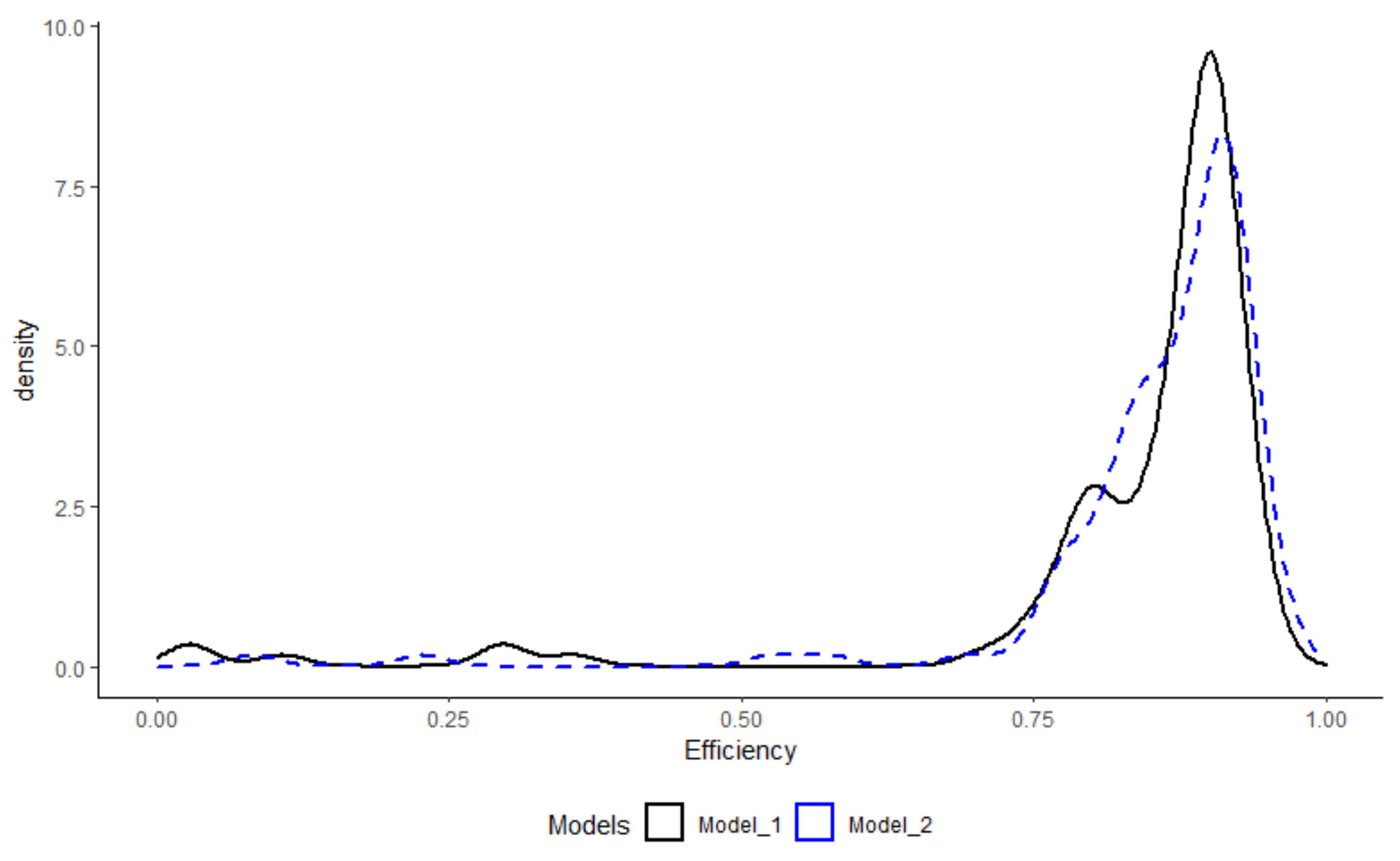
4.3. Farm Efficiency Estimates

Figure 2 shows the conditional posterior distributions for mean efficiency across maize farms in the sample for the two models. The efficiency scores of the sample range between 0.03 and 0.95 under Model 1 and 0.08 and 0.96 under Model 2, with median 0.89 under both models. The average efficiency under Model 1 is 0.84, whereas the average efficiency under Model 2 is 0.86. By examining the probability of efficiency scores obtained using Model 2 which were greater than when using Model 1, we find that 64% of efficiency estimates are greater under Model 2 than under Model 1. These results indicate the estimated farm plot efficiency levels slightly increase when accounting for environmental impacts in the stochastic frontier. However, the absolute difference in the mean efficiency scores is relatively small, making both distributions relatively similar (Figure 2). In any case, despite mean efficiency distributions being relatively similar, there may be differences in farms’ rankings between the different models used, which may have important implications for policy making [12,22]. This is relevant for cases where policy making aims at providing support to farmers who may need to improve their sustainability. Using a standard approach to identify farmers who can improve their sustainability performance (i.e., environmental indicators are not incorporated in the efficiency analysis) may lead to the provision of support to the wrong farmers.

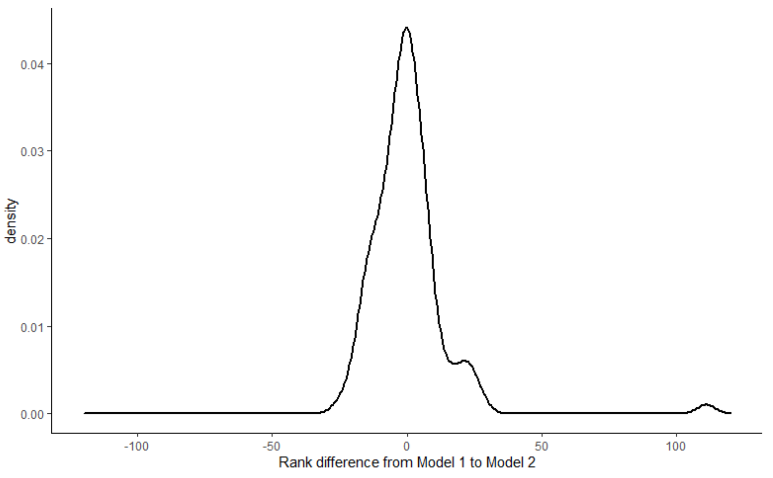
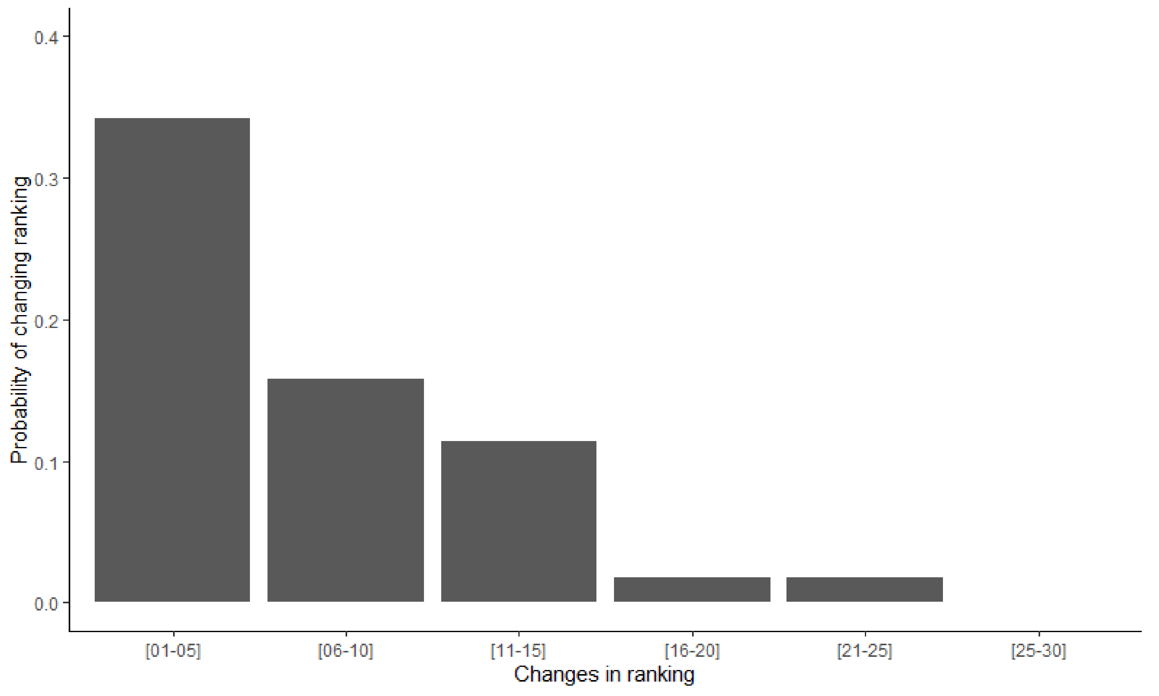
4.4. Farm Efficiency Rankings with and without Incorporating Environmental Impact

Figure 3 shows the distribution of the difference in efficiency ranking between the two models. The difference in efficiency ranking between the two models was calculated by first ranking the farm plots in descendent order given their efficiency score for each model and subtracting the ranking obtained using Model 2 (the one incorporating the environmental impact) from the ranking obtained using Model 1 (the one which does not incorporate the environmental impact). A positive value indicates that the farm plot has moved up in the ranking by the given value from using Model 1 to using Model 2, whereas a negative value indicates that the farm plot has moved down in the ranking as many places as the value obtained. Figure 3 indicates that there are changes in the ranking. Although most changes tend to be relatively small, we still find changes in ranking which are relatively large.

Examining the ranking differences between the efficiency rankings using Model 1 and Model 2, we find that 59% of the changes in efficiency level ranking from using Model 1 to Model 2 are drops in ranking and 41% are increase in rankings. Figure 4 shows the probability associated with changing ranking when accounting for environmental impact associated with N use in maize production (i.e., using Model 2) as opposed to not accounting for such impacts. For instance, the probability of ranking changing by 1 to 5 positions is 0.32. Figure 4 shows that this probability decreases as the number of changes in ranking increases.

The results obtained show that accounting for environmental impact associated with maize production matters in terms of identifying less sustainable farms. The use of satellite remote sensing data is a relatively cost-effective way of incorporating this information.

5. Discussion

Collecting environmental data at the farm/plot level requires the use of environmental surveys, smart sensors and/or reliance on farmers reporting on quantity of inputs used (e.g., K,N,P) and/or sustainable agricultural practices. Farm-level databases typically include information provided by farmers on crop and livestock data regarding production inputs used and outputs produced, using quantity and/or value units, along with farmer/household socio-demographic information. However, environmental data at the farm/plot level is usually missing from farm-level databases. One reason why this is the case may be that farm/plot level environmental information requires a substantial budget from the researchers collecting information or more effort from the farmers studied. However, if farm/plot location is available, the use of spatial environmental data can be merged with the production and socio-economic farm-level information. In this regard, satellite remote sensing data can be a cost-effective way to obtain environmental data that can be merged with farm-level data.

The results obtained show that accounting for environmental impact associated with maize production matters in terms of identifying less sustainable farms. The use of satellite remote sensing data is a relatively cost-effective way of incorporating environmental impact information into farm-level efficiency analysis.

We have shown how the use of remote sensing data (e.g., satellite data) can play a crucial role in obtaining information on environmental impact associated with agriculture production. The use of this information is crucial to develop sustainability metrics and help achieve sustainable production. Although remote sensing data obtained from satellites are available for an array of metrics, there are current limitations regarding their resolution and spatial detail outside of Europe, which limits their capabilities to be used in farm-level analysis. However, this technology is quickly advancing, and it is foreseen that this type of data will be relevant in measuring the performance of farms in producing market and environmental outputs (e.g., ecosystem services) whilst protecting the environment. For instance, although currently data on net fluxes of CO2, N2O and CH4 at earth’s surface were not available at a relevant resolution level (one pixel covers all farm plots studied) it is expected that the data resolution will improve with time. Hence, it is foreseen future research may take advantage of higher resolution earth observation data for an array of environmental impact indicators that can be used to derive environmental damage indicators. These can provide useful information that can be used in sustainability research (e.g., obtaining farm-level sustainable indicators).

Although we have demonstrated here how satellite information can help in developing novel sustainability metrics, capturing an “exact” metric for sustainability will remain a challenge. Franks (2014) [11] argues that since SI mainly serves as a boundary, stakeholders can negotiate trade-offs between agricultural production and its associated environmental impacts, meaning a precise definition of SI is not necessary. We agree that obtaining a precise/single SI metric is not possible due to the fact that SI may mean different things in different locations/environments. What is needed is a clear understanding of the interlinkages between agricultural production and the environment, and what the priorities are regarding them when developing an SI measure. It is acknowledged that the negative consequences for the environment associated with the overuse of fertilisers and poor management may be known. The authors of [34] found that costs associated with N use face large levels of uncertainty and greatly vary with management, N movements and the location, vulnerability and preferences of populations affected. The authors of [34] estimated the average social cost of N in Minnesota was $2.62 per kg N with a range between $0.44 and $10.79 per kg N. Hence, the damage function of N depends mainly on the form of N (e.g., N2O, NO and NO3) and the location [34]. When N inputs are applied in excess, there are losses of N2O, NO and NO3 to the environment, and its damage increases exponentially [34]. The interpretation of SI metrics is dependent on the choice and integration of the indicators used [12,14]. One way to moderate issues related with the choice of indicators is to maximise the use of available information. For instance, [12] used an approach where a distributional measure of SI was derived by combining the use of composite indicators with SFA. When accounting for environmental impact through any environmental impact indicator/damage function, it is important to consider spatial heterogeneity (i.e., the location), especially in studies that involve farms spread across relatively large areas/regions [35,36,37].

6. Conclusions

We have demonstrated how environmental impact indicators can be constructed from satellite data and used within a farm efficiency analysis framework to obtain sustainability indicators. We used satellite information on leaf area index to obtain a measure of environmental impact associated with N use (i.e., environmental damage). The approach used here shows how earth observation information can feed into process models that address the development of sustainability metrics by incorporating production and environmental domains into a benchmarking framework. The approach developed here can be extended in future work to account for the presence of spatial heterogeneity by bringing spatial econometric techniques in efficiency analysis.

We showed how the use of standard approaches to identify and classify farms into relative efficiency and relative inefficiency may not be appropriate if the aim is to evaluate the sustainability of the farm. The development of sustainability metrics is crucial for this aim and earth observation data can help in such development.

References

1. Ju, X.-T.; Xing, G.-X.; Chen, X.-P.; Zhang, S.-L.; Zhang, L.-J.; Liu, X.-J.; Cui, Z.-L.; Yin, B.; Christie, P.; Zhu, Z.-L.; et al. Reducing environmental risk by improving N management in intensive Chinese agricultural systems. Proc. Natl. Acad. Sci. USA 2009, 106, 3041–3046. [Google Scholar] [CrossRef] [PubMed] [Green Version]
2. Aber, J.; McDowell, W.; Nadelhoffer, K.; Magill, A.; Berntson, G.; Kamakea, M.; McNulty, S.; Currie, W.; Rustad, L.; Fernandez, I. Nitrogen Saturation in Temperate Forest Ecosystems. BioScience 1998, 48, 921–934. [Google Scholar] [CrossRef]
3. Liu, X.; Zhang, Y.; Han, W.; Tang, A.; Shen, J.; Cui, Z.; Vitousek, P.; Erisman, J.W.; Goulding, K.; Christie, P.; et al. Enhanced nitrogen deposition over China. Nature 2013, 494, 459–462. [Google Scholar] [CrossRef] [PubMed]
4. Wu, Y.; Xi, X.; Tang, X.; Luo, D.; Gu, B.; Lam, S.K.; Vitousek, P.M.; Chen, D. Policy distortions, farm size, and the overuse of agricultural chemicals in China. Proc. Natl. Acad. Sci. USA 2018, 115, 7010–7015. [Google Scholar] [CrossRef] [Green Version]
5. Liu, J.; Diamond, J. China’s environment in a globalizing world. Nature 2005, 435, 1179–1186. [Google Scholar] [CrossRef]
6. Zhu, Y.; Yao, X.; Tian, Y.; Liu, X.; Cao, W. Analysis of common canopy vegetation indices for indicating leaf nitrogen accumulations in wheat and rice. Int. J. Appl. Earth Obs. Geoinf. 2008, 10, 1–10. [Google Scholar] [CrossRef]
7. Weiss, M.; Jacob, F.; Duveiller, G. Remote sensing for agricultural applications: A meta-review. Remote Sens. Environ. 2020, 236, 111402. [Google Scholar] [CrossRef]
8. Dhillon, M.S.; Dahms, T.; Kuebert-Flock, C.; Borg, E.; Conrad, C.; Ullmann, T. Modelling Crop Biomass from Synthetic Remote Sensing Time Series: Example for the DEMMIN Test Site, Germany. Remote Sens. 2020, 12, 1819. [Google Scholar] [CrossRef]
9. Hunt, M.L.; Blackburn, G.A.; Rowland, C.S. Monitoring the Sustainable Intensification of Arable Agriculture: The Potential Role of Earth Observation. Int. J. Appl. Earth Obs. Geoinf. 2019, 81, 125–136. [Google Scholar] [CrossRef]
10. Micha, E.; Fenton, O.; Daly, K.; Kakonyi, G.; Ezzati, G.; Moloney, T.; Thornton, S. The Complex Pathway towards Farm-Level Sustainable Intensification: An Exploratory Network Analysis of Stakeholders’ Knowledge and Perception. Sustainability 2020, 12, 2578. [Google Scholar] [CrossRef] [Green Version]
11. Franks, J.R. Sustainable intensification: A UK perspective. Food Policy 2014, 47, 71–80. [Google Scholar] [CrossRef] [Green Version]
12. Areal, F.J.; Jones, P.; Mortimer, S.R.; Wilson, P. Measuring sustainable intensification: Combining composite indicators and efficiency analysis to account for positive externalities in cereal production. Land Use Policy 2018, 75, 314–326. [Google Scholar] [CrossRef] [Green Version]
13. Smith, A.; Snapp, S.; Chikowo, R.; Thorne, P.; Bekunda, M.; Glover, J. Measuring sustainable intensification in smallholder agroecosystems: A review. Glob. Food Secur. 2017, 12, 127–138. [Google Scholar] [CrossRef] [Green Version]
14. Firbank, L.G. Towards the sustainable intensification of agriculture—A systems approach to policy formulation. Front. Agric. Sci. Eng. 2020, 7, 81. [Google Scholar] [CrossRef]
15. Picazo-Tadeo, A.J.; Beltrán-Esteve, M.; Gómez-Limón, J.A. Assessing eco-efficiency with directional distance functions. Eur. J. Oper. Res. 2012, 220, 798–809. [Google Scholar] [CrossRef]
16. Faere, R.; Grosskopf, S.; Lovell, C.A.K.; Pasurka, C. Multilateral Productivity Comparisons When Some Outputs are Undesirable: A Nonparametric Approach. Rev. Econ. Stat. 1989, 71, 90. [Google Scholar] [CrossRef]
17. Färe, R.; Grosskopf, S.; Pasurka, C.A., Jr. Accounting for Air Pollution Emissions in Measures of State Manufacturing Productivity Growth. J. Reg. Sci. 2001, 41, 381–409. [Google Scholar] [CrossRef]
18. Färe, R.; Grosskopf, S.; Tyteca, D. An activity analysis model of the environmental performance of firms—Application to fossil-fuel-fired electric utilities. Ecol. Econ. 1996, 18, 161–175. [Google Scholar] [CrossRef]
19. Reinhard, S.; Lovell, C.K.; Thijssen, G. Econometric Estimation of Technical and Environmental Efficiency: An Application to Dutch Dairy Farms. Am. J. Agric. Econ. 1999, 81, 44–60. [Google Scholar] [CrossRef]
20. Reinhard, S. Nitrogen efficiency of Dutch dairy farms: A shadow cost system approach. Eur. Rev. Agric. Econ. 2000, 27, 167–186. [Google Scholar] [CrossRef]
21. Lansink, A.O.; Reinhard, S. Investigating technical efficiency and potential technological change in Dutch pig farming. Agric. Syst. 2004, 79, 353–367. [Google Scholar] [CrossRef]
22. Areal, F.J.; Tiffin, R.; Balcombe, K.G. Provision of environmental output within a multi-output distance function approach. Ecol. Econ. 2012, 78, 47–54. [Google Scholar] [CrossRef] [Green Version]
23. Omer, A.; Pascual, U.; Russell, N.P. Biodiversity Conservation and Productivity in Intensive Agricultural Systems. J. Agric. Econ. 2007, 58, 308–329. [Google Scholar] [CrossRef]
24. Gadanakis, Y.; Bennett, R.; Park, J.; Areal, F.J. Evaluating the Sustainable Intensification of arable farms. J. Environ. Manag. 2015, 150, 288–298. [Google Scholar] [CrossRef] [Green Version]
25. Ang, F.; Mortimer, S.M.; Areal, F.; Tiffin, R. On the Opportunity Cost of Crop Diversification. J. Agric. Econ. 2018, 69, 794–814. [Google Scholar] [CrossRef]
26. Elliott, J.; Firbank, L.G.; Drake, B.; Cao, Y.; Gooday, R. Exploring the Concept of Sustainable Intensification; LUPG Commissioned Report; ADAS/Firbank: Lake Orion, MI, USA, 2013; p. 187. [Google Scholar]
27. Buckwell, A.; Nordang Uhre, A.; Williams, A.; Polakova, J.; Blum, W.; Schiefer, J.; Lair, G.; Heissenhuber, A.; Schieβl, P.; Krämer, C.; et al. Sustainable Intensification of European Agriculture A review sponsored by the RISE Foundation; The RISE Foundation: Brussels, Belgium, 2014; p. 98. [Google Scholar] [CrossRef]
28. Zhao, B.; Yao, X.; Tian, Y.; Liu, X.; Ata-Ul-Karim, S.T.; Ni, J.; Cao, W.; Zhu, Y. New Critical Nitrogen Curve Based on Leaf Area Index for Winter Wheat. Agron. J. 2014, 106, 379–389. [Google Scholar] [CrossRef]
29. Zhao, B.; Ata-Ul-Karim, S.T.; Duan, A.; Liu, Z.; Wang, X.; Xiao, J.; Liu, Z.; Qin, A.; Ning, D.; Zhang, W.; et al. Determination of critical nitrogen concentration and dilution curve based on leaf area index for summer maize. Field Crop. Res. 2018, 228, 195–203. [Google Scholar] [CrossRef]
30. Zhao, B.; Ata-Ui-Karim, S.T.; Yao, X.; Tian, Y.; Cao, W.; Zhu, Y.; Liu, X. A New Curve of Critical Nitrogen Concentration Based on Spike Dry Matter for Winter Wheat in Eastern China. PLoS ONE 2016, 11, e0164545. [Google Scholar] [CrossRef]
31. Lemaire, G.; Jeuffroy, M.-H.; Gastal, F. Diagnosis tool for plant and crop N status in vegetative stage: Theory and practices for crop N management. Eur. J. Agron. 2008, 28, 614–624. [Google Scholar] [CrossRef]
32. Gelman, A.; Rubin, D.B. Infrerence from iterative simulation using multiple sequences. Stat. Sci. 2012, 7, 457–511. [Google Scholar] [CrossRef]
33. Stan Development Team. RStan: The R interface to Stan. 2020. Available online: http://mc-stan.org/ (accessed on 2 February 2022).
34. Keeler, B.L.; Gourevitch, J.D.; Polasky, S.; Isbell, F.; Tessum, C.W.; Hill, J.D.; Marshall, J.D. The social costs of nitrogen. Sci. Adv. 2016, 2, e1600219. [Google Scholar] [CrossRef] [PubMed] [Green Version]
35. Areal, F.J.; Balcombe, K.; Tiffin, R. Integrating spatial dependence into Stochastic Frontier Analysis. Aust. J. Agric. Resour. Econ. 2012, 56, 521–541. [Google Scholar] [CrossRef] [Green Version]
36. Pede, V.O.; Areal, F.J.; Singbo, A.; McKinley, J.; Kajisa, K. Spatial dependency and technical efficiency: An application of a Bayesian stochastic frontier model to irrigated and rainfed rice farmers in Bohol, Philippines. Agric. Econ. 2018, 49, 301–312. [Google Scholar] [CrossRef]
37. Areal, F.J.; Pede, V.O. Modeling Spatial Interaction in Stochastic Frontier Analysis. Front. Sustain. Food Syst. 2021, 5, 5. [Google Scholar] [CrossRef]
Figure 1. Location area of maize farms.
Sustainability 14 01832 g001
Figure 2. Conditional posterior distributions for mean efficiency across maize farms for models M1 and M2.
Sustainability 14 01832 g002
Figure 3. Efficiency ranking differences between Model 1 and Model 2.
Sustainability 14 01832 g003
Figure 4. Probability of ranking changing by (1–5), (6–10), (11–15), (16–20), (21–25) and (25–30) positions.
Sustainability 14 01832 g004