An Integrated Approach for Evaluating Climate Change Risks: A Case Study in Suriname

Abstract

This paper combines long-term state-of-the-art climate projections and indices to provide detailed insights into the future climate of Suriname to facilitate comprehensive information of areas and sectors at high climate risk for political decision-making. The study analyses Suriname’s historical climate (1990–2014) and provides climate projections for three time horizons (2020–2044, 2045–2069, 2070–2094) and two emissions scenarios (intermediate/SSP2-4.5 and severe/SSP5-8.5). Coupled Model Intercomparison Project (CMIP6) modeling is used to analyze changes in sea level, temperature, precipitation, relative humidity, and winds. In addition, risk impact chains were produced for the country’s four most important socio-economic sectors: agriculture and fisheries, forestry, water, and infrastructure. Results show the temperature is expected to increase for all regions and timeframes, reaching warming up to 6 °C in the southern region in the long-term future (2070–2094). Projections point towards a reduction in precipitation in the southwest and coastal regions and a rise in mean sea level. Regarding risk, Paramaribo and Wanica face the highest climate risk. Coronie and Nickerie face the least climate risk. These regions remain the most and least vulnerable in both the SSP2-4.5 and SSP5-8.5 scenarios, but overall values of their risk indices increase substantially over time.

1. Introduction

Small Island Developing States (SIDS) are highly vulnerable to climate change-related hazards. Mostly situated in the tropics, SIDS are struck by thunderstorms, cyclones, lightning, coastal storm surges, intense rainfall resulting in coastal and inland flooding, droughts, damaging winds, and heatwaves, among others [1,2,3,4]. These hazards can severely impact vulnerable and exposed populations and infrastructure in SIDS, resulting in loss of life, destruction to infrastructure and livelihoods, and causing, e.g., coastal erosion, epidemics, and landslides. Such events have negatively affected the socio-economic development of already fragile SIDS economies, which often have limited development opportunities, in many cases associated with tourism development, and are sensitive to external macroeconomic shocks [5,6]. They are largely reliant on local markets, subsistence farming, fisheries, and natural resources to maintain livelihoods. In the near future, climate change is likely to increase the frequency and severity of such hazards in these territories while simultaneously increasing their vulnerability by damaging ecosystems and limiting traditional livelihoods [4,6].

This is the case with Suriname [7,8]. The country’s small population, infrastructure, and major economic activities are concentrated along the low-lying coastal zone, which has already experienced considerable coastal erosion and damages from heavy rainfall and rising temperatures [9]. About 80% of the total population lives along the coastline [10]. This elevated exposure to natural hazards creates fiscal and macroeconomic stability risks, private investment in productive activities, sustainable growth, and poverty reduction.

Research has previously been conducted regarding forecasting and projections under IPCC AR4 and AR5 [11,12]. However, further studies were necessary to consolidate historical data, improve the resolution of projections, update existing research, and translate scientific data into manageable information for policy purposes and economic and social decision-making.

This article proposes a holistic methodology to assess Suriname’s climate risk. First, the study analyses Suriname’s historical climate (1990–2014) and provides climate projections for three time horizons (2020–2044, 2045–2069, 2070–2094) and two emissions scenarios (intermediate/SSP2-4.5 and severe/SSP5-8.5). This analysis focuses on changes in sea level, temperature, precipitation, relative humidity, and winds. Through a grid level for the entire national territory, the results inform on the possible future development of natural hazards at the country and district-level, and at seven discrete subnational points of interest, namely Paramaribo, Albina, Bigi Pan Multiple Use Management Area (MUMA), Brokopondo, Kwamalasamutu, Tafelberg Natural Reserve, and Upper Tapanahony. Second, the article also analyses climate risk for the country’s ten administrative districts by additionally examining the factors which increase influence their populations’ and ecosystems’ exposure and vulnerability in and across the four most important socio-economic sectors affected by climate change: infrastructure, agriculture, water, and forestry. Thus, the results provide a thoroughly scientific basis for developing and updating Suriname’s climate change policies and targets. These policies and targets should enable an adequate mainstreaming of climate change adaptation and resilience enhancement into day-to-day government operations.

Therefore, the overall goal of the paper is to improve climate change decision-making in the country by providing solid science-based evidence on expected climate impacts and a quantitative risk assessment that considers geographical and sectoral issues. The paper is structured as follows: Section 2 gives an overview of the methodology. Section 3 summarizes the projection results and the reanalysis of historical data. Section 4 delves into the risk assessment and its main components. Section 5 focuses on the discussion of the methodology and results. Finally, the paper finishes with some concluding remarks.

2. Materials and Methods

The methodology of this research can be summarized into two main steps:

• Analyzing the historical climate, identifying trends, and developing climate projections.
• Conducting a risk assessment by analyzing cause-effect relationships, quantifying them with indicators and summarizing them into indices.

Three climate models from the framework of the CMIP6 were used. HadGEM3-GC31 and MIROC6 were selected due to their satisfactory precipitation and atmospheric simulation in the monsoon-affected areas with Amazonian characteristics. Examples of these applications were found in the literature [13] for Brazil, whose north has the same Köppen classification as the study area, namely areas classified as equatorial forests or fully humid areas (Af) and equatorial monsoon areas (Am) [14] IPSL-CM6A was included, due to suggestions from local experts. The ensemble of these models was used due to the models’ climate sensitivity. Climate sensitivity is calculated with the average change in the planet’s surface temperature in response to changes in radiative forcing. Each has very different climate sensitivity ranges, with HadGEM3-GC31 having the highest climate sensitivity and MIROC6 the lowest, and IPSL-CM6A can be located in a medium climate sensitivity range. Altogether, the three models cover a wide range of climate sensitivities, as shown in

Table 1. CMIP6 CGMs used in the multi-model approach and their corresponding climate sensitivity. Source: own elaboration.

GCM Acronym	Centre	Climate Sensitivity
HadGEM3-GC31	Met Office Hadley Centre for Climate Change	High
MIROC6	Atmosphere and Ocean Research Institute (AORI), Centre for Climate System Research—National Institute for Environmental Studies (CCSR-NIES)	Low
IPSL-CM6A	Institute Pierre-Simon Laplace (IPSL)	Medium

.

For the last available IPCC assessment report, Representative Concentration Pathways (RCP) were developed, based on an approximate calculation of the total radiative forcing in the year 2100 in relation to 1750, which can be 2.6 Wm⁻² (RCP2.6 scenario), 4.5 Wm⁻² (SSP2-4.5 scenario), 6.0 Wm⁻² (RCP2.6 scenario) or 8.5 Wm⁻² (RCP2.6 scenario). Within Phase 6 of the CMIP6, these scenarios have been accompanied by a socio-economic narrative. For this purpose, Shared Socio-Economic Pathways (SSP) were defined [15]. These Shared Socio-Economic Pathways (SSPs) discuss five different ways in which the world could evolve in the absence of climate policy: a world of growth and equality focused on sustainability (SSP1); a middle-of-the-road world in which trends broadly follow their historical patterns (SSP2); a fragmented world of “resurgent nationalism” (SSP3); a world of growing inequality (SSP4); and a world of rapid and unconstrained growth in economic production and energy use (SSP5). These narratives describe alternative pathways for future society [16]. Scenarios SSP2-4.5 and SSP5-8.5 were selected for the climate projections [17]. Statistical downscaling was conducted using the quantile-quantile adjustment method (Q-Q) [18,19]. This method corrects the projections according to the differences between the simulated climatic parameters in the future and present scenarios, the errors in the mean, and the variability and the distribution of the future climatic variables.

For the projections, 25-year periods were defined to have three future periods: 2020–2044, 2045–2069 and 2070–2094. In line herewith, a reference period of 25 years from 1 January 1990 to 31 December 2014 was used.

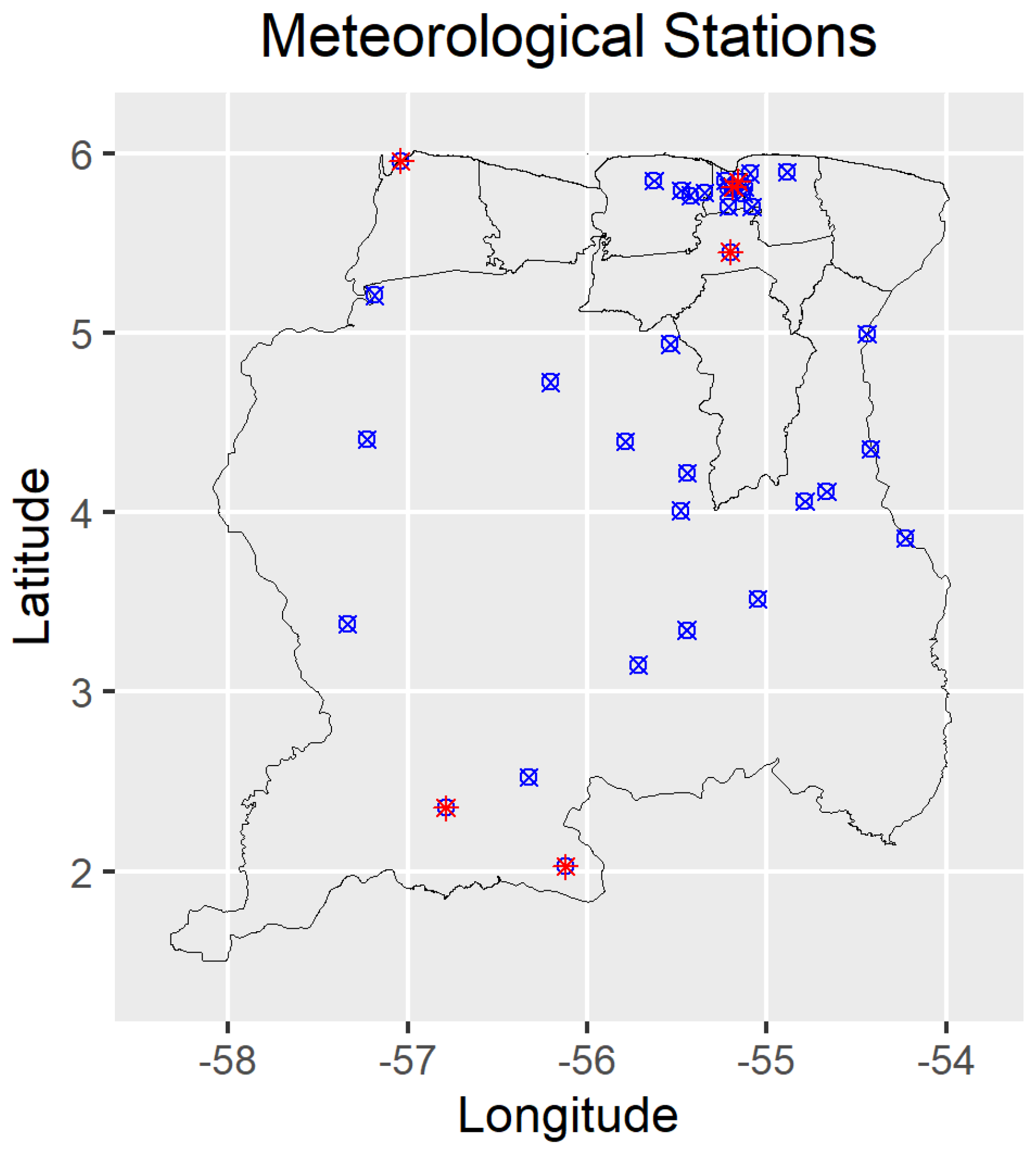
The Meteorological Service of Suriname provided the daily historical data for 35 stations from 1990 to 2019 (Figure 1). The analysis of this dataset was especially challenging, due to time series and data limitations. The data set from Suriname was used to calibrate the historical data provided by ERA5, which covers the entire country at a spatial resolution of 0.25° with temporal continuity, except for ERA5 wind observations, which could not be used.

The probability matching technique was used [20], so the probability of events in the reanalysis data was matched with that of the observed data.

Table 2. Variables/Indices used and their description and unit. Source: own elaboration based on expert criteria and other studies [24,25,26,27].

Abbreviation	Variable/Index	Description	Units
tmean	Variable	Average daily temperature	°C
tmax	Variable	Maximum daily temperature	°C
tmin	Variable	Minimum daily temperature	°C
TX90	index	Days on which the mean temperature exceeds the mean temperature of 10% of the hottest days	days/year
TX10	index	Days on which the mean temperature drops below the mean temperature of 10% of the coldest days	days/year
TN90	index	Nights in which the mean temperature does not reach the mean temperature of 10% of the hottest nights	days/year
TN10	index	Nights in which the mean temperature drops below the mean temperature of 10% of the coldest nights	days/year
Accumulated pcp	Variable	Accumulated precipitation	mm/year
Rainy days	index	Number of days with more than 1 mm of rain	days/year
RX1day	index	Value of maximum accumulated precipitation in 1 day	mm
RX5day	index	Value of maximum accumulated precipitation in 5 days	mm
Maximum wind	Variable	Average of maximum daily wind	Km/h
Strong wind days	index	Number of days with maximum wind stronger than 40 km/h and lower or equal to 60 km/h	days/year
Gale wind days	index	Number of days with maximum wind stronger than 60 km/h	days/year
SLA	Variable	Increase of sea level above sea height	m
Humidity	Variable	Average relative humidity	%

details the variables and indices analyzed in the study. Although not usual in climate studies, the wind variable and some indices have been included. Wind is necessary for more detailed impact studies because of the large geophysical and social impacts of changes in this variable [21]. Some of the possible impacts of changes in the wind may be, for example, impacts on the mortality of patients with asthma and other respiratory diseases [22] or the capacity for renewable energy development such as wind energy [23].

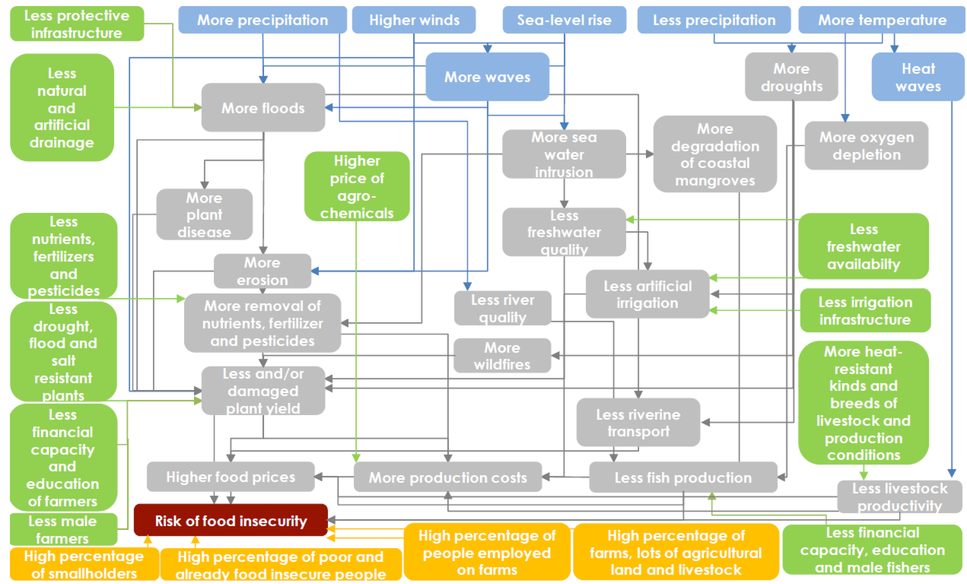
The risk was defined as the product of hazards, exposure and vulnerability [28]. Based on expert opinion and a literature review, impact chains were produced for the country’s four most important socio-economic sectors: agriculture and fisheries, forestry, water, and infrastructure (energy, transport, and buildings). An example of this approach for the agricultural sector is shown in Figure 2).

Impact chains are powerful tools to visualize cause-effect relationships. However, their interpretation is complex, and unlike risk indices, they are weak in terms of mathematical foundations [29].

Thus, risk indices were elaborated based on the factors and elements identified with the impact chains, data produced in the climate analysis, and a standard five-step procedure [30,31].

• Indicator selection. Based on the definition of risk and the available data, 19 indicators representing hazards (Table 2, excluding SLA but including additional indicators on dry, short dry, rainy, and short rainy season precipitation), 20 indicators for exposure and 13 indicators for vulnerability with data disaggregated at the district level were selected across the four sectors (see Supplementary Materials). The hazard indicators were available for the historical period (1990–2014), short-term (2020–2044), mid-term (2045–2069), and long-term (2070–2094) future, and the emission scenarios SSP2-4.5 and SSP5-8.5.
• Data quality control. Then, the indicators were screened and corrected for outliers, missing data and correlation.
• Normalization. The minimum-maximum normalization was applied to the indicators in Table 2 (hazard indicators) and the Supplementary Materials (exposure and vulnerability indicators), yielding values on a range of 1–2 (Equation (1)).

  $$x_{normalized}=\frac{x-mi{n}_x}{ma{x}_x-mi{n}_x}+1$$

  (1)

  where:
  • x_normalized: normalized value on a range of 1–2
  • x_min: minimum value of the entire dataset (historical data and six projections)
  • x_max: maximum value of the dataset (historical data and six projections)

The indicators in Table 2 and the Supplementary Materials were also inverted where necessary, so higher values correspond to greater hazards, exposure, vulnerability and risk (Equation (2)) (for the hazard indicators in Table 2, this was the case for TX10, TN10, accumulated precipitation and rainy days). The inversion conserves the range of values between 1–2.

$$x_{inverted}=3-x_{normalized}$$

(2)

where:

• x_inverted: inverted value (the higher, the greater the hazard/exposure/vulnerability/risk index)
• x_normalized: normalized value on a range of 1–2

4.

Weights. Using equal weights, the indicators were aggregated into their respective sub-indices for hazards, exposure and vulnerability. The different numbers of indicators in the sub-indices were accounted for according to the following formula (Equation (3)):

$$SI=I_1{}^{1/n}\times I_2{}^{1/n}\times \dots \times I_n{}^{1/n}$$

(3)

where:

• SI: sub-index
• I_1–n: indicators
• n: number of indicators

When aggregating the sub-indices into the risk index, the hazard sub-index was given double the weight in comparison to the vulnerability or exposure sub-indices (Equation (4)):

$$R=H^{1/2}\times E^{1/4}\times V^{1/4}$$

(4)

where:

• R: Risk index
• H: Hazard sub-index
• E: Exposure sub-index
• V: Vulnerability sub-index

5.

Aggregation. Multiplication was used for aggregation for all indices (see the previous step).

3. Development of Climate Projections

The development of climate projection analysis is based on comparing between different future periods and a so-called historical or reference period. For this reason, the first step is to characterize the reference period as accurately as possible. The next step consists of analyzing climate projections calibrated and compared with the reference period.

3.1. Reference Period

The aim of the reference period is to analyze the historical climate to subsequently elaborate future climate projections. The modelling of observations plays an important role in this type of study. These observations constitute the climate of the present time, allowing us to see what the trends are and how they differ from the future climate. In addition, this period is also used for the initialization of climate projections using the Q-Q technique [18,19]. All this means that the modelling of the present climate has to be correctly regionalized to obtain precise projections. The use of station data exclusively would lead to gaps in the region’s grid and, therefore, it would be impossible to model the different variables correctly. On the other hand, using only reanalysis simulated observations over the whole territory, there would be slight deviations at high resolution. Using the probability matching technique [20], the reanalysis grid can be adjusted to the observations of the site providing a much more reliable downscaling technique than using only one data source. This reference period is based on the results obtained from the ERA5 reanalysis data calibrated with in-situ observations for three variables: precipitation, temperature, and relative humidity. No observations were available for the wind and sea level, so reanalysis data have been used. Furthermore, in the case of sea level, only reanalysis data are used because there are no reliable tide gauge data in the area due to the characteristics of the coastline, consisting of beaches and mangroves. This type of coastline has short and very short-term variability and terrain displacement, making observation unreliable. In this situation, sensors are not usually installed to make observations. Instead of dealing with the sea level variable, the sea level rise variable has been studied for all these reasons. This variable makes it possible to carry out a general study to define the risks to anticipate possible risks, considering the reliability of the occurrence of the phenomena and the current state. Therefore, the sea level rise variable has been calculated between periods by using the mean sea level for each period and studying the difference between them to represent the sea level rise variable.

3.1.1. Region Analysis

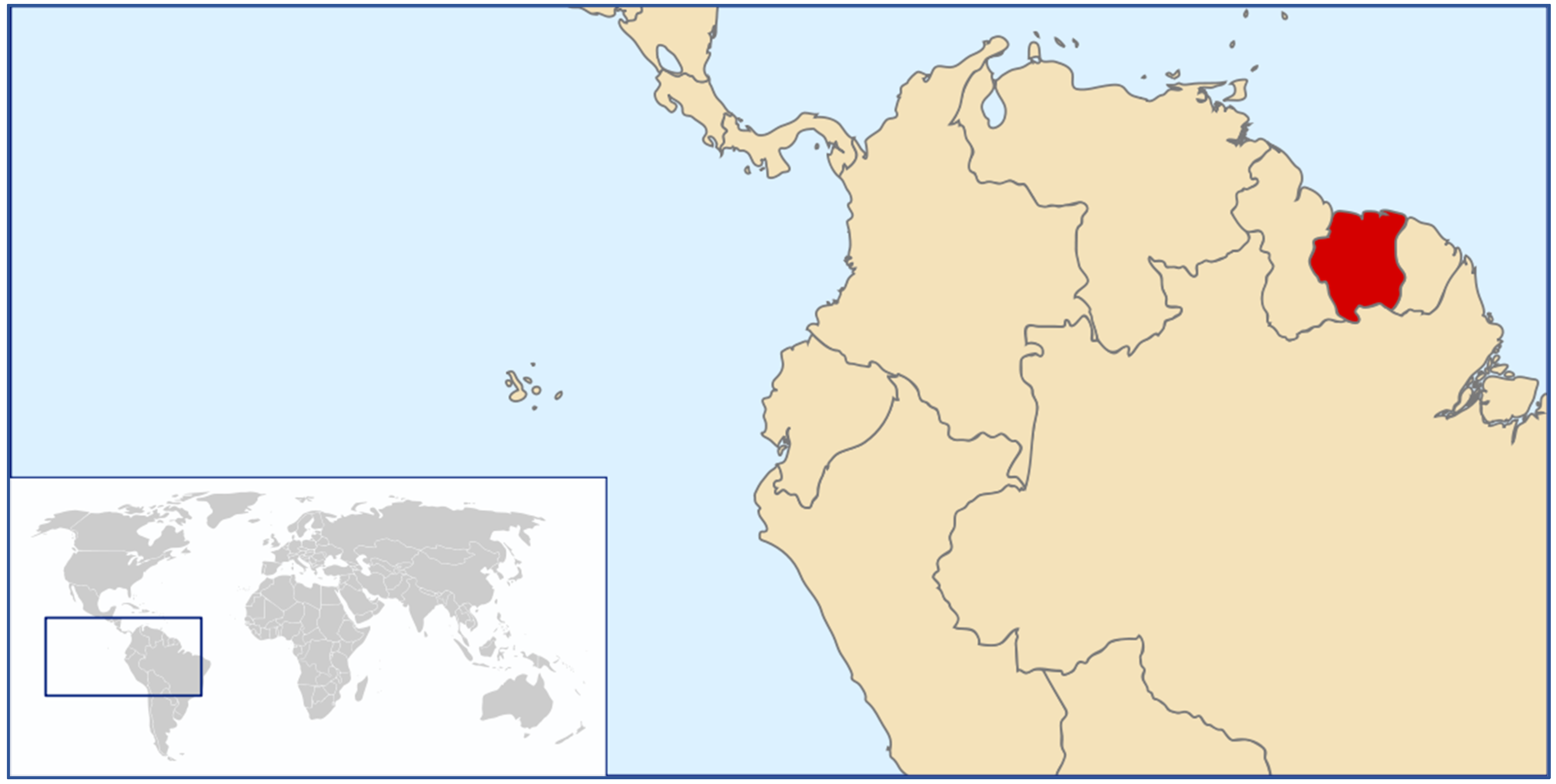
Suriname is located at the north of the equator on the northeastern coast of South America between 40–60 north latitude and 54–58 west longitude (Figure 3). According to the latest update of the Köppen-Geiger climate classification Suriname has a tropical climate [14], with abundant rainfall, uniform temperature and high humidity. The country shows a smooth topography, with height ascending as one moves southwards from the only coast in the north. This slight variation in altitude leads to diverging coastal and interior climates. The topography of the country’s northern half is composed of a flat coastal plain and low hills further inland. The overall pattern of the hinterland, the southern half of the country, is composed of the central highlands, with a few locations rising to slightly over 1000 m above sea-level [32].

3.1.2. Temperature Results

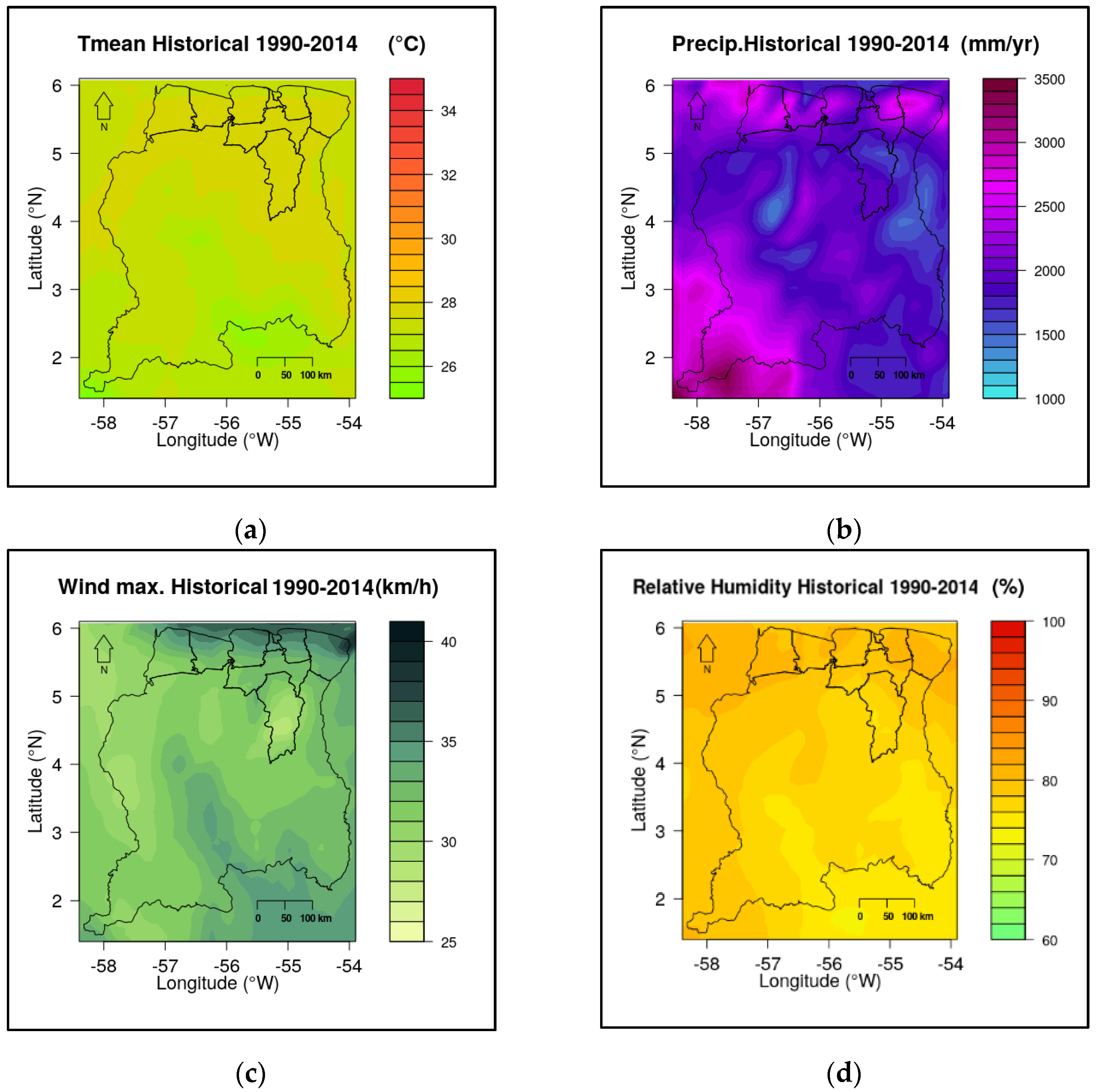
The average daily temperature in the coastal region is 27.6 °C, with an average daily variation of 4 °C. There is relatively little variation in temperatures between the seasons in the coastal region (see spatial distribution in Figure 4a). January is the coldest month (with an average temperature of 27.5 °C) and October is the warmest (with an average temperature of 29.2 °C). Thus, the annual variation of the average temperature is 2–3 °C. The interior has a relatively similar pattern, with an even smaller annual variation of average temperatures.

In addition to the description of the variables, indices have also been calculated to identify risks to the population. In the case of temperature, these indices are based on the 10th and 90th percentiles of daily maximum and minimum temperatures. For the reference period, the frequency of cool days and nights was around 40 days per year. The frequency of warm days and nights was around 50 days per year.

3.1.3. Rainfall Results

Precipitation amounts vary across the country (see spatial distribution in Figure 4b). On average, Paramaribo receives 1756 mm of rainfall annually; Bigi Pan (north-western coast) receives 1796 mm/year; Kwamalasamutu (southern Suriname) 2392 mm/year and Tafelberg (central Suriname) 1851 mm/year. Variation in monthly rainfall results in two wet and two dry seasons in the northern part of Suriname. In the south, only one wet and one dry season are distinguished.

3.1.4. Wind Results

Although unusual in climate studies, the wind variable and some indices have been included, given some studies showing significant changes in the distribution of wind speed worldwide [33] and the large geophysical and social impacts [34] that these changes can produce.

Winds in Suriname generally move in a north-easterly direction. Maximum average wind speed ranges from 30–42 km/h on the coast to about 30 km/h in the interior. The highest wind speeds are reached during the dry seasons, with up to 40 km/h in March and a second stronger peak in September and October. Wind speeds are relatively high along with coastal areas and decrease as one moves inland (see spatial distribution in Figure 4c). Wind speeds of 70 to 110 km/h generally occur during the day and drop dramatically during the evening and night, especially in the interior.

Although Suriname lies outside the hurricane belt, the country’s weather is occasionally affected by the outward bands of hurricane winds. Local gales (called Sibibusi) occur before storms, generally at the end of the rainy seasons. During such gales, maximum wind speeds of 20–30 m/s have been recorded. Such gales occur over the entire country and may destroy trees and houses. This happens on less than three days a year. Strong winds are more frequent and can happen up to 100 days a year in the coastal region.

3.1.5. Humidity Results

It is not common to use the relative humidity variable in climate studies, so it is important to highlight that humidity can impact, for instance, mortality [35] or cloud cover [36].

Daily air humidity is on average 80–90% in the coastal regions. It is lower in the central and southern regions of the country, with an average of 75% (see spatial distribution in Figure 4d). In forested areas, air humidity depends, among other things, on the penetration of solar radiation. Relative air humidity ranges between 70 to 100% in forested areas, and between 50 to 100% in open areas.

3.2. Future Periods

The most relevant results of this work regarding future climate scenarios for Suriname concern two main variables: temperature and rainfall. The rest of the variables (wind and relative humidity and their derived indices) show little or no change and are therefore of less interest.

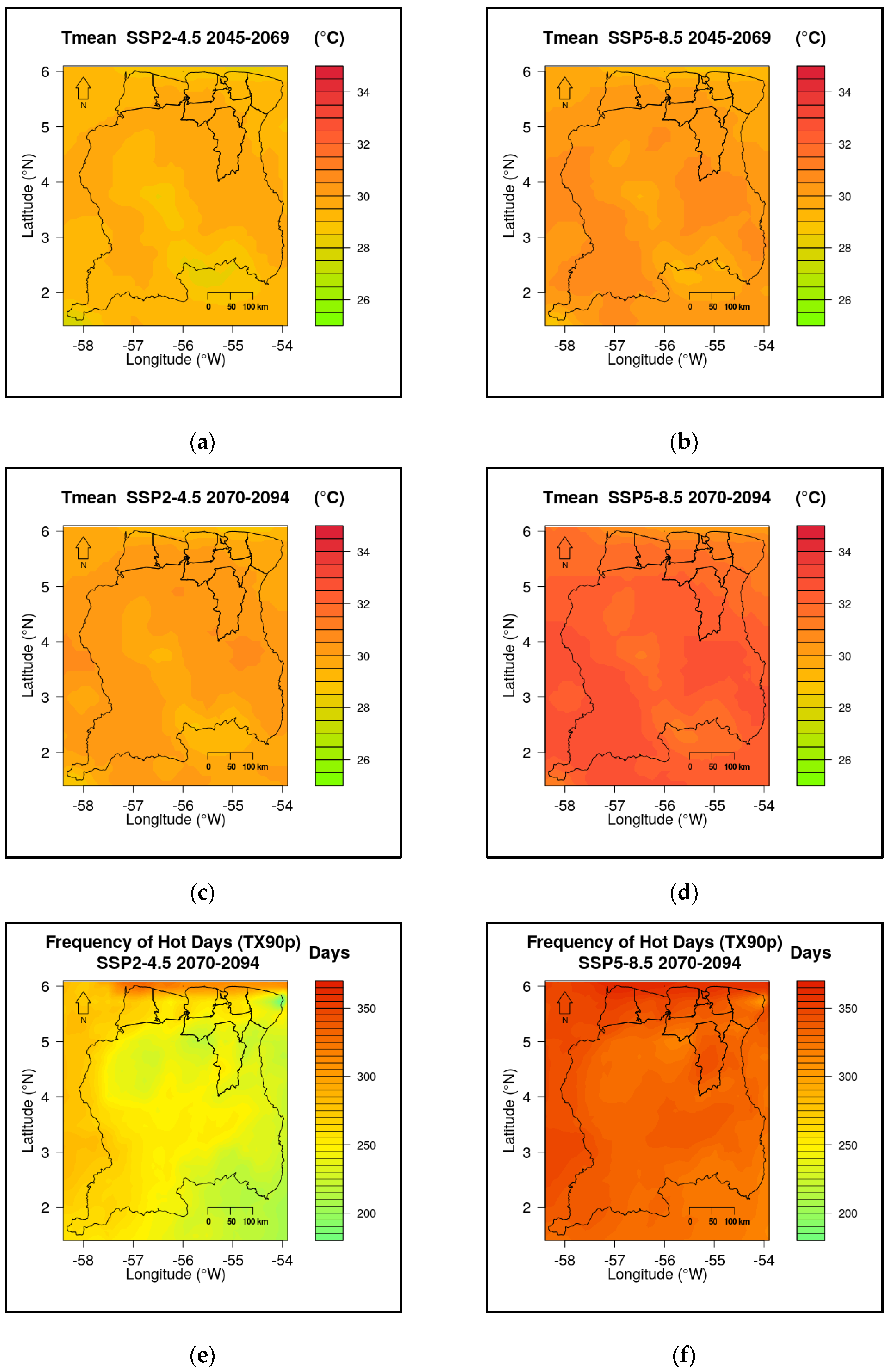
3.2.1. Temperature Projections

Temperature is expected to increase throughout the country, for all regions and timeframes. In the short-term future, maximum and minimum temperatures show a slight increase, which is stronger in the southern part of the country. This pattern is enhanced in the SSP5-8.5 scenario compared to the SSP2-4.5 scenario (Figure 5a–d). This pattern is evident when comparing the values for the long future in the SSP2-4.5 scenario (Figure 5c) with the values for the short future in the SSP5-8.5 scenario (Figure 5b), where the values exceed the previous one by around 1.5 °C. Temperature constantly increases over time, reaching a warming of up to 6 °C, above the current average temperature (Figure 4a), in the southern region for the long-term future (2070–2094). This increase is particularly strong during the dry season, when the maximum temperature is reached. Extreme indices, which depend on temperature, are projected to change as well, with the frequency of cold days falling sharply to zero by the end of the century, and hot days and nights reaching almost 90% of the total (Figure 5e,f).

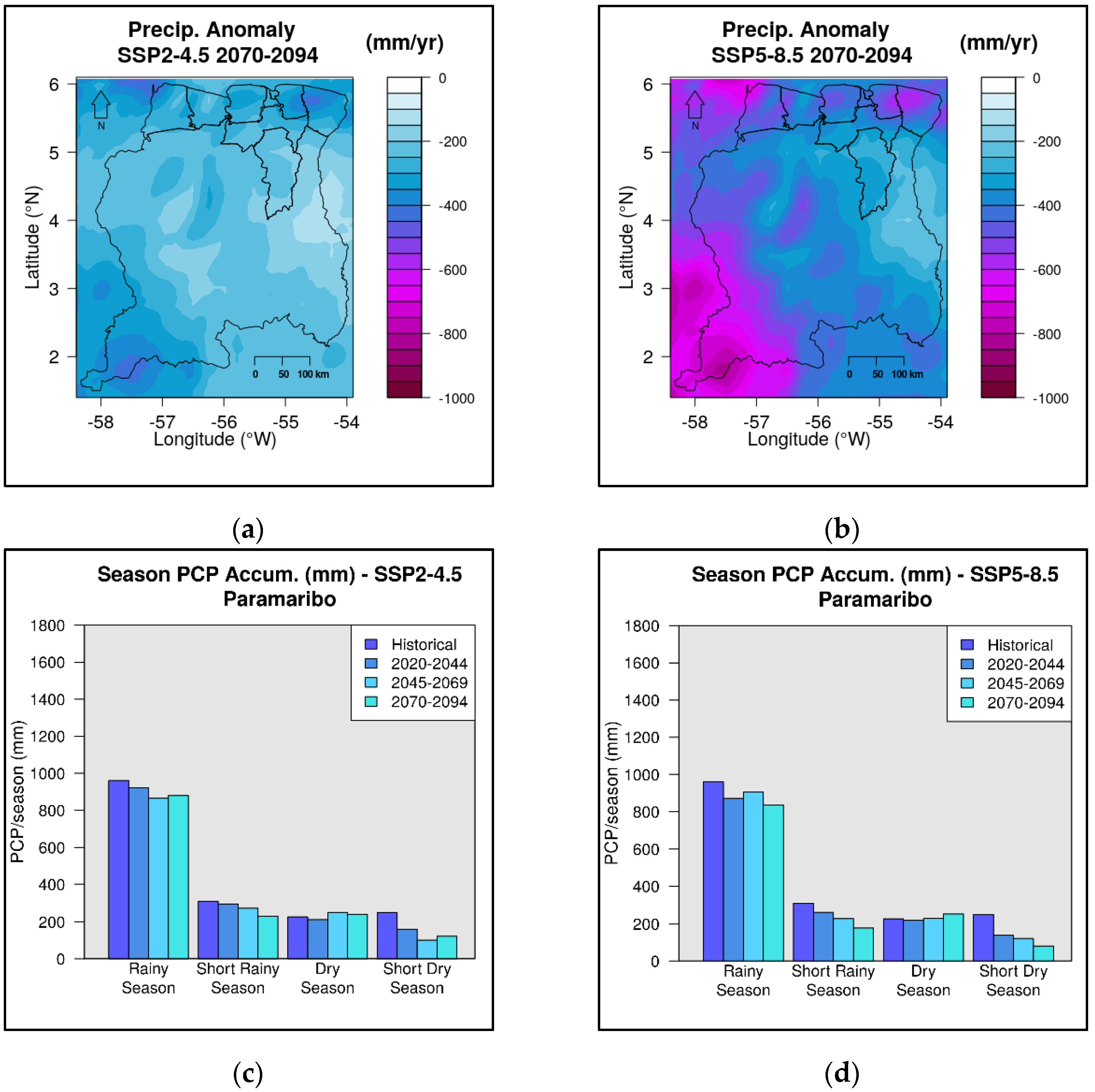
3.2.2. Rainfall Projections

Rainy days and accumulated precipitation are also expected to decrease more strongly in the southwest and coastal regions than in the inner part of the country. The effects are gradual (with accumulated precipitation decreasing to 300 mm/year for the short-term and to 600 mm/year in the long-term for the SSP2-4.5 scenario), with a much larger reduction under the SSP5-8.5 scenario (Figure 6a,b). However, the most relevant change to precipitation is not its decrease but the changes in its temporal distribution. In the coastal regions, the dry season is expected to become wetter. In contrast, the rainy season is expected to become drier. In the interior, the short dry season might become much drier (this effect is clear in both RCPs scenarios and in the short-term), while the rainy season is expected to become considerably wetter in the short-term. A slightly wetter season is expected in the long-term in the SSP5-8.5 scenario for this region (Figure 6c,d).

The change in the seasonality of rain might be related to changes in the ITCZ seasonal cycle, which is projected to be shorter over Suriname. The most obvious consequence is that the precipitation distribution in the southern part of the country is expected to become less smooth, with the rainy season concentrated in fewer months. This leads to a decrease in the number of rainy days and an increase in extreme precipitation episodes.

As for the calculated rainfall indices, in both cases, both for the maximum rainfall in one day (RX1day), and for the maximum rainfall in five consecutive days (RX5days) the amount of rainfall is expected to increase in comparison to the data of the reference period. Rainfall episodes will thus be less frequent but more severe.

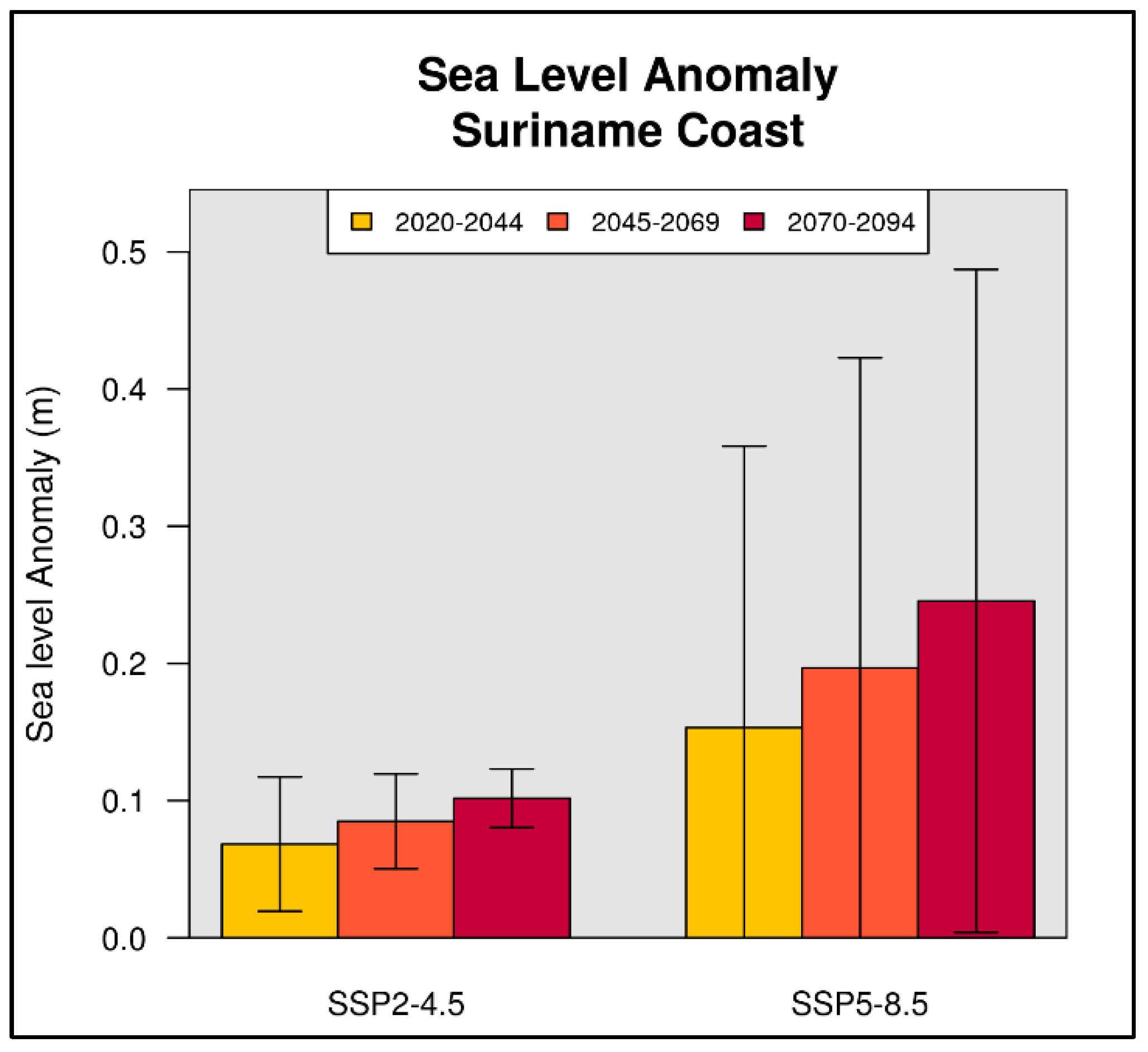
3.2.3. Sea-Level Projections

Mean sea level is expected to gradually rise by about 1 cm per decade in the SSP2-4.5 scenario, reaching almost one meter in the long-term future. According to the SSP5-8.5 scenario, the rate of sea-level rise would be 2.5 times this value, reaching 2.5 cm per decade in the far future. However, the uncertainty involved in quantifying sea level rise is greater than in any other analyzed variables (Figure 7). While the general trend is robust, the projected sea level anomaly that will be reached is not so clear. More research is needed to get a better description of this variable.

4. Risk Assessment

First, the individual components of risk, namely, hazard, exposure and vulnerability sub-indices, including the indicators that composed them, were analyzed. Subsequently, risk as the product of these three components was evaluated.

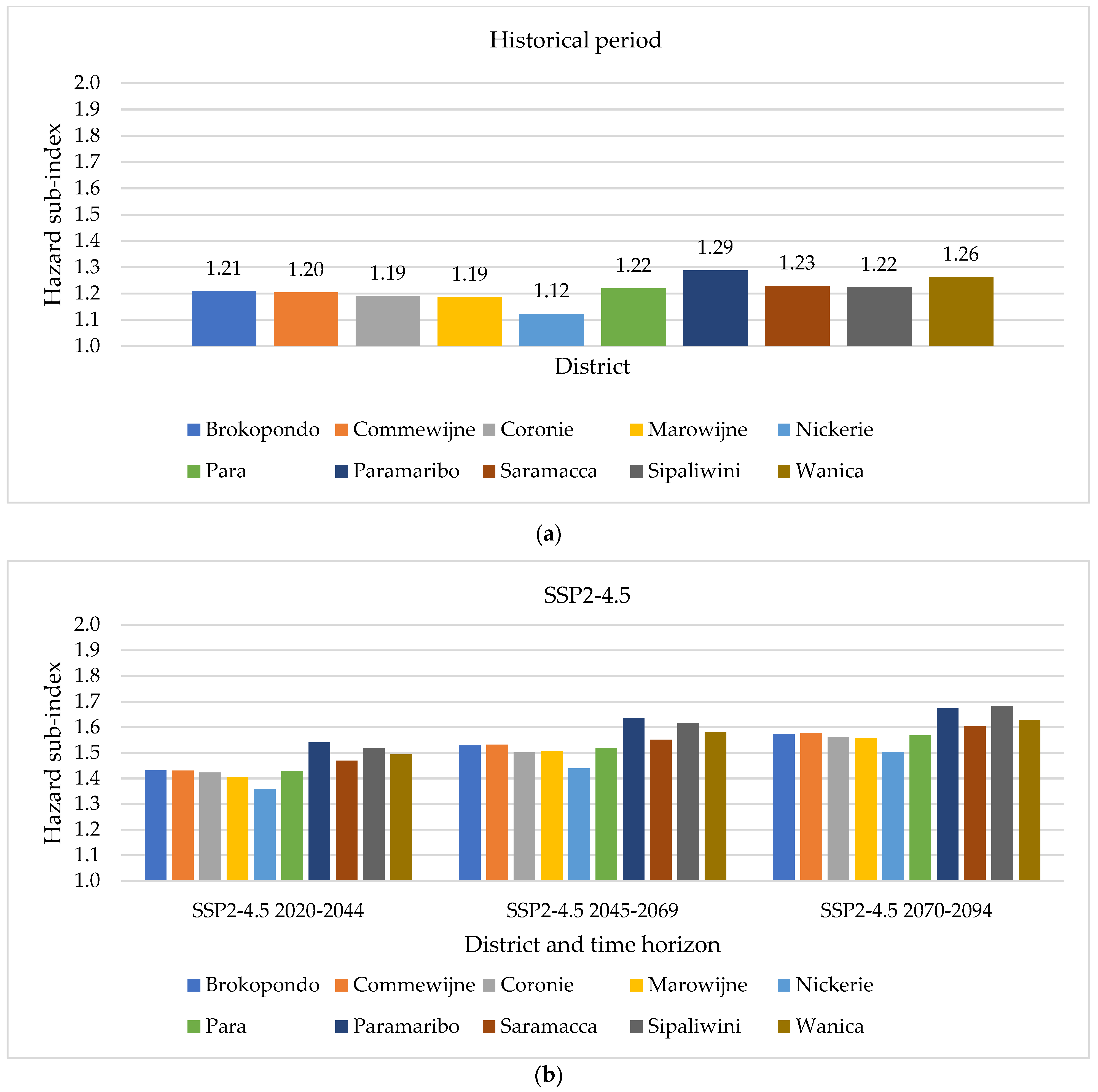
4.1. Hazards

For the historical period, Paramaribo yielded the highest hazard sub-index, followed by Wanica. Nickerie, by far, scored the lowest (Figure 8a).

In the SSP2-4.5 scenario, all districts’ sub-indices increased by at least 17.1% (Figure 8). Paramaribo remained the highest scoring district in the short- and mid-term. Nickerie remained the lowest-scoring district throughout, despite its sub-index increasing by 21.1-33.8%. Only Sipaliwini’s sub-index increased more (24.0–37.6%). Accordingly, Sipaliwini shot to the top of the ranking, outscoring Wanica already in the short term, and Paramaribo in the long term.

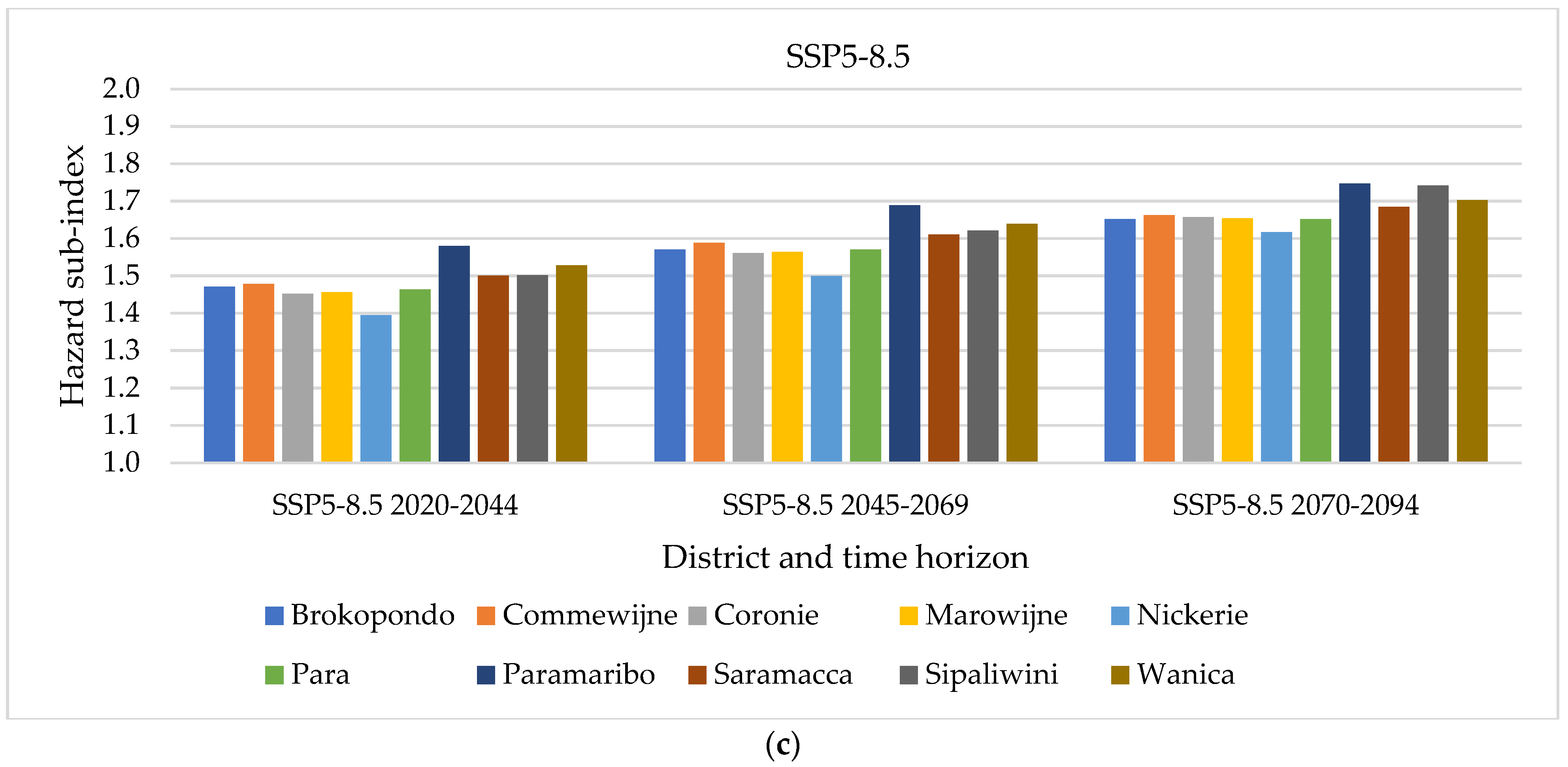
In the SSP5-8.5 scenario, all districts’ sub-indices increased by at least 19.9% (Figure 8c). Paramaribo and Nickerie remained the districts with the highest and lowest sub-indices, respectively. In this scenario, Nickerie’ s hazard sub-index increased by 24.2–44.0%, more than in any other district and the SSP2-4.5 scenario. Again, Sipaliwini’ s sub-index also witnessed a high increase (22.7–42.3%), particularly in the long-term, where Sipaliwini outscored Wanica.

The district whose sub-index changes the least in both scenarios is Para, facing increases of only 17.1–28.6% in the SSP2-4.5 scenario and 19.9–35.4% in the SSP5-8.5 scenario.

Regarding the single hazard indicators (considering some were inverted so that increases corresponded to a higher hazard), all those based on temperature increase over time under more severe climate scenarios, particularly the indicators on the frequency of cold days, cold and hot nights. In the SSP5-8.5 scenarios the indicator on the frequency of hot days also increased substantially in the long term. However, Sipaliwini’ s hazard sub-index change is related to sharp increases in maximum, average, and minimum temperature. The district scored the highest increases of all districts throughout all scenarios and timeframes.

Almost all hazard indicators on precipitation increased over time under more severe climate scenarios, particularly the indicator on maximum precipitation in five days. The only exception is the indicator on dry season precipitation, which decreased in all districts apart from Sipaliwini. A beneficial development of the indicators on maximum precipitation in one day was also observed in the SSP2-4.5 scenario in the short term for most districts. Still the indicator later increased in the mid and long term in both scenarios. The development of Sipaliwini’ s sub-index was also driven by changes in the short dry season precipitation indicator.

The indicators on gale winds did not change for any district but Sipaliwini. The indicator on maximum wind speed increased slightly, and the indicator on the number of days with strong winds increased or decreased slightly, depending on the district. The relative humidity indicator decreased across timeframes and scenarios, particularly for Sipaliwini and Brokopondo.

4.2. Exposure

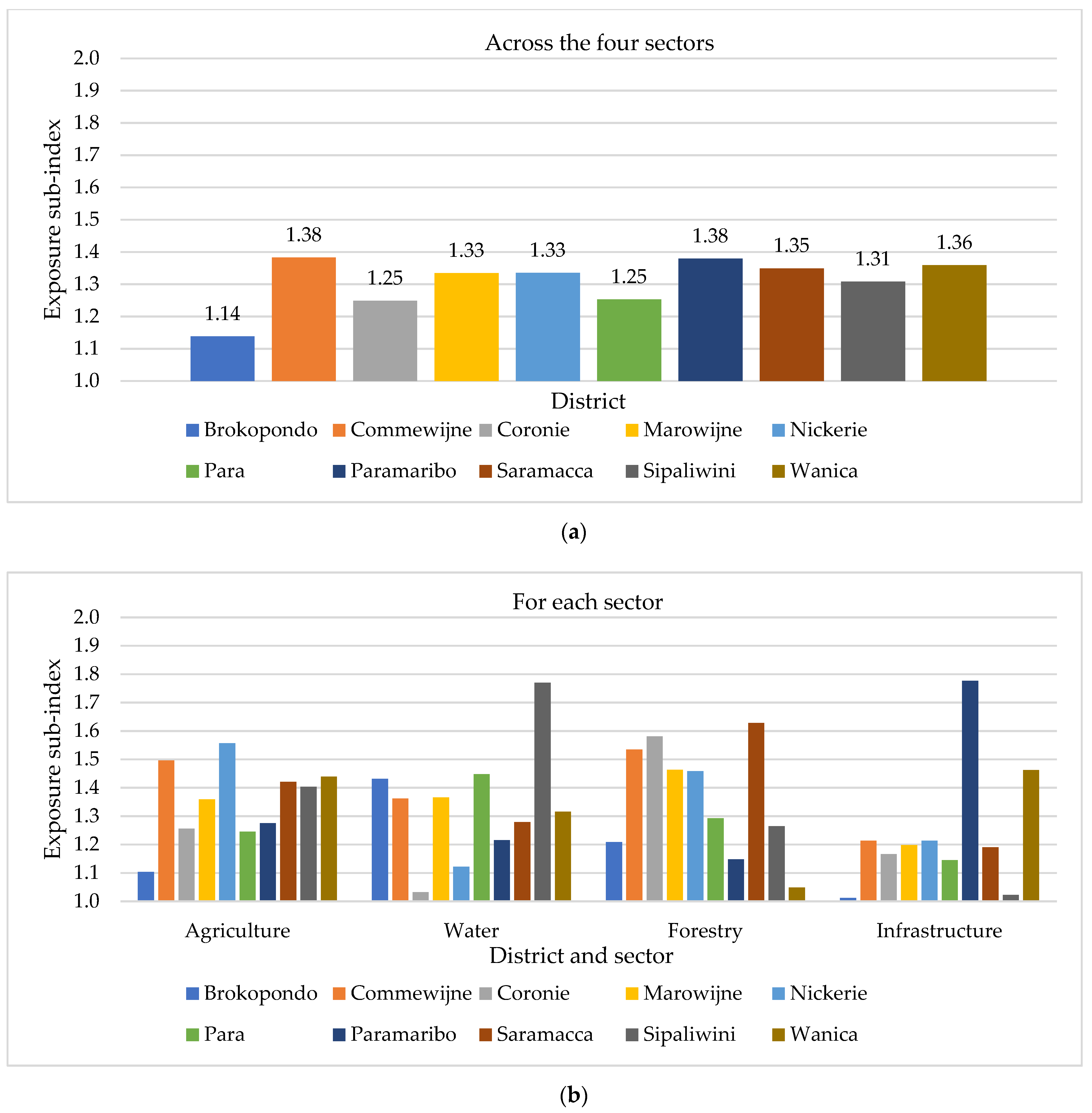
Commewijne and Paramaribo were the most exposed districts, and Brokopondo was the least exposed district (Figure 9a). Commewijne demonstrated a great exposure in agriculture, water and forestry (Figure 9b). Paramaribo had by far the highest exposure in infrastructure. Brokopondo scores very low for agriculture and infrastructure, with elevated and medium exposure values in water and forestry.

4.3. Vulnerability

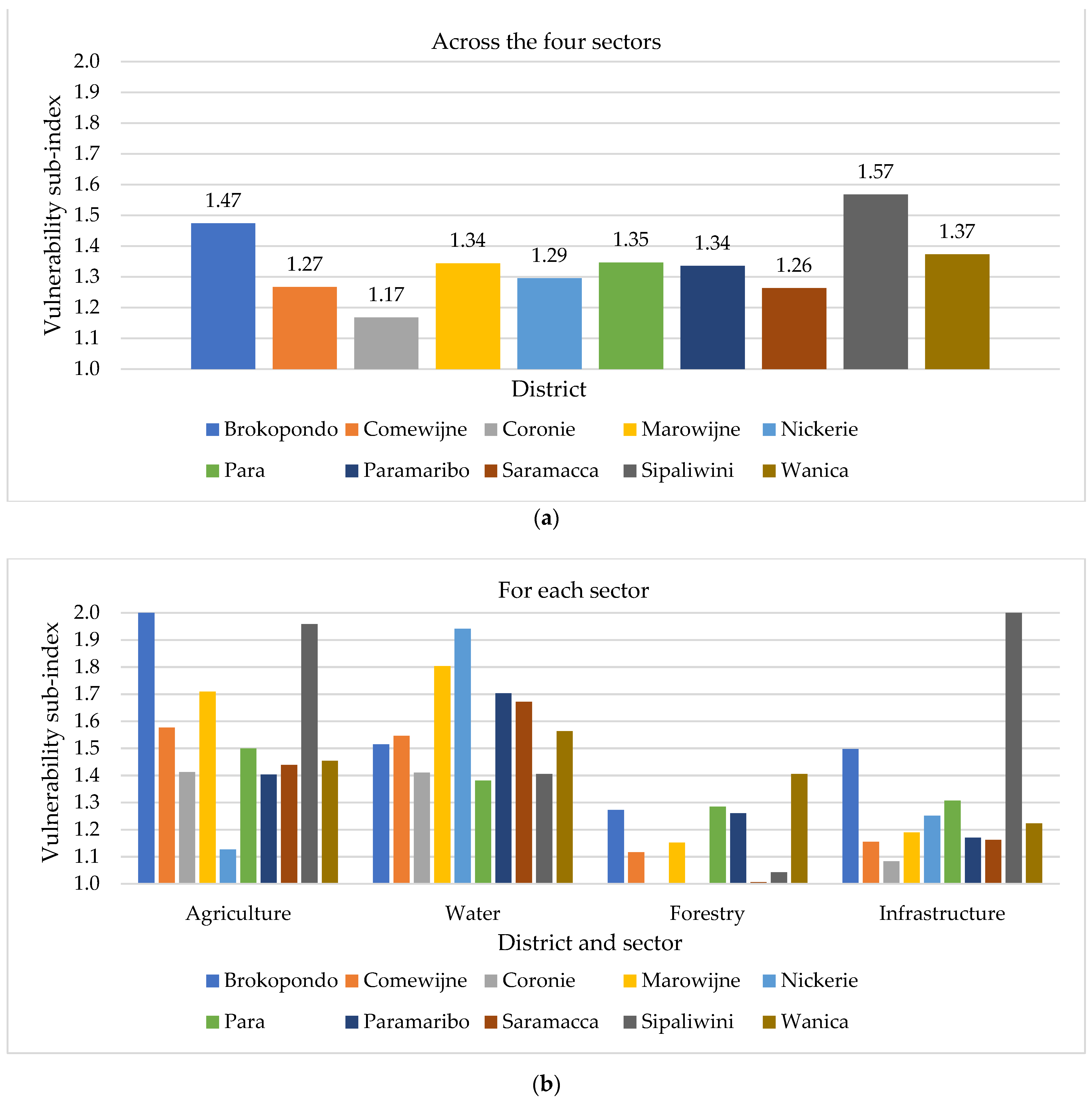
Although Brokopondo is the least exposed district, it is the second most vulnerable district after Sipaliwini (Figure 10a). Brokopondo is the most vulnerable district in agriculture, and the second and third most vulnerable in infrastructure and forestry, respectively (Figure 10b). Sipaliwini is the most vulnerable district in infrastructure and the second most vulnerable district in agriculture. The least vulnerable district is Coronie, with the lowest vulnerability for forestry and infrastructure.

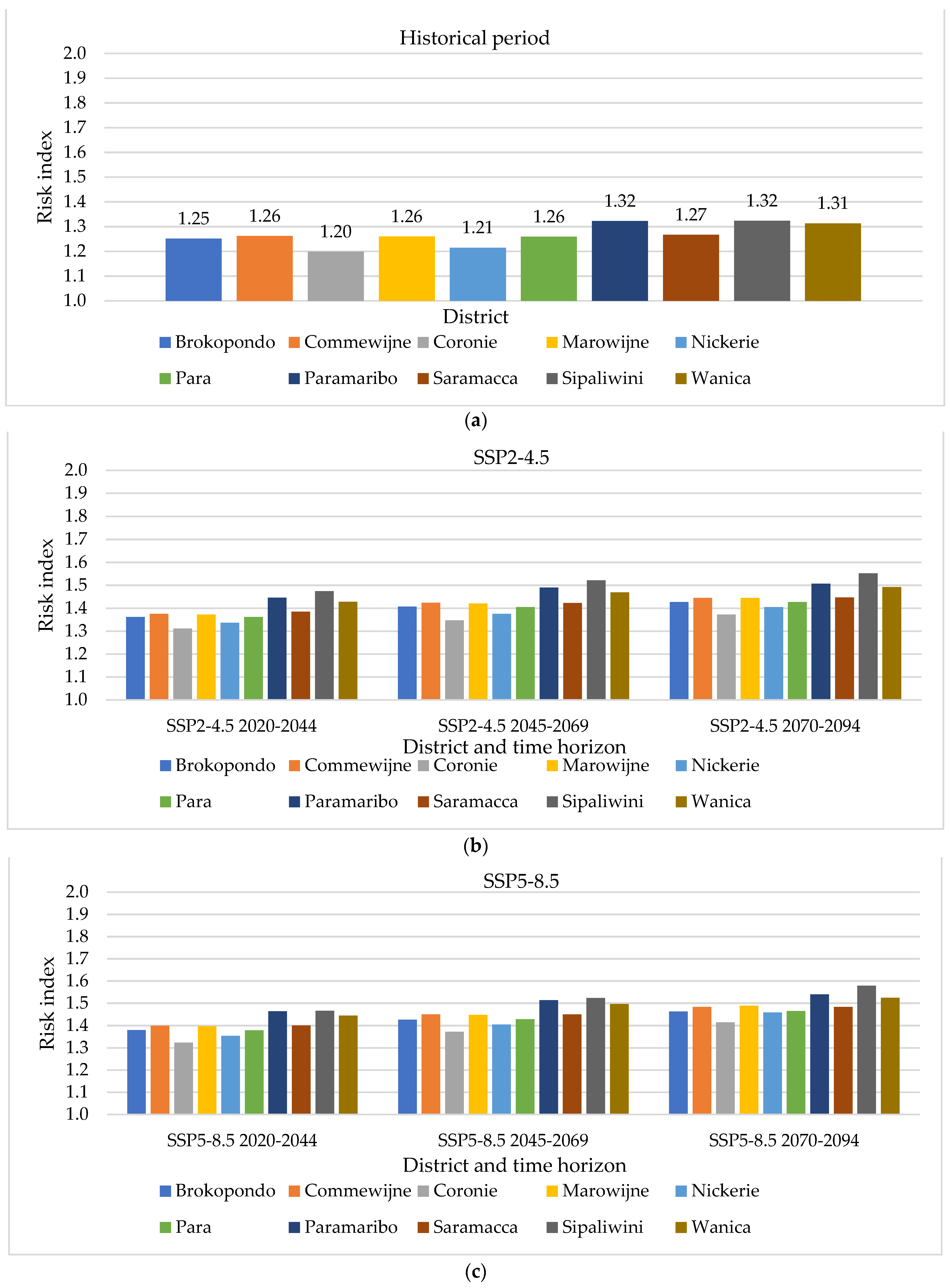
4.4. Risk

As explained in the methodological section, the risk index summarizes the results of the previous sub-indices. At present, Sipaliwini, Paramaribo and Wanica face the highest climate risk (Figure 11a). This is due to the high vulnerability of Sipaliwini’ s infrastructure and agriculture, Paramaribo’s and Wanica’s high hazard sub-index, and its infrastructure exposure. Coronie and Nickerie face the least climate risk. Coronie is the least vulnerable district, with its forestry and infrastructure scoring particularly low, and Nickerie has the lowest hazard sub-index.

Throughout the timeframes of the SSP2-4.5 and SSP5-8.5 scenarios Sipaliwini, Paramaribo and Wanica remain the three districts most at risk in descending order (Figure 11b,c). Coronie and Nickerie remain the districts with the least climate risk in ascending order.

In the SSP2-4.5 and SSP5-8.5 scenarios the difference between the districts most and least at risk increases by 44% and 32%, respectively, between the historical period and the long-term.

5. Discussion

This paper has analysed long-term climate change impacts in Suriname, based on constructing a quality dataset on the historical climate, and the production of robust climate projections for several geographic scales and locations, time horizons and emission scenarios. Climate information was later integrated with a range of highly relevant social and economic indicators. Integrating climate data with current statistical information makes it easier to mainstream climate change into environmental decision-making. It provides a more specific view of the main problems to determine feasible adaptation options and prioritize them.

The goal has been to provide a methodology for SIDS to evaluate climate risks using a quantitative and science-based method, as evaluating climate risks in these countries is a complex task. Limitations in the quantity and quality of current and historical data can be challenging in a context with many institutional challenges [2,3]. Also, research on the field is often more qualitative than quantitative, which is a critical barrier to overcome. Correctly identifying needs and quantifying investments is essential in a context of very limited financial and technical resources [6].

The methodology used in this paper can be replicated in other countries, even in the context of scarce data. However, some limitations of it are worth noting:

-

Uncertainty. Climate projections are uncertain and depend on complex scenarios.

-

Data availability. Climate risk indices can only ever be as good as the indicators and data used to construct them. The limited availability and quality of data particularly at sub-regional levels, constrained the comprehensiveness of the climate risk index, despite assessing a total of 52 indicators.

-

Local irregularities. Indicators show statistical regularities but cannot pinpoint to specific issues or topics at the local level. As a result, the input of local institutions is a crucial element in any analysis.

-

Climate and statistical information can also be complemented by using a monetary approach to quantify the risks. If expected impacts can be quantified, then a cost-benefit analysis can be performed, which has proven effective in other SIDS [37]. Quantifying the costs and benefits reducing climate vulnerability can allow countries to access international climate finance. However, monetary approaches tend to be more expensive and require more data.

Concerning public policy design, this paper confirms that climate change can be a decisive factor for SIDS. Due to that, building local capacities and expertise is essential to ensure the mainstreaming of climate in public and private decision-making. In this regard, before delivering the results of this study, several meetings and consultations with local public institutions and research centers were held. Moreover, three specific capacity training building sessions were conducted on the methods and results of this research.

6. Conclusions

Like most Small Island Developing States, Suriname is highly vulnerable to climate change impacts, due to geographical, climate and socio-economic reasons. Considering the literature on the impact of climate change in the country, it was necessary to conduct a high-resolution study that could model small-scale changes, taking into account the country’s observations. This study allows us to improve the information on the impacts of climate change, which will help provide a stronger scientific and technical basis for public and private sector decision-making in the country.

Climate projections were developed based on three climate models generated in the framework of the CMIP6. Based on these, the temperature is expected to increase throughout the country, for all regions and timeframes, reaching a warming of up to 6 °C in the southern region in the long-term future (2070–2094), particularly during the dry season and under the SSP5-8.5 scenario. Projections point towards a gradual reduction in precipitation, particularly in the southwest and coastal regions and under the SSP-8.5 scenario. The change in its annual distribution is also very relevant, as the dry season is expected to become wetter, and the rainy season is expected to become drier. The mean sea level is also expected to rise. However, different scenarios provide a very different climate forecast of this variable, so further research is necessary. These results are consistent with previous work in northern South America [38,39] and with results being shown globally, including the trend and acceleration of climate change [40] and its effects [41].

Using a risk index, the most impacted regions and sectors have been identified and analyzed using 19 indicators for hazard, 20 for exposure and 13 for vulnerability. Sipaliwini, Paramaribo and Wanica currently face the highest climate risk, whereas Coronie and Nickerie show the lowest scores. When considering the sectoral vulnerability, water and agriculture stand out with high scores in many districts. Forestry shows lower scores, and infrastructure shows varied results, with high scores in Sipaliwini and Paramaribo but relatively low in the others.

In the SSP2-4.5 and SSP5-8.5 scenarios, the results are worse for all districts, particularly under the second scenario. Paramaribo and Wanica remain highly affected, but Sipaliwini becomes one of the districts with the highest score. There is no change in the districts at the top and the bottom of the list.

References

- Avellan, T.; Castonguay, S. A Pathway to Climate Services for SIDS. World Meteorol. Organ. Bull. 2015, 64, 1–10. [Google Scholar]
- Robinson, S.A. Climate change adaptation trends in Small Island Developing States. Mitig. Adapt. Strateg. Glob. Change 2017, 22, 669–691. [Google Scholar] [CrossRef]
- Klöck, C.; Nunn, P.D. Adaptation to Climate Change in Small Island Developing States: A Systematic Literature Review of Academic Research. J. Environ. Dev. 2019, 28, 196–218. [Google Scholar] [CrossRef]
- Nurse, L.A.; McLean, R.F.; Agard, J.; Briguglio, L.P.; Duvat-Magnan, V.; Pelesikoti, N.; Tompkins, E.; Webb, A. Small Islands. In Climate Change 2014—Impacts, Adaptation and Vulnerability: Part B: Regional Aspects; Cambridge University Press: Cambridge, UK, 2015; pp. 1613–1654. [Google Scholar] [CrossRef]
- Saavedra, J.J.; Alleng, G.P. Sustainable Islands: Defining a Sustainable Development Framework Tailored to the Needs of Islands. IDB Tech. Note 2020, 2053, 1–72. [Google Scholar]
- Petzold, J.; Magnan, A.K. Climate change: Thinking small islands beyond Small Island Developing States (SIDS). Clim. Change 2019, 152, 145–165. [Google Scholar] [CrossRef]
- Ministry of Foreign Affairs. National Report in Preparation of the Third International Conference on Small Island Developing States. In Proceedings of the Suriname Report On Sids Conference, Paramaribo, Suriname, 27 July 2013. [Google Scholar]
- Robinson, S.A. Adapting to climate change at the national level in Caribbean Small Island Developing States. Isl. Stud. J. 2018, 13, 79–100. [Google Scholar] [CrossRef]
- Toorman, E.A.; Anthony, E.; Augustinus, P.G.E.F.; Gardel, A.; Gratiot, N.; Homenauth, O.; Huybrechts, N.; Monbaliu, J.; Moseley, K.; Naipal, S. Interaction of Mangroves, Coastal Hydrodynamics, and Morphodynamics along the Coastal Fringes of the Guianas. In Threats to Mangrove Forests: Hazards, Vulnerability, and Management; Springer: Berlin/Heidelberg, Germany, 2018; Volume 25, ISBN 9783319730165. [Google Scholar]
- Pan American Health Organization (PAHO). Health in the Americas, Country Volume Suriname, 2012 ed.; Pan American Health Organization: Washington, DC, USA, 2012. [Google Scholar]
- Nurmohamed, R.; Naipal, S. Development of scenarios for future climate change in Suriname. Acta Nov. 2006, 3, 475–487. [Google Scholar]
- McSweeney, C.; New, M.; Lizcano, G. UNDP Climate Change Country Profiles-Suriname; United Nations Development Programme: New York, NY, USA, 2017. [Google Scholar]
- Almagro, A.; Oliveira, P.T.S.; Nearing, M.A.; Hagemann, S. Projected climate change impacts in rainfall erosivity over Brazil. Sci. Rep. 2017, 7, 8103. [Google Scholar] [CrossRef] [Green Version]
- Peel, M.C.; Finlayson, B.L.; McMahon, T.A. Updated world map of the Köppen-Geiger climate classification. Hydrol. Earth Syst. Sci. 2007, 11, 1633–1644. [Google Scholar] [CrossRef] [Green Version]
- O’Neill, B.C.; Tebaldi, C.; Van Vuuren, D.P.; Eyring, V.; Friedlingstein, P.; Hurtt, G.; Knutti, R.; Kriegler, E.; Lamarque, J.F.; Lowe, J.; et al. The Scenario Model Intercomparison Project (ScenarioMIP) for CMIP6. Geosci. Model Dev. 2016, 9, 3461–3482. [Google Scholar] [CrossRef] [Green Version]
- Nakicenovic, N.; Lempert, R.J.; Janetos, A.C. A Framework for the development of new socio-economic scenarios for climate change research: Introductory essay: A forthcoming special issue of Climatic Change. Clim. Change 2014, 122, 351–361. [Google Scholar] [CrossRef] [Green Version]
- Meinshausen, M.; Nicholls, Z.R.J.; Lewis, J.; Gidden, M.J.; Vogel, E.; Freund, M.; Beyerle, U.; Gessner, C.; Nauels, A.; Bauer, N.; et al. The shared socio-economic pathway (SSP) greenhouse gas concentrations and their extensions to 2500. Geosci. Model Dev. 2020, 13, 3571–3605. [Google Scholar] [CrossRef]
- Amengual, A.; Homar, V.; Romero, R.; Alonso, S.; Ramis, C. A statistical adjustment of regional climate model outputs to local scales: Application to Platja de Palma, Spain. J. Clim. 2012, 25, 939–957. [Google Scholar] [CrossRef] [Green Version]
- Amengual, A.; Homar, V.; Romero, R.; Alonso, S.; Ramis, C. Projections of the climate potential for tourism at local scales: Application to Platja de Palma, Spain. Int. J. Climatol. 2012, 32, 2095–2107. [Google Scholar] [CrossRef] [Green Version]
- Zawadzki, I. Reflectivity-Rain Rate Relationships for Radar Hydrology in Brazil. J. Clim. Appl. Meteorol. Climatol. 1987, 26, 118–132. [Google Scholar]
- Mcinnes, K.L.; Erwin, T.A.; Bathols, J.M. Global Climate Model projected changes in 10 m wind speed and direction due to anthropogenic climate change. Atmos. Sci. Lett. 2011, 12, 325–333. [Google Scholar] [CrossRef]
- D’Amato, G.; Holgate, S.T.; Pawankar, R.; Ledford, D.K.; Cecchi, L.; Al-Ahmad, M.; Al-Enezi, F.; Al-Muhsen, S.; Ansotegui, I.; Baena-Cagnani, C.E.; et al. Meteorological conditions, climate change, new emerging factors, and asthma and related allergic disorders. A statement of the World Allergy Organization. World Allergy Organ. J. 2015, 8, 25. [Google Scholar] [CrossRef] [Green Version]
- Sims, R.E.H. Renewable energy: A response to climate change. Sol. Energy 2004, 76, 9–17. [Google Scholar] [CrossRef]
- Costa, R.L.; Macedo de Mello Baptista, G.; Gomes, H.B.; Daniel dos Santos Silva, F.; Lins da Rocha Júnior, R.; de Araújo Salvador, M.; Herdies, D.L. Analysis of climate extremes indices over northeast Brazil from 1961 to 2014. Weather Clim. Extrem. 2020, 28, 100254. [Google Scholar] [CrossRef]
- Baker, H.S.; Millar, R.J.; Karoly, D.J.; Beyerle, U.; Guillod, B.P.; Mitchell, D.; Shiogama, H.; Sparrow, S.; Woollings, T.; Allen, M.R. Higher CO2 concentrations increase extreme event risk in a 1.5 °C world. Nat. Clim. Change 2018, 8, 604–608. [Google Scholar] [CrossRef] [Green Version]
- Bador, M.; Boé, J.; Terray, L.; Alexander, L.V.; Baker, A.; Bellucci, A.; Haarsma, R.; Koenigk, T.; Moine, M.P.; Lohmann, K.; et al. Impact of Higher Spatial Atmospheric Resolution on Precipitation Extremes Over Land in Global Climate Models. J. Geophys. Res. Atmos. 2020, 125, e2019JD032184. [Google Scholar] [CrossRef]
- Han, W.; Stammer, D.; Thompson, P.; Ezer, T.; Palanisamy, H.; Zhang, X.; Domingues, C.M.; Zhang, L.; Yuan, D. Impacts of Basin-Scale Climate Modes on Coastal Sea Level: A Review. Surv. Geophys. 2019, 40, 1493–1541. [Google Scholar] [CrossRef] [PubMed] [Green Version]
- IPCC. Climate Change, Adaptation, and Vulnerability; Cambridge University Press: London, UK; New York, NY, USA, 2014. [Google Scholar]
- Lissner, T.K.; Holsten, A.; Walther, C.; Kropp, J.P. Towards sectoral and standardised vulnerability assessments: The example of heatwave impacts on human health. Clim. Change 2012, 112, 687–708. [Google Scholar] [CrossRef]
- Saisana, M.; Tarantola, S. State-of-the-Art Report on Current Methodologies and Practices for Composite Indicator Development; Joint Research Centre, European Commission: Ispra, Italy, 2002; EUR 20408 EN. [Google Scholar]
- Nardo, M.; Saisana, M. OECD/JRC Handbook on Constructing Composite Indicators. Putting Theory into Practice; European Commission-Joint Research Centre: Ispra, Italy, 2008. [Google Scholar]
- Boedhram, N. An Agro Climatic Survey of Suriname (Period 1971–1985); Ministry of Public Works Telecommunication and Construction; Meteorological Service of Suriname: Paramaribo, Suriname, 1988; ISBN 9780827028371. [Google Scholar]
- Elsner, J.B.; Kossin, J.P.; Jagger, T.H. The increasing intensity of the strongest tropical cyclones. Nature 2008, 455, 92–95. [Google Scholar] [CrossRef]
- Blennow, K.; Olofsson, E. The probability of wind damage in forestry under a changed wind climate. Clim. Change 2008, 87, 347–360. [Google Scholar] [CrossRef]
- Barreca, A. Climate change, humidity, and mortality in the United States. J. Environ. Econ. Manag. 2012, 63, 19–34. [Google Scholar] [CrossRef] [Green Version]
- Sherwood, S.C.; Ingram, W.; Tsushima, Y.; Satoh, M.; Roberts, M.; Vidale, P.L.; O’Gorman, P.A. Relative humidity changes in a warmer climate. J. Geophys. Res. Atmos. 2010, 115, 1–11. [Google Scholar] [CrossRef] [Green Version]
- Alleng, G. Understanding the Economics of Climate Change Adaptation in Trinidad and Tobago; IDB Monographs, 219; Inter-American Development Bank: Washington, DC, USA, 2014. [Google Scholar]
- Aguilar, E.; Peterson, T.C.; Obando, P.R.; Frutos, R.; Retana, J.A.; Solera, M.; Soley, J.; García, I.G.; Araujo, R.M.; Santos, A.R.; et al. Changes in precipitation and temperature extremes in Central America and northern South America, 1961–2003. J. Geophys. Res. Atmos. 2005, 110, 1–15. [Google Scholar] [CrossRef]
- Wang, B.; Biasutti, M.; Byrne, M.P.; Castro, C.; Chang, C.P.; Cook, K.; Fu, R.; Grimm, A.M.; Ha, K.J.; Hendon, H.; et al. Monsoons climate change assessment. Bull. Am. Meteorol. Soc. 2021, 102, E1–E19. [Google Scholar] [CrossRef]
- IPCC. Climate Change 2021: The Physical Science Basis; Intergovernmental Panel on Climate Change: Geneva, Switzerland, 2021.
- Shukla, P.R.; Skea, J.; Buendia, E.C.; Masson-Delmotte, V.; Pörtner, H.-O.; Roberts, D.C.; Zhai, P.; Slade, R.; Connors, S.; van Diemen, R.; et al. Climate Change and Land: An IPCC Special Report on Climate Change, Desertification, Land Degradation, Sustainable Land Management, Food Security, and Greenhouse Gas Fluxes in Terrestrial Ecosystems; Intergovernmental Panel on Climate Change: Geneva, Switzerland, 2019.
Figure 1.
Geographical location of the weather stations used for calibration. Note: the blue crosses indicate rainfall stations, and the red asterisks indicate thermo-pluviometric stations. In addition, this map shows the limited coverage of the network, especially in terms of thermo-pluviometric stations.
Figure 2.
Example of an impact chain developed for the agriculture sector, including hazards (blue), intermediate impacts (grey), exposed elements (yellow), vulnerability factors (green), and risk (red). Source: own elaboration.
Figure 3.
Geographical position of the study area, Suriname.
Figure 4.
Reference period spatial distribution of: (a) mean temperature; (b) mean annual accumulated precipitation; (c) mean max wind values; (d) mean relative humidity.
Figure 5.
Comparison of mean temperature in both scenarios and the effects on the TX09p indices in the long-term future. (a) Spatial distribution of mean temperature under the SSP2-4.5 scenario in the short-term future. (b) Spatial distribution of mean temperature under the SSP5-8.5 scenario in the short-term future. (c) Spatial distribution of mean temperature under the SSP2-4.5 scenario in the long-term future. (d) Spatial distribution of mean temperature under the SSP5-8.5 scenario in the long-term future. (e) Spatial distribution of frequency of hot days under the SSP2-4.5 scenario in the long-term future. (f) Spatial distribution of frequency of hot days under the SSP5-8.5 scenario in the long-term future.
Figure 6.
Results of spatial and seasonal precipitation projections: (a) Spatial distribution for the anomaly of projected mean accumulated rainfall for the long-term future under SSP2-4.5 scenario; (b) Spatial distribution for the anomaly of projected mean accumulated rainfall for long-term future under SSP5-8.5 scenario; (c) Projected accumulations for the SSP2-4.5 scenario for each of the Surinamese stations; (d) Projected accumulations for the SSP5-8.5 scenario for each station.
Figure 7.
Mean sea level anomaly off the coast of Suriname and associated uncertainties.
Figure 8.
Results of the hazard sub-index across the ten districts for (a) the historical period, (b) the SSP2-4.5 scenario and three future time horizons and (c) the SSP5-8.5 scenario and three future time horizons.
Figure 9.
Results of the exposure sub-index for the ten districts (a) across the four sectors and (b) for each.
Figure 10.
Results of the vulnerability sub-index for the ten districts (a) across the four sectors and (b) for each one of them.
Figure 11.
Results of the risk index for the ten districts for (a) the historical period, (b) the SSP2-4.5 scenario and three future time horizons and (c) the SSP5-8.5 scenario and three future time horizons.