
The Challenge of Deploying Failure Modes and Effects Analysis in Complex System Applications—Quantification and Analysis


Abstract
:1. Introduction
- Functional Failure Modes and Effects Analysis (Functional FMEA) to evaluate those failures associated with functional requirements of products and systems;
- Design Failure Modes and Effects Analysis (Design FMEA) to analyse those failures associated with design elements;
- Process Failure Modes and Effects Analysis (Process FMEA) to assess the potential failures encountered in manufacturing and assembly processes.
2. Materials and Methods
2.1. Data Preparation
2.1.1. Construction of the Dependent Variable
2.1.2. Construction of the Independent Variables
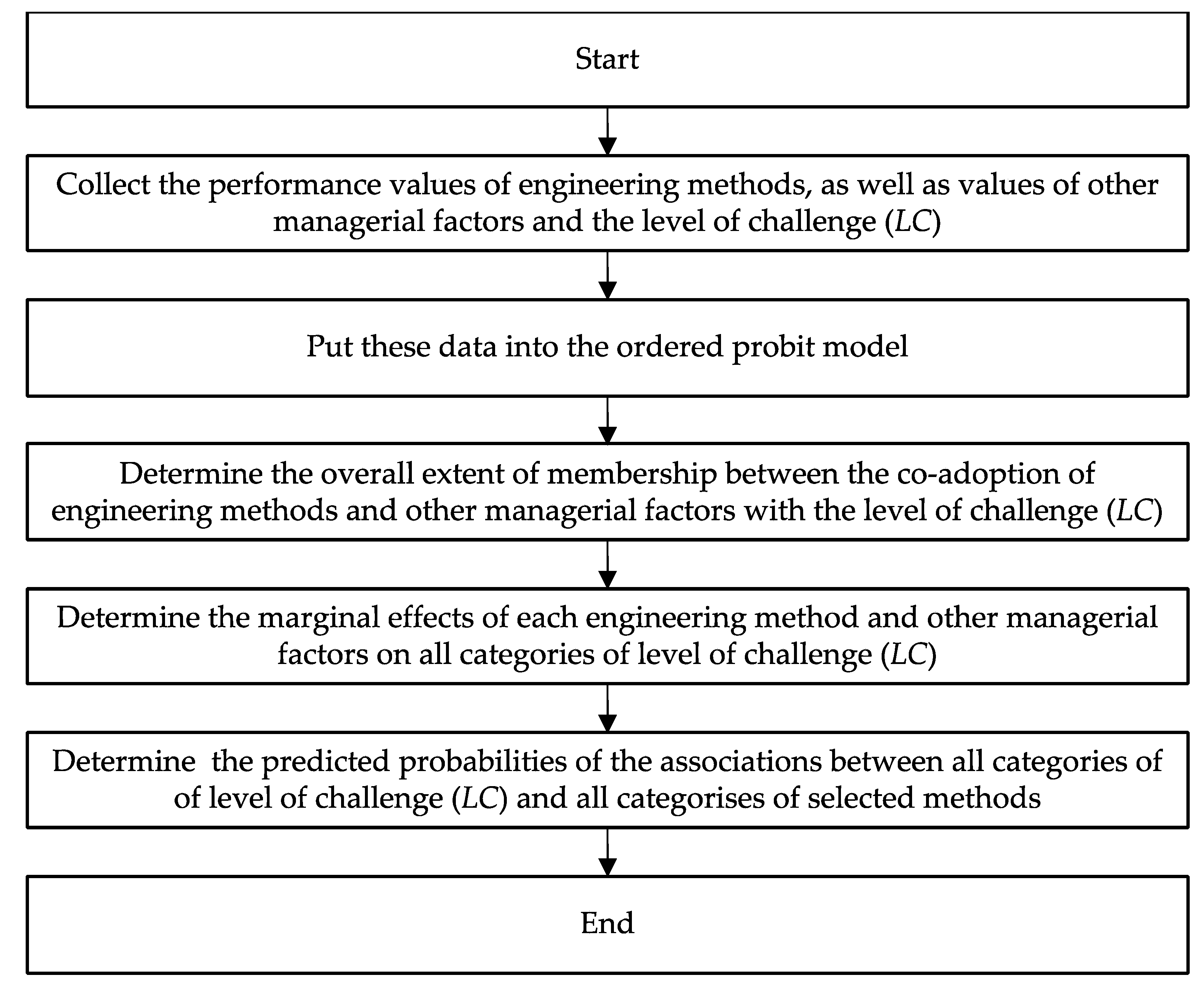
2.2. Model Specification for Analysis
3. Results
3.1. Descriptive Statistics
3.2. Model Results
4. Discussion
5. Conclusions
Author Contributions
Funding
Institutional Review Board Statement
Informed Consent Statement
Data Availability Statement
Acknowledgments
Conflicts of Interest
Appendix A

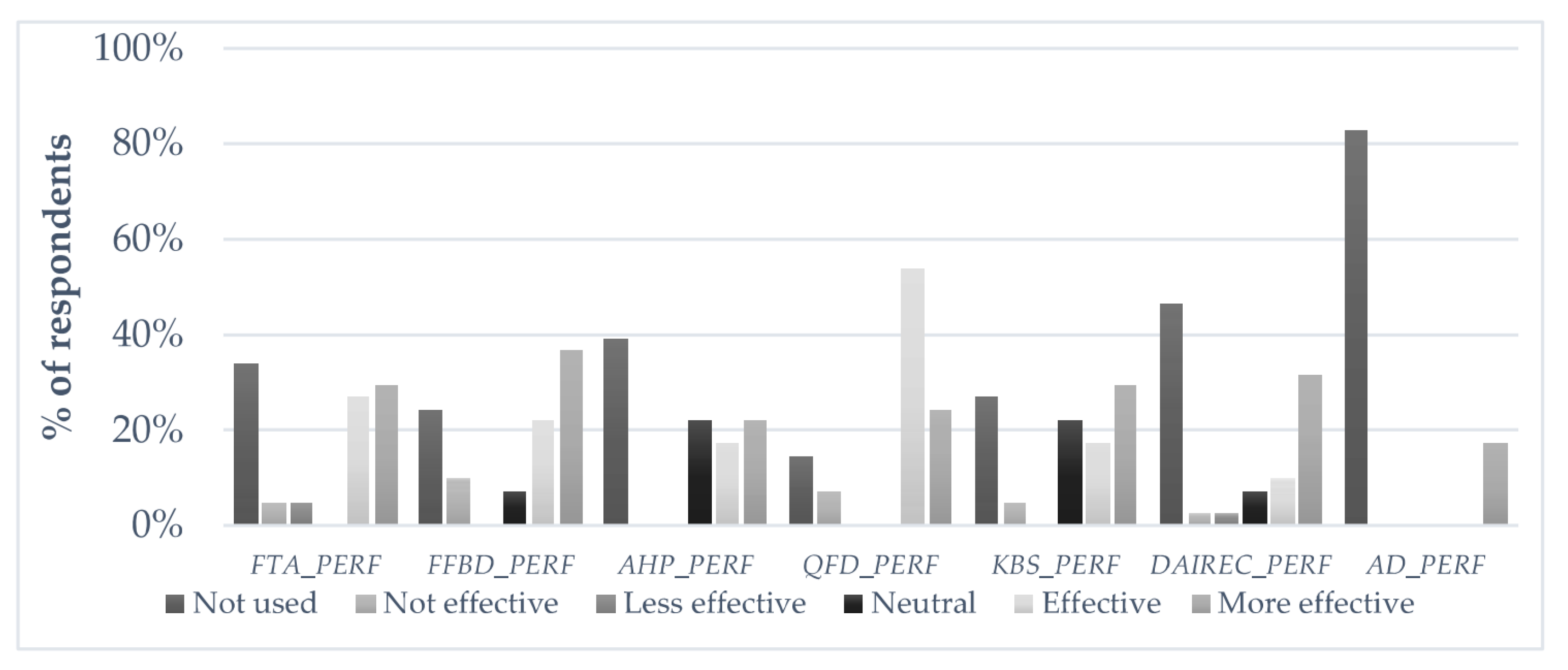
| Variable Name | Symbol | Description | Information Type | Data Source and Remarks |
|---|---|---|---|---|
| Fault Tree Analysis | FTA_PERF | Performance value coded from Likert-scale | Ordered discrete | Questionnaire |
| Functional Flow Boundary Diagram | FFBD_PERF | |||
| Analytical Hierarchical Process | AHP_PERF | |||
| Quality Function Deployment | QFD_PERF | |||
| Knowledge-Based System | KBS_PERF | |||
| Define, Analysis, Improve, Recommend, Evaluate and Control | DAIREC_PERF | |||
| Axiomatic Design | AD_PERF | |||
| Experience Level | EXP | Coded as follows: EXP = 0, if the number of experiences = <9 EXP = 1, if the number of experiences > 9 and = <15 EXP = 2, if the number of experiences > 15 and = <23 EXP = 3, if the number of experiences > 23 and = <30 EXP = 4, if the number of experiences > 30 | Continuous | LinkedIn profiles and face-to-face questions |
| Organisational size | SIZE | Coded as follows: SIZE = 0, if the number of employees <=20,000 SIZE = 1, if the number of employees > 20,000 and =<50,000 SIZE = 2, if the number of employees > 50,000 and =<100,000 SIZE = 3, if the number of employees > 100,000 and =<250,000 SIZE = 4, if the number of employees > 250,000 | Annual reports of businesses | |
| Industry membership | MEM | Industry membership values coded from participants fields of work | Binary | LinkedIn profiles and face-to-face questions |
| Level of challenge to deploy FMEA (dependent variable) | LC | Score variable consisting of the following challenges: Excessive use of resources Applicability Capture interaction failures between system, sub-system and components levels The knowledge gap between design and manufacturing phases Inability to trace risks | Ordered discrete | Questionnaire, composed from multiple questions |
| Variable Name | Symbol | Description | Information Type | Data Source and Remarks |
|---|---|---|---|---|
| Fault Tree Analysis | FTA_m | Taking FTA_m as illustrative to represent all listed variables, the coding as follows: FTA_m = 0, if FTA_PERF = 0 FTA_m = 1, if FTA_PERF = 1 & 2 FTA_m = 2, if FTA_PERF = 3 & 4 FTA_m = 3, if FTA_PERF = 5 | Ordered discrete | Original formed Likert scales |
| Functional Flow Boundary Diagram | FFBD_m | |||
| Analytical Hierarchical Process | AHP_m | |||
| Quality Function Deployment | QFD_m | |||
| Knowledge-Based System | KBS_m | |||
| Define, Analysis, Improve, Recommend, Evaluate and Control | DAIREC_m | |||
| Axiomatic Design | AD_m | |||
| Experience Level | EXP_m | Recoded as follows: EXP_m = 0, if EXP = 0 & 1 EXP_m = 1, if EXP = 2 EXP_m = 2, if EXP = 3 EXP_m = 3, if EXP = 4 | Continuous | |
| Organisational size | SIZE_m | Recoded as follows: SIZE_m = 0, if SIZE = 0 &1 SIZE_m = 1, if SIZE = 2 SIZE_m = 2, if SIZE = 3 SIZE_m = 3, if SIZE = 4 | ||
| Industry membership (Kept same) | MEM | Industry membership values coded from participants fields of work | Binary | LinkedIn profiles and face-to-face questions |
| Level of challenge to deploy FMEA (dependent variable) | LC_m | Recoded as follows: LC_m = 0, if LC = 0 & 1 LC_m = 1, if LC = 2 LC_m = 2, if LC = 3 LC_m = 3, if LC = 4 & 5 | Ordered discrete | Questionnaire, composed from multiple questions |
| Observation | LC | FTA_ PERF | FFBD_PERF | AHP_PERF | QFD_PERF | KBS_ PERF | DAIREC_PERF | AD_ PERF | EXP | SIZE | MEM |
|---|---|---|---|---|---|---|---|---|---|---|---|
| Discrete | Discrete | Discrete | Discrete | Discrete | Discrete | Discrete | Discrete | Continuous | Continuous | Binary | |
| 1 | 4 | 0 | 5 | 0 | 5 | 0 | 0 | 0 | 25 | 43,224 | 1 |
| 2 | 2 | 5 | 0 | 3 | 4 | 1 | 1 | 0 | 20 | 9500 | 0 |
| 3 | 4 | 0 | 0 | 3 | 5 | 0 | 0 | 0 | 14 | 30,000 | 1 |
| 4 | 3 | 4 | 5 | 5 | 4 | 0 | 5 | 0 | 10 | 237,000 | 1 |
| 5 | 4 | 0 | 5 | 0 | 5 | 4 | 0 | 0 | 16 | 26,004 | 1 |
| 6 | 4 | 5 | 3 | 0 | 5 | 0 | 4 | 0 | 42 | 9989 | 1 |
| 7 | 4 | 0 | 5 | 5 | 4 | 5 | 5 | 0 | 8 | 153,000 | 0 |
| 8 | 4 | 4 | 0 | 0 | 4 | 0 | 0 | 0 | 10 | 137,250 | 1 |
| 9 | 3 | 5 | 1 | 5 | 4 | 5 | 0 | 0 | 21 | 3205 | 0 |
| 10 | 5 | 0 | 1 | 5 | 4 | 5 | 0 | 0 | 11 | 61,117 | 0 |
| 11 | 3 | 0 | 0 | 0 | 4 | 5 | 5 | 0 | 26 | 37,543 | 1 |
| 12 | 4 | 4 | 0 | 3 | 4 | 3 | 0 | 0 | 11 | 237,000 | 1 |
| 13 | 5 | 0 | 0 | 4 | 4 | 4 | 0 | 0 | 43 | 54,500 | 1 |
| 14 | 5 | 0 | 0 | 0 | 4 | 0 | 0 | 0 | 20 | 3205 | 0 |
| 15 | 2 | 5 | 5 | 3 | 4 | 5 | 5 | 0 | 19 | 3205 | 0 |
| 16 | 3 | 4 | 3 | 0 | 0 | 3 | 0 | 0 | 7 | 105,000 | 0 |
| 17 | 2 | 4 | 5 | 5 | 1 | 3 | 5 | 0 | 29 | 61,117 | 0 |
| 18 | 3 | 1 | 4 | 4 | 4 | 5 | 5 | 0 | 21 | 85,000 | 0 |
| 19 | 4 | 5 | 4 | 3 | 5 | 5 | 0 | 0 | 9 | 9500 | 0 |
| 20 | 2 | 4 | 5 | 4 | 4 | 3 | 5 | 0 | 8 | 3205 | 0 |
| 21 | 1 | 5 | 5 | 5 | 1 | 5 | 0 | 5 | 13 | 43,224 | 1 |
| 22 | 3 | 4 | 0 | 0 | 4 | 3 | 0 | 0 | 8 | 173,000 | 1 |
| 23 | 3 | 4 | 4 | 0 | 5 | 0 | 0 | 0 | 13 | 54,500 | 0 |
| 24 | 4 | 0 | 5 | 0 | 5 | 5 | 5 | 0 | 14 | 48,000 | 0 |
| 25 | 3 | 0 | 5 | 3 | 4 | 4 | 0 | 0 | 26 | 237,000 | 1 |
| 26 | 2 | 4 | 3 | 3 | 4 | 4 | 4 | 0 | 28 | 237,000 | 1 |
| 27 | 2 | 4 | 4 | 3 | 4 | 3 | 4 | 0 | 15 | 237,000 | 1 |
| 28 | 1 | 5 | 4 | 4 | 0 | 5 | 4 | 5 | 11 | 37,543 | 1 |
| 29 | 1 | 5 | 1 | 5 | 0 | 0 | 5 | 0 | 8 | 61,117 | 0 |
| 30 | 3 | 0 | 0 | 0 | 4 | 3 | 0 | 0 | 15 | 9500 | 1 |
| 31 | 2 | 5 | 4 | 4 | 4 | 5 | 3 | 0 | 15 | 43,224 | 1 |
| 32 | 1 | 5 | 5 | 0 | 0 | 5 | 0 | 5 | 20 | 173,000 | 1 |
| 33 | 1 | 4 | 4 | 3 | 1 | 4 | 3 | 5 | 18 | 153,000 | 0 |
| 34 | 2 | 2 | 5 | 0 | 4 | 3 | 5 | 0 | 5 | 3205 | 0 |
| 35 | 2 | 0 | 5 | 4 | 5 | 3 | 2 | 0 | 29 | 211,915 | 1 |
| 36 | 1 | 5 | 5 | 5 | 0 | 1 | 5 | 5 | 17 | 133671 | 0 |
| 37 | 3 | 1 | 0 | 0 | 4 | 0 | 0 | 5 | 21 | 237,000 | 1 |
| 38 | 2 | 2 | 5 | 0 | 4 | 0 | 5 | 0 | 20 | 655,700 | 1 |
| 39 | 4 | 0 | 4 | 5 | 5 | 0 | 0 | 0 | 27 | 153,000 | 0 |
| 40 | 3 | 0 | 4 | 0 | 5 | 4 | 3 | 0 | 8 | 61,117 | 0 |
| 41 | 0 | 5 | 1 | 4 | 0 | 4 | 5 | 5 | 6 | 237,000 | 1 |
- To optimise the dependent variable: LC1.1. Gen LC_m = 0 if LC = 0|LC = 11.2. Replace LC_m = 1 if LC = 21.3. Replace LC_m = 2 if LC = 31.4. Replace LC_m =3 if LC = 4|LC = 5
- To optimise the independent variables2.1. Gen FTA_m = 0 if FTA_PERF = 02.2. Replace FTA_m = 1 if FTA_PERF = 1|FTA_PERF = 22.3. Replace FTA_m = 2 if FTA_PERF = 3|FTA_PERF = 42.4. Replace FTA_m = 3 if FTA_PERF = 52.5. Gen FFBD_m = 0 if FFBD_PERF = 02.6. Replace FFBD_m = 1 if FFBD_PERF = 1|FFBD_PERF = 22.7. Replace FFBD_m = 2 if FFBD_PERF = 3|FFBD_PERF = 42.8. Replace FFBD_m = 3 FFBD_PERF = 52.9. Gen AHP_m = 0 if AHP_PERF = 02.10. Replace AHP_m = 1 if AHP_PERF = 1|AHP_PERF = 22.11. Replace AHP_m = 2 if AHP_PERF = 3|AHP_PERF = 42.12. Replace AHP_m = 3 if AHP_PERF = 52.13. Gen QFD_m = 0 if QFD_PERF == 02.14. Replace QFD_m = 1 if QFD_PERF = 1|QFD_PERF = 22.15. Replace QFD_m = 2 if QFD_PERF = 3|QFD_PERF = 42.16. Replace QFD_m = 3 if QFD_PERF = 52.17. Gen KBS_m = 0 if KBS_PERF = 02.18. Replace KBS_m = 1 if KBS_PERF = 1|KBS_PERF = 22.19. Replace KBS_m = 2 if KBS_PERF = 3|KBS_PERF = 42.20. Replace KBS_m = 3 if KBS_PERF = 52.21. Gen DAIREC_m = 0 if DAIREC_PERF = 02.22. Replace DAIREC_m = 1 if DAIREC_PERF = 1|DAIREC_PERF = 22.23. Replace DAIREC_m = 2 if DAIREC_PERF = 3|DAIREC_PERF = 42.24. Replace DAIREC_m = 3 if DAIREC_PERF = 52.25. Gen AD_m = 0 if AD_PERF = 02.26. Replace AD_m = 1 if AD_PERF = 1|AD_PERF = 22.27. Replace AD_m = 2 if AD_PERF = 3|AD_PERF = 42.28. Replace AD_m = 3 if AD_PERF = 52.29. Gen EXP_m = 0 if EXP = 0|EXP = 12.30. Replace EXP_m = 1 if EXP = 22.31. Replace EXP_m = 2 if EXP = 32.32. Replace EXP_m = 3 if EXP = 42.33. Gen SIZE_m = 0 if SIZE = 0|SIZE = 12.34. Replace SIZE_m = 1 if SIZE = 22.35. Replace SIZE_m = 2 if SIZE = 32.36. Replace SIZE_m = 3 if SIZE = 4
- To run the ordered probit model3.1. Global ylist LC_m3.2. Global xlist FTA_m FFBD_m AHP_m QFD_m KBS_m DAIREC_m AD_m EXP_m SIZE_m MEM3.3. Describe $ylist $xlist3.4. Summarise $ylist $xlist3.5. Tabulate $ylist3.6. Oprobit $ylist $xlist, level (90)
- To obtain the marginal effects at means4.1. Mfx, predict (outcome (0))4.2. Mfx, predict (outcome (1))4.3. Mfx, predict (outcome (2))4.4. Mfx, predict (outcome (3))
- To obtain the predicted probabilities at means5.1. Predict p1, pr outcome (0)5.2. Predict p2, pr outcome (1)5.3. Predict p3, pr outcome (2)5.4. Predict p4, pr outcome (3)5.5. Summarise p1 p2 p3 p45.6. Tabstat p1 p2 p3 p4, by (FTA_m)5.7. Tabstat p1 p2 p3 p4, by (AD_m)
References
- Carlson, C. Effective FMEAs: Achieving Safe, Reliable, and Economical Products and Processes Using Failure Mode and Effects Analysis; John Wiley & Sons: Hoboken, NJ, USA, 2012; Volume 1. [Google Scholar]
- Stamatis, D.H. Failure Mode and Effect Analysis: FMEA from Theory to Execution; ASQC Quality Press: Milwaukee, WI, USA, 2003. [Google Scholar]
- Chan, S.; Ip, W.; Zhang, W. Integrating failure analysis and risk analysis with quality assurance in the design phase of medical product development. Int. J. Prod. Res. 2012, 50, 2190–2203. [Google Scholar] [CrossRef]
- Hassan, A.; Siadat, A.; Dantan, J.Y.; Martin, P. Conceptual process planning–an improvement approach using QFD, FMEA, and ABC methods. Robot. Comput. Integr. Manuf. 2010, 26, 392–401. [Google Scholar] [CrossRef]
- Tague, N. The Quality Toolbox, 2nd ed.; ASQ Quality Press: Milwaukee, WI, USA, 2004; pp. 236–240. [Google Scholar]
- Peeters, J.; Basten, R.; Tinga, T. Improving failure analysis efficiency by combining FTA and FMEA in a recursive manner. Reliab. Eng. Syst. Saf. 2018, 172, 36–44. [Google Scholar] [CrossRef] [Green Version]
- Spreafico, C.; Russo, D.; Rizzi, C. A state-of-the-art review of FMEA/FMECA including patents. Comput. Sci. Rev. 2017, 25, 19–28. [Google Scholar] [CrossRef]
- Emovon, I.; Norman, R.A.; Alan, J.M.; Pazouki, K. An integrated multicriteria decision making methodology using compromise solution methods for prioritising risk of marine machinery systems. Ocean Eng. 2015, 105, 92–103. [Google Scholar] [CrossRef]
- Onofrio, R.; Piccagli, F.; Segato, F. Failure Mode, Effects and Criticality Analysis (FMECA) for Medical Devices: Does Stand-ardisation Foster Improvements in the Practice? Procedia Manuf. 2015, 3, 43–50. [Google Scholar] [CrossRef] [Green Version]
- Henshall, E.; Campean, I.F.; Rutter, B. A Systems Approach to the Development and Use of FMEA in Complex Automotive Applications. SAE Int. J. Mater. Manuf. 2014, 7, 280–290. [Google Scholar] [CrossRef]
- Vinodh, S.; Santhosh, D. Application of FMEA to an automotive leaf spring manufacturing organisation. TQM J. 2012, 24, 260–274. [Google Scholar] [CrossRef]
- Ebrahimipour, V.; Rezaie, K.; Shokravi, S. An ontology approach to support FMEA studies. Expert Syst. Appl. 2010, 37, 671–677. [Google Scholar] [CrossRef]
- Soufhwee, A.; Hambali, A.; Rahman, M.; Hanizam, H. Development of an Integrated FMEA (i-FMEA) Using DAIREC Methodology for Automotive Manufacturing Company. Appl. Mech. Mater. 2013, 315, 176–180. [Google Scholar] [CrossRef]
- Xiao, N.; Huang, H.-Z.; Li, Y.; He, L.; Jin, T. Multiple failure modes analysis and weighted risk priority number evaluation in FMEA. Eng. Fail. Anal. 2011, 18, 1162–1170. [Google Scholar] [CrossRef]
- Teng, S.G.; Ho, S.M.; Shumar, D.; Liu, P.C. Implementing FMEA in a collaborative supply chain environment. Int. J. Qual. Reliab. Manag 2006, 23, 179–196. [Google Scholar] [CrossRef]
- Kmenta, S.; Ishii, K. Scenario-Based Failure Modes and Effects Analysis Using Expected Cost. J. Mech. Des. 2004, 126, 1027–1035. [Google Scholar] [CrossRef]
- Yu, S.; Liu, J.; Yang, Q.; Pan, M. A comparison of FMEA, AFMEA and FTA. In Proceedings of the the 9th International Conference on Reliability, Maintainability and Safety, Guiyang, China, 12–15 June 2011; pp. 954–960. [Google Scholar]
- Banghart, M.; Bian, L.; Babski-Reeves, K. Human Induced Variability during Failure Mode Effects Analysis (FMEA). In Proceedings of the Reliability and Maintainability Symposium, Tucson, AZ, USA, 25–28 January 2016; pp. 1–7. [Google Scholar]
- Bluvband, Z.; Grabov, P. Failure analysis of FMEA. In Proceedings of the 2009 Annual Reliability and Maintainability Symposium, Fort Worth, TX, USA, 26–29 January 2009; pp. 344–347. [Google Scholar]
- Arcidiacono, G.; Campatelli, G. Reliability Improvement of a Diesel Engine Using the FMETA Approach. Qual. Reliab. Eng. Int. 2004, 20, 143–154. [Google Scholar] [CrossRef]
- Suh, N.P. Axiomatic Design: Advances and Applications; Oxford University Press: Oxford, UK, 2001. [Google Scholar]
- Korayem, M.; Iravani, A. Improvement of 3P and 6R mechanical robots reliability and quality applying FMEA and QFD approaches. Robot. Comput. Manuf. 2008, 24, 472–487. [Google Scholar] [CrossRef]
- White, T.; Stoller, S.L.; Greene, W.D.; Christenson, R.L.; Bowen, B.C. Development of the Functional Flow Block Diagram for the J-2X Rocket Engine System. In Proceedings of the JANNAF Interagency Propulsion Conference, Denver, CA, USA, 14 May 2007. [Google Scholar]
- Sharma, R.K.; Kumar, D.; Kumar, P. Systematic failure mode effect analysis (FMEA) using fuzzy linguistic modelling. Int. J. Qual. Reliab. Manag. 2005, 22, 986–1004. [Google Scholar] [CrossRef]
- Filho, J.C.B.; Piechnicki, F.; Loures, E.D.F.R.; Santos, E.A.P. Process-aware FMEA framework for failure analysis in maintenance. J. Manuf. Technol. Manag. 2017, 28, 822–848. [Google Scholar] [CrossRef]
- Tang, X.; Wang, M.; Wang, S. A systematic methodology for quality control in the product development process. Int. J. Prod. Res. 2007, 45, 1561–1576. [Google Scholar] [CrossRef]
- Bayazit, O. Use of AHP in decision-making for flexible manufacturing systems. J. Manuf. Technol. Manag. 2005, 16, 808–819. [Google Scholar] [CrossRef] [Green Version]
- Gu, Y.K.; Cheng, Z.X.; Qiu, G.Q. An improved FMEA analysis method based on QFD and TOPSIS theory. Int. J. Interact. Des. Manuf. 2019, 13, 617–626. [Google Scholar] [CrossRef]
- Hassan, A.; Siadat, A.; Dantan, J.Y.; Martin, P. Interoperability of QFD, FMEA, and KCs methods in the product development process. In Proceedings of the 2009 IEEE International Conference on Industrial Engineering and Engineering Management, Hong Kong, China, 8–11 December 2009; pp. 403–407. [Google Scholar]
- Augustine, M.; Yadav, O.P.; Jain, R.; Rathore, A. Cognitive map-based system modeling for identifying interaction failure modes. Res. Eng. Des. 2011, 23, 105–124. [Google Scholar] [CrossRef]
- Renu, R.; Visotsky, D.; Knackstedt, S.; Mocko, G.; Summers, J.D.; Schulte, J. A Knowledge Based FMEA to Support Identification and Management of Vehicle Flexible Component Issues. Procedia CIRP 2016, 44, 157–162. [Google Scholar] [CrossRef] [Green Version]
- Alruqi, M.; Baumers, M.; Branson, D.; Farndon, R. A Structured Approach for Synchronising the Applications of Failure Mode and Effects Analysis. Manag. Syst. Prod. Eng. 2021, 29, 165–177. [Google Scholar] [CrossRef]
- Etikan, I.; Musa, S.A.; Alkassim, R.S. Comparison of Convenience Sampling and Purposive Sampling. Am. J. Theor. Appl. Stat. 2016, 5, 1–4. [Google Scholar] [CrossRef] [Green Version]
- Baumers, M.; Tuck, C.; Hague, R. Realised levels of geometric complexity in additive manufacturing. Int. J. Prod. Dev. 2011, 13, 222. [Google Scholar] [CrossRef]
- McKelvey, R.D.; Zavoina, W. A statistical model for the analysis of ordinal level dependent variables. J. Math. Sociol. 1975, 4, 103–120. [Google Scholar] [CrossRef]
- Chan, G.; Miller, P.; Tcha, M. Happiness in University Education. Int. Rev. Econ. Educ. 2005, 4, 20–45. [Google Scholar] [CrossRef]
- Aldrich, J.; Nelson, F.; Alder, E.S. MLinear Probability, Logit, and Probit Models; Sage Publications: Newbury Park, CA, USA, 1984. [Google Scholar]
- Cameron, T. A new paradigm for valuing non-market goods using referendum data: Maximum likelihood estimation by cen-sored logistic regression. J. Environ. Econ. Manage. 1988, 15, 355–379. [Google Scholar] [CrossRef]
- Jackman, S. Models for ordered outcomes. Pol. Sci. 2000, 150C/350C, 1–20. [Google Scholar]
- Payton, M.E.; Greenstone, M.H.; Schenker, N. Overlapping confidence intervals or standard error intervals: What do they mean in terms of statistical significance? J. Insect Sci. 2003, 3, 34. [Google Scholar] [CrossRef]
- Schenker, N.; Gentleman, J.F. On Judging the Significance of Differences by Examining the Overlap between Confidence Intervals. Am. Stat. 2001, 55, 182–186. [Google Scholar] [CrossRef]
- Coelho, A.G.; Mourão, A.; Pereira, Z.L. Improving the use of QFD with Axiomatic Design. Concurr. Eng. 2005, 13, 233–239. [Google Scholar] [CrossRef]
- Fargnoli, M.; Sakao, T. Uncovering differences and similarities among quality function deployment-based methods in Design for X: Benchmarking in different domains. Qual. Eng. 2016, 29, 690–712. [Google Scholar] [CrossRef]
- Shaker, F.; Shahin, A.; Jahanyan, S. Developing a two-phase QFD for improving FMEA: An integrative approach. Int. J. Qual. Reliab. Manag. 2019, 36, 1454–1474. [Google Scholar] [CrossRef]
- Futia, G.; Vetrò, A. On the Integration of Knowledge Graphs into Deep Learning Models for a More Comprehensible AI—Three Challenges for Future Research. Information 2020, 11, 122. [Google Scholar] [CrossRef] [Green Version]
- Peres, R.S.; Rocha, A.D.; Leitao, P.; Barata, J. IDARTS—Towards intelligent data analysis and real-time supervision for industry 4. Comput. Ind. 2018, 101, 138–146. [Google Scholar] [CrossRef] [Green Version]
- Santos, M.Y.; e Sá, J.O.; Costa, C.; Galvão, J.; Andrade, C.; Martinho, B.; Lima, F.V.; Costa, E. A Big Data Analytics Architecture for Industry 4.0. In World Conference on Information Systems and Technologies; Springer: Cham, Switzerland, 2017; pp. 175–184. [Google Scholar]
- Lo, H.-W.; Shiue, W.; Liou, J.J.H.; Tzeng, G.-H. A hybrid MCDM-based FMEA model for identification of critical failure modes in manufacturing. Soft Computing. 2020, 24, 15733–15745. [Google Scholar] [CrossRef]
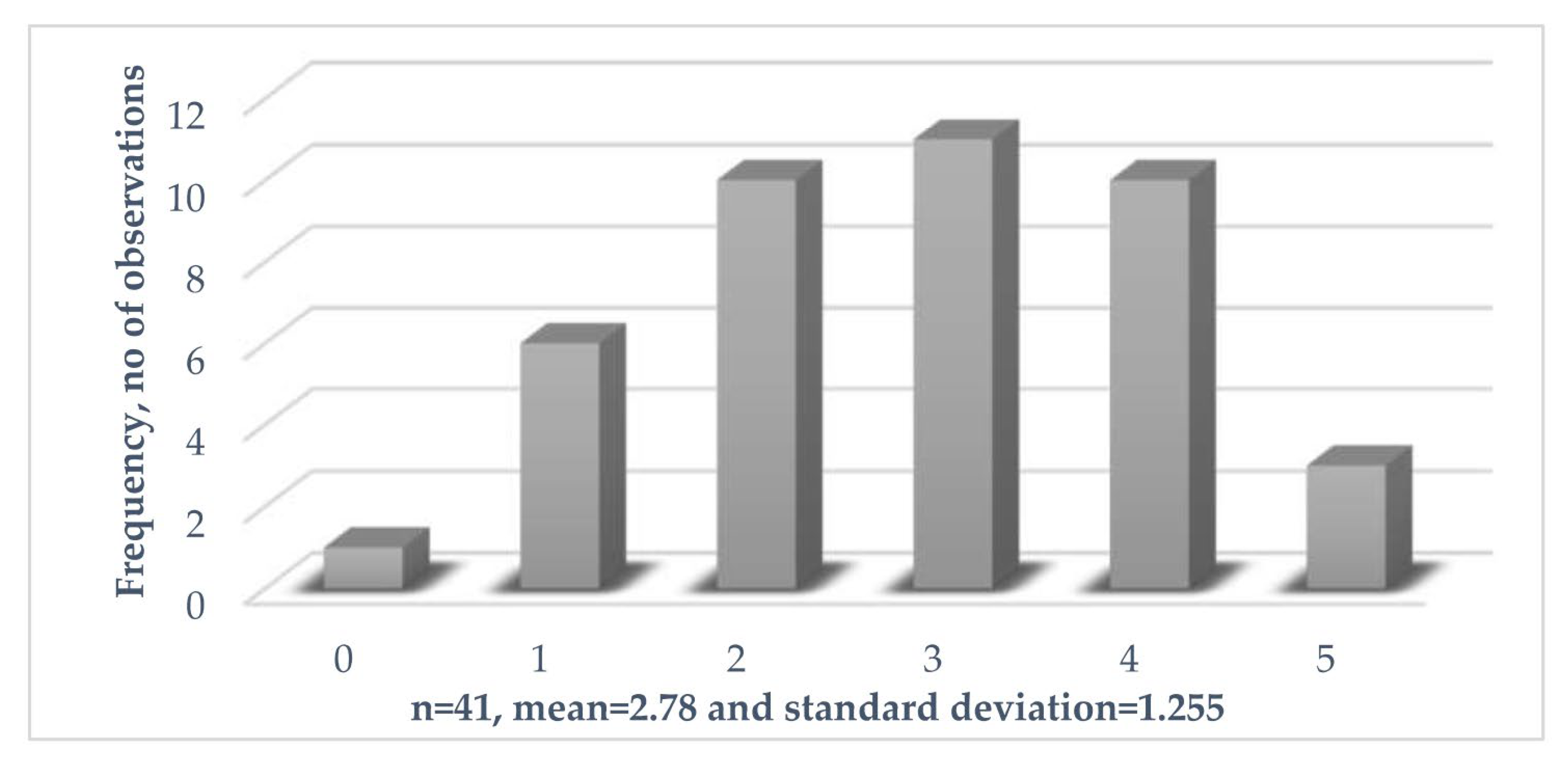
| Mean | Standard Deviation | Minimum | Maximum | FTA_PERF | FFBD_PERF | AHP_PERF | QFD_PERF | KBS_PERF | DAIREC_PERF | AD_PERF | EXP | SIZE | MEM | LC | |
|---|---|---|---|---|---|---|---|---|---|---|---|---|---|---|---|
| FTA_PERF | 2.683 | 2.184 | 0 | 5 | 1.000 | ||||||||||
| FFBD_PERF | 3.024 | 2.091 | 0 | 5 | 0.072 | 1.000 | |||||||||
| AHP_PERF | 2.439 | 2.086 | 0 | 5 | 0.245 | 0.141 | 1.000 | ||||||||
| QFD_PERF | 3.439 | 1.732 | 0 | 5 | −0.524 | −0.065 | −0.276 | 1.000 | |||||||
| KBS_PERF | 2.853 | 2.007 | 0 | 5 | 0.035 | 0.209 | 0.225 | −0.154 | 1.000 | ||||||
| DAIREC_PERF | 2.268 | 2.292 | 0 | 5 | 0.197 | 0.395 | 0.236 | −0.213 | 0.128 | 1.000 | |||||
| AD_PERF | 0.854 | 1.905 | 0 | 5 | 0.337 | 0.089 | 0.124 | −0.685 | 0.132 | 0.032 | 1.000 | ||||
| EXP | 1.561 | 1.163 | 0 | 4 | −0.213 | −0.058 | −0.073 | 0.197 | −0.167 | −0.114 | 0.004 | 1.000 | |||
| SIZE | 1.780 | 1.275 | 0 | 4 | −0.044 | 0.078 | 0.124 | −0.276 | −0.112 | 0.056 | 0.237 | 0.018 | 1.000 | ||
| MEM | 0.536 | 0.505 | 0 | 1 | −0.046 | −0.178 | −0.206 | 0.067 | −0.069 | −0.192 | 0.162 | 0.283 | 0.269 | 1.000 | |
| LC | 2.780 | 1.255 | 0 | 5 | −0.600 | −0.303 | −0.245 | 0.689 | −0.162 | −0.466 | −0.599 | 0.172 | −0.174 | −0.046 | 1.000 |
| Sample size: 41 Degree of freedom: 9 LR : 57.03 p-value > : 0.0000 Pseudo : 0.4335 Log-likelihood: −37.26 | ||||
| Variables | Coefficients | Standard Deviation | Significance | [95% Conf. Interval] |
| FTA_PERF | −0.249 | 0.109 | ** | - |
| FFBD_PERF | −0.158 | 0.103 | - | - |
| AHP_PERF | −0.043 | 0.105 | - | - |
| QFD_PERF | 0.466 | 0.204 | ** | - |
| KBS_PERF | 0.007 | 0.101 | - | - |
| DAIREC_PERF | −0.293 | 0.099 | *** | - |
| AD_PERF | −0.477 | 0.182 | *** | - |
| EXP | 0.186 | 0.178 | - | - |
| SIZE | 0.123 | 0.185 | - | - |
| MEM | −0.798 | 0.467 | * | - |
| −6.32 | 1.572 | - | −9.425 → −3.226 | |
| −2.902 | 1.191 | - | −5.246 → −0.558 | |
| −0.604 | 1.169 | - | −2.895 → 1.686 | |
| 0.704 | 1.161 | - | −1.574 → 2.977 | |
| 2.355 | 1.157 | - | 0.087 → 4.623 | |
| Sample size: 41 Degree of freedom: 9 LR : 51.41 p-value > : 0.0000 Pseudo : 0.4599 Log-likelihood: −30.18 | ||||
| Variables | Coefficients | Standard Deviation | Significance | [90% Conf. Interval] |
| FTA_m | −0.41 | 0.208 | ** | - |
| FFBD_m | −0.284 | 0.204 | - | - |
| AHP_m | −0.017 | 0.196 | - | - |
| QFD_m | 0.927 | 0.36 | ** | - |
| KBS_m | −0.062 | 0.203 | - | - |
| DAIREC_m | −0.426 | 0.182 | ** | - |
| AD_m | −0.71 | 0.288 | ** | - |
| EXP_m | 0.007 | 0.237 | - | - |
| SIZE_m | 0.136 | 0.271 | - | - |
| MEM | −0.471 | 0.49 | - | - |
| −2.761 | 1.214 | - | −4.759 → −0.763 | |
| −0.603 | 1.154 | - | −2.502 → 1.295 | |
| 0.725 | 1.139 | - | −1.148 → 2.599 | |
| Variables | Categories of LC_m for Deploying FMEA in Complex Systems | |||
|---|---|---|---|---|
| 3 | 2 | 1 | 0 | |
| FTA_m ** | −7.148 | −9.199 | 14.89 | 1.455 |
| FFBD_m | −4.495 | −6.365 | 10.30 | 1.007 |
| AHP_m | −0.294 | −0.379 | 0.61 | 0.06 |
| QFD_m ** | 16.15 | 20.79 | −33.65 | −3.29 |
| KBS_m | −1.084 | −1.395 | −2.226 | −0.221 |
| DAIREC_m ** | −7.423 | −9.554 | 15.46 | 1.511 |
| AD_m ** | −12.38 | −15.93 | 25.79 | 2.521 |
| EXP_m | 0.121 | 0.155 | −0.25 | −0.024 |
| SIZE_m | 2.375 | 3.056 | −4.947 | −0.483 |
| MEM | −8.443 | −10.15 | 16.92 | 1.669 |
| Variables | Value | The Predicted Probabilities for LC_m Categories | |||
|---|---|---|---|---|---|
| 3 | 2 | 1 | 0 | ||
| FTA_m | 0 | 65.36 | 26.82 | 7.729 | 0.074 |
| 1 | 7.575 | 37.59 | 52.63 | 2.196 | |
| 2 | 22.57 | 26.78 | 39.71 | 10.92 | |
| 3 | 10.17 | 18.05 | 52.24 | 46.52 | |
| AD_m | 0 | 38.54 | 29.49 | 28.14 | 3.818 |
| 1 | - | - | - | - | |
| 2 | - | - | - | - | |
| 3 | 0.787 | 4.893 | 14.52 | 79.79 | |
Publisher’s Note: MDPI stays neutral with regard to jurisdictional claims in published maps and institutional affiliations. |
© 2022 by the authors. Licensee MDPI, Basel, Switzerland. This article is an open access article distributed under the terms and conditions of the Creative Commons Attribution (CC BY) license (https://creativecommons.org/licenses/by/4.0/).
Share and Cite
Alruqi, M.; Baumers, M.; Branson, D.T.; Girma, S. The Challenge of Deploying Failure Modes and Effects Analysis in Complex System Applications—Quantification and Analysis. Sustainability 2022, 14, 1397. https://doi.org/10.3390/su14031397
Alruqi M, Baumers M, Branson DT, Girma S. The Challenge of Deploying Failure Modes and Effects Analysis in Complex System Applications—Quantification and Analysis. Sustainability. 2022; 14(3):1397. https://doi.org/10.3390/su14031397
Chicago/Turabian StyleAlruqi, Mansoor, Martin Baumers, David T. Branson, and Sourafel Girma. 2022. "The Challenge of Deploying Failure Modes and Effects Analysis in Complex System Applications—Quantification and Analysis" Sustainability 14, no. 3: 1397. https://doi.org/10.3390/su14031397
APA StyleAlruqi, M., Baumers, M., Branson, D. T., & Girma, S. (2022). The Challenge of Deploying Failure Modes and Effects Analysis in Complex System Applications—Quantification and Analysis. Sustainability, 14(3), 1397. https://doi.org/10.3390/su14031397