Abstract
Nowadays, problems related with solid waste management become a challenge for most countries due to the rising generation of waste, related environmental issues, and associated costs of produced wastes. Effective waste management systems at different geographic levels require accurate forecasting of future waste generation. In this work, we investigate how open-access data, such as provided from the Organisation for Economic Co-operation and Development (OECD), can be used for the analysis of waste data. The main idea of this study is finding the links between socio-economic and demographic variables that determine the amounts of types of solid wastes produced by countries. This would make it possible to accurately predict at the country level the waste production and determine the requirements for the development of effective waste management strategies. In particular, we use several machine learning data regression (Support Vector, Gradient Boosting, and Random Forest) and clustering models (k-means) to respectively predict waste production for OECD countries along years and also to perform clustering among these countries according to similar characteristics. The main contributions of our work are: (1) waste analysis at the OECD country-level to compare and cluster countries according to similar waste features predicted; (2) the detection of most relevant features for prediction models; and (3) the comparison between several regression models with respect to accuracy in predictions. Coefficient of determination (R), Mean Absolute Error (MAE), Root Mean Square Error (RMSE), and Mean Absolute Percentage Error (MAPE), respectively, are used as indices of the efficiency of the developed models. Our experiments have shown that some data pre-processings on the OECD data are an essential stage required in the analysis; that Random Forest Regressor (RFR) produced the best prediction results over the dataset; and that these results are highly influenced by the quality of available socio-economic data. In particular, the RFR model exhibited the highest accuracy in predictions for most waste types. For example, for “municipal” waste, it produced, respectively, R = 1 and global error values for the test set; and for “household” waste, it, respectively, produced R = 1 and . Our results indicate that the considered models (and specially RFR) all are effective in predicting the amount of produced wastes derived from input data for the considered countries.
1. Introduction
Nowadays, the model of a Smart City (SC) goes beyond an urban space where Information and Communication Technologies (ICT) are applied. The goal is to improve the quality and performance of urban services such as transportation, energy, and other infrastructures in order to reduce resource energy consumption, wastage, and overall costs. SC environments evolve with the application of strategies, resources, and available technologies to improve the quality of life of their citizens and also the operational efficiency of these complex urban systems.
Solid Waste Management (SWM) is one of the main challenges that the SC (and cities, in general) face, especially due to population growth and urbanization. SWM is also a major concern for municipal and national governments in order to protect human health, and to preserve the environment and natural resources. According to recent information from the World Bank [1], world annual waste generation is expected to increase by 70% from 2016 (2.01 billion tonnes, which means 0.74 kilograms per person and day) to 3.40 billion tonnes in 2050. Consequently, there is an urgent need for more efficient solid waste management in cities. This management involves different stages (mainly, collection, transport, and treatment), which have a significant impact on the involved costs and logistics.
In this context, governments at different levels (e.g., municipal, regional, or national) need from accurate forecasts of waste production in order to develop appropriate policies and provide the corresponding resources for such a goal. Imprecise predictions may lead to increasing costs of waste infrastructures and the deterioration of services for citizens [2]. However, this forecasting can be difficult and challenging due to rapidly changing demographic and socio-economic factors [3].
Solid waste prediction can be conducted at different geographic (building, district, municipal, regional, or national) and temporal (e.g., week, month, or year) levels. Country-level studies use previously collected data on total annual waste quantities, waste types, and/or socioeconomic data, which they often make available to international associations [4,5]. The applicability of such predictions depend heavily on model assumptions and the quality of the collected data [6].
Solid waste clustering enables pne to discover similarities and differences among analyzed districts, regions, or countries in waste management. Moreover, they also allow us to extract the relationships between clusters and socio-economic, demographic, and waste generation characteristics. These inherent structures are difficult to observe in the original datasets because of the multi-dimensional nature of data [7].
The main problem on which this research is focused is investigating what the most adequate machine learning models are for predicting different generated types of wastes using socio-economic and demographic data at the country level. The management actions associated with these prediction results can contribute to improving the condition of the environment in the respective countries. This environmental management policies are one of the most efficient instruments for achieving a sustainable development.
We investigate how open-access data can be used to analyze waste data. In particular, we apply several Machine Learning (ML) models for solid waste prediction at the country level using demographic and socio-economic data. The base of our study is open data collected by the Organisation for Economic Co-operation and Development (OECD), an international organization that aims to achieve prosperity and well-being for the people of the member countries through new policies. Therefore, our study is limited to those OECD countries for which such data are available. We found that most related studies are performed at a municipal level, and there is a lack of works comparing related countries (in our case, OECD countries) with respect to predicting different types of solid wastes a long time.
Next, we summarize the stages in the proposed experimental method as well as the experiments performed in this work:
- 1.
- Data pre-processings: perform some transformations on the original dataset.
- (a)
- Missing data: replace missing values by linear interpolation of the given data.
- (b)
- Feature combination: relate the original data to the areas of countries or to the sizes of respective populations.
- 2.
- Co-variance analysis: study dependencies and correlations between the features given in the dataset to select a reduced set of relevant socio-economic features.
- 3.
- Data analytics methods: select Machine Learning (ML) regression and clustering algorithms to respectively predict annual solid waste production by countries and to connect countries with similar waste production behavior.
- 4.
- Define evaluation error metrics: to evaluate performance capabilities of the compared algorithms.
- 5.
- Design of experiments: determine experiments performed in the study
- (a)
- Clustering of countries: define groupings according to their waste production and their socio-economic features.
- (b)
- Predict waste based on socio-economic data: investigate how selected features can be used to predict annual waste production by countries.
- (c)
- Predict waste using the other waste types: investigate how different waste types can be used to predict other types of wastes by countries.
- 6.
- Analysis of results: determine main conclusions of the study and propose future work.
The main contributions of our work are:
- The waste analysis at the OECD country-level, which would allow us to compare and cluster countries according to similar waste and socio-economic features.
- The set of open demographic and socioeconomic data is analyzed in depth to identify the key features that can be used to train the ML models. In particular, the quality and usefulness of the open data provided is discussed in detail.
- Different ML methods are compared under the same metrics according to their prediction capabilities.
This paper is organized as follows: First, in Section 2, we describe the related work. Section 3 introduces the OECD dataset used, giving an overview of the features involved, the data pre-processings performed, and the evaluation of correlations between features. After that, Section 4 summarizes the data analytics methods considered in our study—in particular, regression models (Support Vector, Gradient Boosting, and Random Forest) and clustering (k-means). Additionally, we describe the statistical evaluation metrics used. Section 5 describes the experimental work performed and analyzes the achieved results. Finally, in Section 6, we present our conclusions and highlight future research lines.
2. Related Work
Due to the relevance of the considered solid waste prediction problem, there is currently a large body of publications about it [6,8,9]. Many prediction models generally use geographic, demographic, and socio-economic data to estimate future waste production [9,10]. On the other hand, some authors also predict using waste data from previous time periods (i.e., by applying time-series analysis) [11]. The improving of the prediction of solid waste management (in particular, urban household waste) in developing countries can be based on the experience of other more developed countries using “process flow diagrams” and “waste aware benchmark indicators” [12].
According to Beigl and collaborators [3], solid waste prediction methods could be grouped into the following categories: correlation analysis, group comparison, single regression, multiple regression, time-series analysis, input-output analysis and system dynamics. Among them, regression analysis techniques are commonly used due to its simplicity. Regression techniques have the problem of lower precision with inaccurate data, as well as a lack of adaptability to new situations [13] and failure to take into account other factors affecting waste generation [14].
In recent years, there exists an increasing interest in the use of ML and Artificial Intelligence (AI) techniques for waste forecasting since these techniques present a better adaptability and produce higher prediction performances [8]. Some of the employed techniques are: Artificial Neural Networks (ANN) [2,10,15,16], Support Vector Machines (SVM) [2], Genetic Algorithms (GA) [17], Expert Systems (ES) [18], Fuzzy Logic (FL) [19], and Multilevel Bayesian Framework [6], among others. ANN and SVM are commonly used to train models for classification and regression tasks. GA and evolutionary algorithms adapt the process of natural selection to obtain optimum results by selecting the best fit data to handle unforeseen conditions. ES simulate expert knowledge and experience in a particular field using a knowledge base and inference rules to reason. FL is a computational approach based on “degrees of truth” that makes it possible to represent and reason with imprecise information. Very recently, and due to provided state-of-the-art results in other research areas, some new works have explored Deep Learning approaches for the considered problem. For example, Cubillos [11] investigated the application of Long Short-Term Memory (LSTM) recurrent networks to forecast waste generation in a Danish municipality at a weekly periodicity during 2011 and 2018. Moreover, some survey studies focused on identifying ML models to predict solid waste generation based on demographic and socioeconomic parameters [9,20].
Predicting solid waste generation using machine learning techniques is a challenging problem [11]. First, the data used have high variability or data gaps. Second, waste data can be subject to high uncertainty due to unpredictable changes in environmental conditions (e.g., weather, economy, pandemic, and …). Third, the small amount of data, as well as its limited quality, makes it difficult to make accurate predictions for a more distant time horizon. Most of solid waste prediction works have been focused at a municipal scale [5,7,10], but to the best of our knowledge, our work is the first attempt to predict waste production at the scale of country and organization of countries (i.e., OECD) using relatively few data features (including missing data) and few years to predict. Recently, a paper by [21] examined the link among some indicators such as electricity consumption, urbanization, or economic growth and the environmental pollution for 25 OECD countries in the 1990–2017 period.
To conclude with respect to the application of Machine Learning (ML) models for the solid waste prediction, a recent review work by Guo and collaborators [22] points out that due to the lack of comparative studies between different models, it is not possible to provide clear guidance for follow-up research or practical application. More comprehensive and detailed model evaluation work needs to be conducted.
In unsupervised classification, clustering is one of the most commonly used analysis techniques to gain insights into the structure of data. Clustering can be used in almost every domain, ranging from banking to recommendation engines, computer vision or document clustering, among many others [23,24].
In general, data instances (here the countries) in the same cluster have structurally similar properties. However, data instances from different clusters differ greatly. The main task of clustering is identifying coherent subgroups in data.
Different works on solid waste clustering have been performed at different geographic scales. For example, Guleryuz [25] compared the waste management performance of 39 districts in Istanbul (Turkey) for the year 2019 by considering the following features: domestic waste, medical waste, population, municipal budget, and mechanical sweeping area. Agovino et al. [26] analyzed the waste management process by applying cluster analysis to 103 Italian provinces to made suggestions on how to improve waste management activities. Caruso and Gattone [27] performed waste management analysis in developing countries using the Huang clustering algorithm on mixed data (i.e., both qualitative and quantitative). Many previous works on clustering techniques for solid waste analysis used k-means clustering [25,28]. However, other clustering techniques such as Unsupervised k-Prototypes Classification [27], Hierarchical Clustering [7], Capacitated clustering [29], or Spatial Clusters [26], were also applied to the problem.
To conclude with respect to the application of clustering models to waste data, there are very few works, most based on k-means, which have been applied to different geographical scales (i.e., districts, provinces, or countries).
Finally, it is worth mentioning that in most analyzed works the authors use their own datasets which are not always publicly available. As pointed out previously, with respect to the considered problems in this paper, at the level of OECD countries, we have not found related works using the same dataset. In consequence, the results by other works cannot be used for comparison purposes in relation with the success of the prediction methods proposed in this paper.
3. OECD Dataset
As already mentioned, our analysis of waste generation in various countries is based exclusively on the open data provided by the OECD, which can be accessed on their website https://stats.oecd.org/ (accessed on 10 January 2021). The data are available in CSV format and can be easily further processed.
3.1. Overview
The data comes from 28 years per country (1990–2017) and gives manifold information about 43 OECD-related countries. Thus, in total, we consider 1204 different data instances (i.e., 28 consecutive instances per year between 1990 and 2017 for each country). The countries under consideration differ greatly in terms of their economic strength, infrastructure, and age structure. For instance, the dataset contains data on countries as diverse as India, USA, China, Iceland, Turkey, or Estonia.
In particular, for each country, the following socio-economic features are given, which can be structured into four categories:
- Geographical data: the analysis of waste must take into account the geographical characteristics of countries, as there are large differences between OECD countries that could affect waste generation. Geographical features we consider are: the geographical area of the country (AREA) and the proportion of the built-up area (BUILT). These values may characterize the population density, industrialization, and urbanization, which might affect waste production.
- Demographic data: these data characterize the population of a country, which might have a major impact on waste generation. The data include the total population (POPULATION), the percentage of the population without secondary education (BELOW_SCND), and the age distribution. In particular, the number of people in certain age ranges is considered (under 20 years of age; between 50 and 65; between 65 and 85; older than 85 years). Data such as education level and age distribution might correlate with the environmental awareness in a country, which strengthens waste prevention.
- Economic data: economic indicators can be used to classify a country’s economic strength. It can be assumed that the economic development of a country might have an impact on its waste production. The OECD dataset contains the per capita income (INCOME) and the median of the income (MEDIAN_INCOME), which is the income that is exceeded by 50% and not reached by 50% of the population.
Table 1 shows the features of the OECD dataset for some of the countries in the years 2016 and 2017.

Table 1.
Socio-economic data from the OECD dataset.
Furthermore, the OECD dataset offers rather detailed information about the waste quantities in each country. In our study, we have considered six different types of waste collected by the OECD. (i) MUNICIPAL: municipal waste in general, originating from commerce and trade, small businesses, office buildings, private households, and public institutions. (ii) HOUSEHOLD: waste from households such as bulky waste, yard waste, and content of litter containers. (iii) RECOVERED: waste that had been recovered, (iv) RECYCLED: waste that has been processed for reuse (v) COMPOSTED: recycled organic waste, and (vi) DISPOSAL: non-recyclable waste that must be disposed.
The waste data provided form the target data for our analysis. An example for some countries is given in Table 2. Note that there are some gaps in the data, because the OECD dataset is not complete. We discuss how to deal with missing values in the following section.
Table 2.
Targets from the OECD dataset.
3.2. Data Quality and Data Pre-Processing
The OECD data are spread over different files, which must first be combined into a single data table, e.g., a csv file. Then, each table row contains the socio-economic and waste data for a particular country in a specific year, i.e., the two columns COUNTRY and YEAR specify the context of the given data.
Note that the COUNTRY column plays a crucial role in further data analysis, as it allows data from different countries to be separated and distinguished. This is of crucial importance, as it can be assumed that waste production follows country-specific patterns. Since most analysis methods cannot deal with categorical values, we encoded the 43 different country names using one-hot encoding, which creates one binary attribute for each of the different countries. In this way, we take into account the knowledge of which data belong to the same country.
Technically, all data processing was performed with pandas, numpy, and Scikit-learn. For label encoding, the Scikit-learn OneHotEncoder was used.
3.2.1. Missing Data
A major issue with the OECD dataset is data quality, particularly the large amount of missing data. Because the total amount of the given OECD data is relatively small, data rows with missing features cannot simply be left completely disregarded. To solve this problem, we replaced missing values by linear interpolation of the given data. There are several facts that can be observed:
- For some features, OECD data are only available for a few years. For instance, for all countries, the portion of built-up area (BUILT) was collected only for three years (1990, 2004, 2014).Fortunately, this feature changes only slowly, and missing gaps can be filled easily by linear interpolation.
- Other features are only recorded from a certain year, for instance, the population count (POPULATION), and, in the same way, all data on the age structure of a country are only available from 2005 onward. Because we do not have starting values from the year 1990, it is more difficult to derive previous data.Here, we need to extrapolate the data to avoid the dataset becoming too small. Note that extrapolation involves greater uncertainty and carries higher risk of producing meaningless results.
- Sometimes the data of a certain feature are completely missing for a particular country. Then, we have to decide if the feature is not used as a whole or whether this country is excluded from the analysis due to the missing data. An example is Costa Rica, for which no income data are available. The same problem arises when too few data of a feature are available; then, data interpolation cannot provide meaningful data.Because this is the case with the feature ’median income’, we have omitted these data.
- The OECD does not provide data of all specific waste types for each of the countries. Table 3 shows for each specific waste type how many of the 43 countries have no data. For some types of waste, especially for household waste and compost waste, data are only for a smaller number of countries available. In particular, there is a lack of data for countries such as India, Indonesia, and New Zealand, but also for China, Canada, and Russia.
Table 3. Percentage of countries in the dataset without data for a specific waste type.
3.2.2. Feature Combination
To make countries of different sizes comparable, the data must be related to the area of the country, or the size of the population. Therefore, we calculated for each waste type the waste production per capita. Similarly, the age structure should be related to the number of citizens in a country, i.e., we calculated the percentage of the respective age groups in the total population. Finally, we derived the absolute area in a country which contains any kind of buildings (BUILTAREA) by just multiplying the AREA and the BUILT features.
3.3. Co-Variance Analysis
In this subsection, we take a closer look at the dependencies and correlations between the various features given in the dataset. Figure 1 shows a heat map with the correlations between selected socio-ecomomic features.
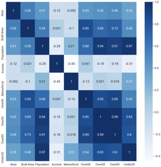
Figure 1.
Correlation between socioeconomic features.
We can observe moderate correlations between the basic features: area, population, and built area. Not very surprisingly, there are also higher correlations between the features regarding the age structure.
It can also be observed that POPULATION and BUILTAREA correlate with the age structure. More precisely, POPULATION is strongly correlated with UNDER_20, OVER_50, and OVER_65, and BUILTAREA is correlated strongly with OVER_85. This holds because all these features correspond to the size of a country. If the population or the built-up area of a country is large, then the absolute number of people of a certain age is also large.
Income and secondary education have a moderate negative correlation and are not strongly correlated with any of the other values.
The correlations between different waste types are shown in Figure 2.
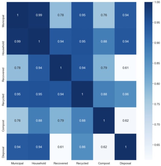
Figure 2.
Correlation between different waste types.
Two different classes of waste types can be distinguished. On the one hand, waste production can be associated with municipal, household, and disposal waste. By contrast, recovered, recycled, and compost waste correspond to waste reuse. The heat map shows that the correlation within these two clusters are very high. In addition, municipal waste, which comprises total waste, is highly correlated with all other waste types.
Finally, we can calculate the correlations between socioeconomic features and waste types. As can be seen in Figure 3, some of the socio-economic features correlate very strongly with waste production. In particular, built area seems to have a high impact on all waste types. In addition, population size has a rather strong impact on the waste production. On the other hand, income does not seem to have much influence on the waste numbers.
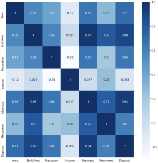
Figure 3.
Correlation between selected socio-economic features and selected waste types.
4. Data Analytics Methods
This section summarizes the selected ML algorithms used for prediction and clustering and also the evaluation metrics applied to determine the performance errors produced by the ML algorithms.
4.1. Selected Machine Learning Algorithms
This subsection describes the selected ML regression algorithms used to predict annual solid waste production by countries—in particular, Support Vector Regressor, Gradient Boosting Regressor, and Random Forest Regressor, respectively. Next, we describe k-means as the method to perform unsupervised clustering by countries.
4.1.1. Support Vector Regression
Support Vector Regression (SVR) [30,31] uses the same principles as Support Vector Machines (SVM) for classification with minor differences, since in regression problems, the outputs are real numbers. Given a set of n training data where represent the input variables, represents the outputs to be approximated, and m is the dimension of input variables. The SVR algorithm searches a function that has at most an deviation from the searched targets for all the training data:
such that each element is placed to a maximal distance from computed . At the same time, as function defines a hyperplane, we search the corresponding one to minimize the norm of w (i.e., flatness property). The problem can be written as a convex optimization one:
The assumption of the previous equation is that function exists and it approximates all pairs with a precision (i.e., the convex optimization problem is feasible). As it could not be the case, we may allow some errors represented by slack variables , and the last equation can be rewritten as:
where the constant represents a trade-off between the flatness of and the amount up to which deviations larger than are tolerated.
When data are not linearly separable in the original space, these are projected into a higher-dimensional space using a kernel function K (mainly linear, polynomial, or Gaussian). The previous equation is rewritten as:
Note that in this problem we have two parameters: and C. The first one represents the maximum error deviation assumed for all training data, and C represents the importance of accumulated errors in the optimization problem.
4.1.2. Gradient Boosting Regressor
Like Gradient Boosting (GB), the Gradient Boosting Regressor (GBR) [30] uses a combination of multiple weak decision trees (i.e., weak regressors) into a single composite algorithm to approximate the function , given the set of n training data . The GBR algorithm has M stages () which correspond to the number of decision trees (i.e., estimators) used. At each stage, a new decision tree is computed from the previous one as follows:
The residual represents the difference between desired result and previous model. To initialize the algorithm, the initial model is set as . It is necessary to include the parameter r that represents the importance given to each estimator. Finally, the resulting GBR model is computed as:
4.1.3. Random Forest Regressor
Random Forest Regressor (RFR) [30,31] builds multiple decision trees at training and merges them together to obtain a more accurate and stable prediction. A random forest is a meta-estimator that fits a number of classifying decision trees on various sub-samples of the dataset and uses mean averaging to improve the predictive accuracy and control over-fitting.
Feature or node importance is computed as the decrease in node impurity weighted by the probability of the node. The tree node probability can be estimated by the number of data that reach that node divided by the total number of data.
For each decision tree, the node importance can be calculated using Gini importance. In the case of a binary tree:
where is the importance of node j, and are, respectively, the weighted number of data samples reaching left child and right child of node j; and and are, respectively, the Gini impurity values of left child and right child of node j.
The importance for each feature on a decision tree is then calculated as:
where is the importance of feature i and is the importance of node j.
These importance values can be normalized (between 0 and 1) by dividing them by the sum of all feature importance values:
The predicted final feature importance at the Random Forest level is computed as the average of all the trees as follows:
where is the importance of feature i computed for all the trees in the Random Forest, is the normalized feature importance for feature i in tree j, and T is the total number of trees.
4.1.4. Clustering: k-Means Algorithm
Clustering [32] is a non-supervised machine learning task that involves the automatic discovering of groups (or clusters) from multi-dimensional data in a feature space. Clustering algorithms are generally divided into hierarchical and non-hierarchical ones. Hierarchical methods seek to build a hierarchy (i.e., tree) of clusters using an agglomerative or a divisive strategy. Non-hierarchical clustering involves the creation of new clusters by merging or splitting the existing ones without following a tree-like structure. Hierarchical clustering presents the advantage that the number of clusters is not required, and it is also easy to implement. However, the time complexity of most of the hierarchical clustering algorithms is quadratic, i.e., . One of the most popular non-hierarchical clustering methods is k-means [32], which is linear in the number of patterns n to be classified, i.e., .
The k-means algorithm is applied to partition a set of patterns into a given number of k clusters . The algorithm starts with a random selection of the k centroids of clusters (). During each update step (or iteration) t, all patterns x are assigned to their nearest centroid. When a given pattern has the same distance to multiple centroids, a random one is chosen.
Then, these centroids are recalculated at by computing the mean of the assigned patterns into each cluster:
The update process repeats until all patterns in an iteration remain at the same class that in the previous iteration. Consequently, the centroids positions would not require to be updated anymore.
4.2. Evaluation Metrics
In this paper, we have considered the following statistical metrics to evaluate the performance capabilities of the compared algorithms: Root Mean Square Error (RMSE), Mean Absolute Error (MAE), Mean Absolute Percentage Error (MAPE), and coefficient of determination (),
These metrics are defined and formulated as follows, where W, , and n, respectively, represent the real generated waste, the predicted waste by the algorithm, and the number of observations.
RMSE is a widely used metric for regression tasks. The errors are first squared before averaging, which yields high penalties on large errors. RSME is especially meaningful when large errors are undesired.
MAE represents the average of the absolute difference between the actual and predicted values in the dataset, and it measures the average of the residuals in the dataset. MAE weights all individually differences equally and is more robust to outliers. It does not penalize outliers as much as RSME.
MAPE relates MAE to the size of the target values. It facilitates the understanding of the prediction accuracy when measures of different scales are considered. Since the different waste measures have different magnitudes, we often use MAPE below to provide an integrated picture of prediction accuracy across all waste types.
represents the proportion of the variance in the dependent variable which is explained by the linear regression model, and it is a scale-free score. The metric helps to compare the prediction to a constant baseline, which is given by the mean of the data. If the sum of Squared Error of the regression line is small, then is close to 1.
5. Analysis of the OECD Data
In this section, we apply the ML methods presented in Section 4 for analyzing the country-specific waste production. In particular, we address the following goals:
- clustering of countries based on their socio-economic features as well as their waste production;
- predicting the waste data from socio-economic data applying ML methods;
- comparing the performance of the different ML methods;
- fine-tuning the prediction models by optimizing the hyperparameters;
- analyzing the importance of the particular features.
Our data analysis is performed with Scikit-learn, the well-known open source Python ML library, which provides various classification, regression, and clustering algorithms. Our models are also using further libraries such as Pandas and NumPy for data wrangling and Matplotlib for plotting. All data and the code in form of Jupyter notebooks are available at https://sync.academiccloud.de/index.php/s/ltio2QthmpnKXQV (accessed on 10 January 2022).
5.1. Clustering Countries
In this subsection, we cluster the different countries according to their waste consumption and their socio-economic features, respectively. Clustering is the task of partitioning the dataset into groups, the so-called clusters. The goal is to split up the data in such a way that data points within a single cluster are very similar and data points in different clusters are different.
5.1.1. Pre-Processing
In order to cluster the countries according to the given OECD data, we need to perform some pre-processing steps. To make countries of different sizes comparable, we calculate the waste production per capita. Furthermore, we scale the data with a MinMax scaler to deal with features of different orders of magnitude.
5.1.2. Clustering Algorithm
For the clustering algorithm, we have chosen k-means, which is one of the simplest and most commonly used clustering methods.In addition, we applied also agglomerative clustering, which produces more or less the same results.
A major challenge for k-means clustering is to determine how many clusters the algorithm should create. For determining the optimal number of clusters, we applied the popular elbow method that is implemented by the KneeLocator in Scikit-learn. The KneeLocator evaluates the quality of a certain cluster by the sum of squared errors (SSE), i.e., the squared distance of each point to their respective cluster centroid.
5.1.3. Results
Our goal is to find clusters for all countries given in the OECD dataset due to their waste production. The features we used for clustering are waste production per capita of all waste types. This allows us to group countries with similar waste consumption behavior. If we would have used absolute waste quantities instead, countries would have been grouped according to their size. As the result of our KneeLocator analysis we received an optimal number of four clusters.
Considering four clusters for the year 2017, it separates the countries mainly in the following groups:
- Cluster 1: it contains only the USA, which plays a special role because it has by far the highest percentage of disposal waste and the second highest value of municipal waste;
- Cluster 2: Slovac Republic, Turkey, and Costa Rica. These are the three countries with the lowest number for recovered waste;
- Cluster 3: it contains the wealthy European countries of great economic strength such as Austria, Denmark, Germany, Luxembourg, Netherlands, Norway, and Switzerland. These countries tend to produce the most municipal and household waste per capita but also recycle the most waste;
- Cluster 4: it contains most of the other European countries, such as Czech Republic, France, UK, France, and Ireland, but also Japan and Korea. The waste volumes of these countries do not show any extremes and are in a rather medium range.
Note that many countries changed their cluster at least once between 1999 and 2017.
5.2. Predicting Waste
A main objective of this work is to investigate how socio-economic, free available open-access data can be used to predict a country’s waste production. Following the ML approach, we want to find a prediction (or hypothesis) function h:
where is the i-th feature vector in the dataset (i.e., the vector of the socio-economic features of a particular county in a year, and the corresponding predicted value, i.e., the quantity of a particular type of waste generated in a certain country in a given year. The hypothesis function can be considered as the prediction model we have learned.
Waste prediction can be considered as a regression task, since the goal is to predict a continuous number, namely the quantity of waste production.
According to the ML process, we proceed the following steps for finding an appropriate :
- Feature engineering:In the first step, we have to select the set of features we want to use for learning an appropriate prediction function. In particular, we have to take the data quality of the given data into account. If instances in the dataset are missing a few features, we must decide whether to ignore this feature altogether, ignoring these instances or trying to fill the missing data.Some of the ML methods, such as SVR or Gradient Boosting do not perform well with input data of different scales. Then, the data must be scaled by using a scaling method such as standard min-max scaling. Other methods, for instance, tree-based methods such as Random Forest, also work without a scaling step;
- Splitting data into training and test set:After preparing the data, we split it applying standard K-fold cross-validation and use 15% of the dataset for testing and evaluating our prediction model. In our experiments shown below, we used folds throughout;
- Model selection and training:The next step is to select a suitable prediction model to train on the dataset. We conducted several experiments with different models and evaluated how well each model performed. For each model, we performed a grid search to optimize the specific hyper-parameters to improve its performance. This means that we tried out systematically different combinations of the specific model parameters;
- Model evaluation:Finally, we evaluated the predictive quality of our model by applying it to the test dataset. We measured the differences between the predicted values and the target values, i.e., the real waste quantities reported by the OECD using the metrics presented in Section 4.2.
5.2.1. Predicting Waste Based on Socio-Economic Data
First, we examine how good waste can be predicted from socio-economic OECD data. The targets to predict are the absolute waste quantities for the six given waste types: municipal, household, recovered, recycled, compost, and disposal. Data instances that do not have an entry for this target have to be deleted from both the training and test datasets. As shown in Table 3, this can reduce the dataset size significantly. For instance, only 54% of the OECD data instances have data on household waste.
Then, for each target, we trained a selected model and fine-tuned its hyper-parameters using a GridSearch.
Feature Engineering
Our prediction model should be based on all given socioeconomic data of a country. The considered features are: ‘Area’, ‘Built’, ‘Built Area’, ‘Population’, ‘Income’, and all attributes indicating the different age groups. In addition, we have added one-hot encoding to the country feature so that we can track to which country a data instance belongs to.
As considered in Section 3.2, we removed features with too many missing values, such as MEDIAN_INCOME and BELOW_SCND from the dataset.
Model Selection
For predicting the waste quantities, we experimented with various regression models—among others, Support Vector Regression (SVR), Gradient Boosting (GB), and Random Forest Regressor (RFR) (see Section 4). We also tried Gaussian Process Regressor (GPR), but it did not produce reasonable results. Therefore, we refrain from presenting the results. Note that these methods except RandomForest require a scaling step before training on the dataset. We applied standard min-max scaling.
The following two tables show the prediction errors of the chosen Machine Learning methods for two waste types. Table 4 presents the results for municipal waste. Regarding the metrics and MAPE, all methods perform very well. Overall, Random Forest seems to performs slightly better. Furthermore, we can see that the RMSE value of Gradient Boosting is the lowest, so it can handle outliers best. Altogether, we can consider RFR and GB as the most suitable methods.
Table 4.
Prediction errors of different ML methods for municipal waste.
Considering the recovered waste, we obtain completely different results, as shown in Table 5. RFR outperforms by far the other methods. Note that the RMSE and MAE are much smaller than in Table 4, because the absolute number of recovered waste are much smaller than that of municipal waste.
Table 5.
Prediction errors of different ML methods for recovered waste.
In summary, our results show that RFR provides by far the best results. SVR and GBR also yield excellent results for municipal and household waste, but they do not produce stable results for the other waste types. Therefore, we conduct all experiments with RFR in the following section.
Results for Random Forest
The following Table 6 presents the prediction errors for the different waste types when using Random Forest Regression.
Table 6.
Random Forest Regression: prediction errors for different waste types based on socio-economic data.
We calculated the and MAPE metrics for the test dataset. As Table 6 illustrates, Random Forest Regression yields very good results. In particular, the predictions for municipal, household, and disposal waste are very accurate. For instance, the mean absolute percentage error (MAPE), which can be easily interpreted, ranges between 3% and 9% for municipal, household, and disposal waste.
However, the other waste types (recovered, recycled, and compost) MAPE errors are between 21% and 30%. These significantly worse prediction results are due to poorer data quality. For instance, if we look at the predictions of the recycled waste in the test dataset, we see that the majority of the predictions is still excellent. However, there are few outliers that have big impact on the average prediction quality.
Let us consider an extreme example: for Lithuania, the amount of recycled waste in the year 2006 reported by the OECD was 14, but the predictor calculates a value of 80, which yields a MAPE of 417%. Looking at the data for Lithuania provided by the OECD, we obtain the following curve, shown in the Figure 4.
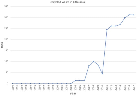
Figure 4.
OECD data for the recycled waste in Lithuania from 1990 to 2017.
We can observe large discontinuities between the values. Until 2003, the recycled waste was not measured. From 2004 to 2006, the quantity was constant at 14 tons, and then within one year, it jumped to 80 tons, an increase of 471%. Similar jumps can be seen between the years 2008 and 2011. Such an erratic course cannot be predicted with high accuracy, and the predictor comes to its limits. In these cases, however, it can be doubted whether the OECD data are correct. Probably, the large jumps do not mean large changes in the waste produced but in how the data were collected.
One approach to dealing with poor data quality would be detecting outliers: data instances involved in large jumps should be removed from the dataset. We have decided not to do this, because the size of the dataset is already very small. Fortunately, the newer data seem to be much better; therefore, we can hope that the prediction accuracy will improve in the future especially for countries with still poor data quality.
What we can also report are the values for the optimal hyper-parameters of the Random Forest Regressor, which are shown in Table 7.
Table 7.
Hyper-parameters of Random Forest Regression found by GridSearch.
Using GridSearch, we obtained specific hyper-parameters for each type of waste in our experiments. Random Forest models are an ensemble of decision trees; therefore, we can specify the number of decision trees in the forest. In our experiments, the optimal number varies between 8 and 15, depending on the waste type. Max_features is the number of features to resample. In Scikit-learn, ‘auto’ defines no restrictions on the number of features, and ‘sqrt’ means that not more than the square root of the total number of features can be used. The parameter minimum sample split specifies the minimum number of samples required to split an internal leaf node.
Feature Importance
When deriving a prediction model, we are interested not only in its accuracy but also in understanding how the predictions are inferred. When using decision trees, we can calculate the feature importance that rates how important each feature is for constructing the tree. Permutation feature importance calculates the increase in the model’s prediction error after permuting a feature. If shuffling the values of that particular feature results in a significantly larger model error, then the model has relied on that feature, which can be considered important. If the model error remains unchanged by the shuffle, the model ignores that feature for prediction. The feature importance values sum up to one and describe how much a certain feature contributes to the prediction. Thus, a feature-importance value can be viewed as a percentage expressing the importance of that feature.
Feature importance helps us to understand which features are mainly used in the prediction and may allow us to reduce the feature space, making the model training much faster. The importance of features depends strongly on the the type of waste, as Figure 5 shows.
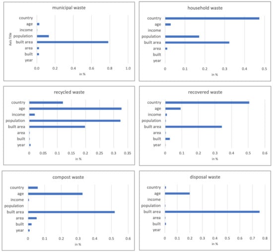
Figure 5.
Importance of different socio-economic features.
In general, the feature BUILT AREA, which is the absolute area in a country, which contains any kind of buildings, has the greatest influence on waste quantities. This features corresponds to the size of a country and its industrial strength, which obviously have a particularly strong influence on waste production.
It can also be noted that the feature COUNTRY is very important for some waste types, namely household waste and recycled waste. Since this feature was modeled by one-hot encoding, it is in fact implemented by 43 Boolean features. A closer look at the data shows us that some of these features are of high importance. For instance, the feature that denotes that a data instance belongs to the USA is of high importance for predicting the household waste. This means that for household waste, the course of waste quantities behave differently for various countries. Therefore, the predictor is not generalizable to all countries but must be country specific to provide accurate results. Note that there are only a few countries that require this special treatment.
It is also interesting to note that income does not play an important role in predicting waste, but age structure has a significant impact on predicting recycled, composted, and disposed waste.
5.2.2. Predicting Waste from Other Waste Types
Finally, we investigate how a particular waste type can be predicted when the waste production quantities of all other waste types are given. This means that we use only five waste types as features: those types that are different to the target waste type.
Model Selection
Again, we compare the performance of our chosen ML methods for the municipal waste and for recovered waste. We obtain very similar results to those in the previous section, where we predicted waste production using socio-economic features. All ML methods perform excellently for municipal waste as Table 8 shows.
Table 8.
Prediction errors of different ML methods for municipal waste based on other waste types.
As in the previous section, we find that for recycled waste, Random Forest far outperforms Support Vector Regression and Gradient Boosting, especially when considering MAPE metrics (shown in Table 9). Therefore, we stick to Random Forest Regression in the following.
Table 9.
Prediction errors of different ML methods for recovered waste based on other waste types.
Results with Random Forest
The results depicted in Table 10 show similar results as in the previous experiments. This means that even if we know only four of the five waste production quantities, we can predict the missing quantity.
Table 10.
Random Forest Regression: prediction errors for each waste type based on other waste types.
Also shown in this experiment, waste predictions for municipal and household are excellent. For all other waste types, the prediction model yields reasonable results on average. Looking at our test data in detail, we can observe that most of the predictions are very accurate, but some outliers are responsible for the worse results on average.
These outliers can be related to countries where the course of the waste data makes large jumps that do not seem to correspond to reality. Such erratic behavior cannot be accurately predicted by ML methods. Once again, the quality of the data is responsible for the accuracy of our predictions.
Figure 6 shows the course of the waste data for Estonia and France as an example.
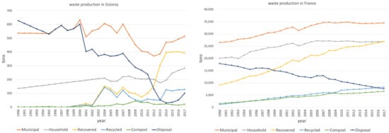
Figure 6.
Course of the OECD waste data for selected countries: Estonia and France.
For France, on the right-hand side, we see smooth changes in the waste quantities of all types, which can be precisely predicted. However, the data for Estonia on the left show strange jumps of over 100% from one year to the next. For instance, recycled waste between 2002 and 2014 forms a zigzag curve that cannot be predicted correctly.
Considering all OECD waste data, we can observe that data on reused waste is not of the same quality as municipal and household data. This affects the prediction accuracy significantly, as shown in Table 10.
Feature Importance
In addition, in this experiment, it is interesting to look at the importance of the features used. Figure 7 shows the features for each of our prediction models.
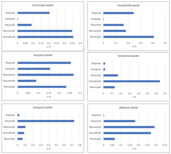
Figure 7.
Feature importance of different waste types.
We can see that municipal and household waste is of high importance in most most models. It can be assumed that the values of these two waste types generally characterize the waste production of a country.
The only exception is the model for compost waste, which is strongly influenced by the recycled waste. Here, it can be speculated that the value of the compost waste is more influenced by the recycled waste, which might characterize the reuse of waste in general. On the other side, we can see that the compost feature is almost insignificant for all features except the recycled waste.
Feature importance is related to the results of our co-variance analysis in Section 3.3, in particular the correlations shown in Figure 2. Features with high correlation show stronger linear dependence and hence have almost the same effect on the target feature. Thus, out of the two highly correlated features, only one has high feature importance. On the other hand, a feature with a low feature importance could be highly correlated to the target. This just means that it was not used when constructing the model, because another feature contains the same information.
6. Conclusions
In this work, we investigated the potential of using open data to analyze waste. Multiple experiments were conducted to predict different types of solid waste for OECD countries from 1990 to 2017 using different ML models. Furthermore, cluster analysis was applied to determine similarities among groups of countries presenting similar waste production and recycling characteristics.
The main contributions of this work are: (1) a waste analysis at the OECD country-level, which allows one to compare and cluster countries according to similar waste and socio-economic features; (2) the in-depth analysis of a set of open demographic and socio-economic data to identify the key features that can be used to train ML models (in particular, the quality and usefulness of the open data provided is discussed in detail); and (3) a comparison of different ML regression methods under the same metrics according to their prediction capabilities.
In the performed experiments, we addressed the following goals: clustering of countries based on their socio-economic features as well as their waste production; predicting the waste data from socio-economic data applying ML methods; comparing the performance of the different ML methods and fine-tuning the prediction models by optimizing the model hyperparameters; and analyzing the importance of the particular features. The experiments we conducted have shown that ML methods such as Random Forest Regressor (RFR) can provide very accurate results for waste prediction even based on open data.
The main limitation of our approach is the availability and quality of the available data. As explained in detail in Section 3 and Section 6, the OECD dataset has several shortcomings. On the one hand, plenty of data was missing and was imputed to fill the gaps. Of course, more realistic results could be achieved with a complete set of data. In addition, for some of the OECD countries, there are irregular patterns with large discontinuities in the data as shown in Figure 4 for the recycled waste in Lithuania. Such large jumps in the data do not correspond to the real situation and cannot be accurately predicted. Furthermore, waste analysis could provide more insights if more socio-economic features were available, which unfortunately are not included in the OECD dataset. For instance, it would be interesting to know about the size of households or the proportion of people living in rural or urban areas or climatic conditions. More detailed data from smaller and more homogeneous neighborhoods could also provide more insights into the key factors influencing waste generation.
Future research directions in this work can consist in testing new advanced ML algorithms using Deep Learning—in particular, networks based on Long Short-Term Memory (LSTM) models, which have produced very good results in some predictive problems such as handwritten text recognition or pedestrian trajectory prediction. It is also interesting to remark that performance of considered prediction algorithms depends on the parameters setting of the models. In consequence, it can be convenient to optimize these model parameters using heuristic techniques such as Genetic Algorithms or Particle Swarm Optimization.
Author Contributions
All the authors contributed equally throughout the entire process of completing the research. J.D., Á.S., Ó.G.B. and D.D. conceived the study and were responsible for the methodology, and development of the data analysis. J.D., Á.S., Ó.G.B. and D.D. were responsible for the data collection, preparation and experiments. J.D., Á.S., Ó.G.B. and D.D. wrote the first draft of the article, reviewed and interpreted the results, and they are responsible for the data interpretation. All authors have read and agreed to the published version of the manuscript.
Funding
This work was funded by the Spanish Ministry of Science and Innovation projects with Grants No.: RTI2018-098019-B-I00 and PID2020-114867RB-I00; and by the CYTED Network “Ibero-American Thematic Network on ICT Applications for Smart Cities” with Grant No.: 518RT0559.
Institutional Review Board Statement
Not applicable.
Informed Consent Statement
Not applicable.
Data Availability Statement
All data generated or analyzed during this study are included in this published article.
Conflicts of Interest
The authors declare no conflict of interest.
Abbreviations
The following abbreviations are used in this manuscript:
| OECD | Organisation for Economic Co-operation and Development |
| SWM | Solid Waste Management |
| SC | Smart City |
| ML | Machine Learning |
| AI | Artificial Intelligence |
| SVR | Support Vector Regressor |
| GBR | Gradient Boosting Regressor |
| RFR | Random Forest Regressor |
| MAE | Mean Absolute Error |
| RMSE | Root Mean Square Error |
| MAPE | Mean Absolute Percentage Error |
References
- The World Bank. Solid Waste Management. 2019. Available online: https://www.worldbank.org/en/topic/urbandevelopment/brief/solid-waste-management (accessed on 15 January 2021).
- Abbasi, M.; El Hanandeh, A. Forecasting municipal solid waste generation using artificial intelligence modelling approaches. Waste Manag. 2016, 56, 13–22. [Google Scholar] [CrossRef]
- Beigl, P.; Lebersorger, S.; Salhofer, S. Modelling municipal solid waste generation: A review. Waste Manag. 2008, 28, 200–214. [Google Scholar] [CrossRef] [PubMed]
- Keser, S.; Duzgun, S.; Aksoy, A. Application of spatial and non-spatial data analysis in determination of the factors that impact municipal solid waste generation rates in Turkey. Waste Manag. 2012, 32, 359–371. [Google Scholar] [CrossRef] [PubMed]
- Antanasijevic, D.; Pocajt, V.; Popovic, I.; Redzic, N.; Ristic, M. The forecasting of municipal waste generation using artificial neural networks and sustainability indicators. Sustain. Sci. 2013, 8, 37–46. [Google Scholar] [CrossRef]
- Cubillos, M.; Wulff, J.N.; Wøhlk, S. A multilevel Bayesian framework for predicting municipal waste generation rates. Waste Manag. 2021, 127, 90–100. [Google Scholar] [CrossRef] [PubMed]
- Marquez, M.Y.; Ojeda, S.; Hidalgo, H. Identification of behavior patterns in household solid waste generation in Mexicali’s city: Study case. Resour. Conserv. Recycl. 2008, 52, 1299–1306. [Google Scholar] [CrossRef]
- Abdallah, M.; Talib, M.; Feroz, S.; Nasir, Q.; Abdalla, H.; Mahfood, B. Artificial intelligence applications in solid waste management: A systematic research review. Waste Manag. 2020, 109, 231–246. [Google Scholar] [CrossRef] [PubMed]
- Kolekar, K.; Hazra, T.; Chakrabarty, S.N. A Review on Prediction of Municipal Solid Waste Generation Models. Procedia Environ. Sci. 2016, 35, 238–244. [Google Scholar] [CrossRef]
- Solano-Meza, J.K.; Orjuela, D.; Rodrigo-Ilarri, J.; Cassiraga, E. Predictive analysis of urban waste generation for the city of Bogotá, Colombia, through the implementation of decision trees-based machine learning, support vector machines and artificial neural networks. Heliyon 2019, 5, e02810. [Google Scholar] [CrossRef]
- Cubillos, M. Multi-site household waste generation forecasting using a deep learning approach. Waste Manag. 2020, 115, 8–14. [Google Scholar] [CrossRef]
- Azevedo, B.D.; Scavarda, L.F.; Caiado, R.G.G.; Fuss, M. Improving urban household solid waste management in developing countries based on the German experience. Waste Manag. 2021, 120, 772–783. [Google Scholar] [CrossRef]
- Thanh, N.; Matsui, Y.; Fujiwara, T. Household solid waste generation and characteristic in a Mekong Delta City, Vietnam. J. Environ. Manag. 2010, 91, 2307–2321. [Google Scholar] [CrossRef]
- Noori, R.; Abdoli, M.; Farokhnia, A.; Abbasi, A. Results Uncertainty of Solid Waste Generation Forecasting by Hybrid of Wavelet Transform-ANFIS and Wavelet Transform Neural Network. Expert Syst. Appl. 2009, 36, 9991–9999. [Google Scholar] [CrossRef]
- Kontokosta, C.E.; Hong, B.; Johnson, N.E.; Starobin, D. Using machine learning and small area estimation to predict building-level municipal solid waste generation in cities. Comput. Environ. Urban Syst. 2018, 70, 151–162. [Google Scholar] [CrossRef]
- Kulisz, M.; Kujawska, J. Prediction of Municipal Waste Generation in Poland Using Neural Network Modeling. Sustainability 2020, 12, 10088. [Google Scholar] [CrossRef]
- Ramasami, K.; Velumani, B. Location prediction for solid waste management—A Genetic algorithmic approach. In Proceedings of the IEEE International Conference on Computational Intelligence and Computing Research (ICCIC 2016), Chennai, India, 15–17 December 2016; pp. 1–5. [Google Scholar]
- Basri, H.B.; Stentiford, E.I. Expert Systems in Solid Waste Management. Waste Manag. Res. 1995, 13, 67–89. [Google Scholar] [CrossRef]
- Kolekar, K.; Hazra, T.; Chakrabarty, S.N. Prediction of municipal solid waste generation for developing countries in temporal scale: A fuzzy inference system approach. Glob. Nest J. 2017, 19, 511–520. [Google Scholar]
- Goel, S.; Ranjan, V.; Bardhan, B.; Hazra, T. Forecasting Solid Waste Generation Rates. In Modelling Trends in Solid and Hazardous Waste Management; Sengupta, D., Agrahari, S., Eds.; Springer: Singapore, 2017; pp. 35–64. [Google Scholar]
- Magazzino, C.; Mele, M.; Morelli, G.; Schneider, N. The nexus between information technology and environmental pollution: Application of a new machine learning algorithm to OECD countries. Util. Policy 2021, 72, 101256. [Google Scholar] [CrossRef]
- Guo, H.; Wu, S.; Tian, Y.; Zhang, J.; Liu, H. Application of machine learning methods for the prediction of organic solid waste treatment and recycling processes: A review. Bioresour. Technol. 2021, 319, 124114. [Google Scholar] [CrossRef]
- Abualigah, L. Feature Selection and Enhanced Krill Herd Algorithm for Text Document Clustering; Studies in Computational Intelligence; Springer Nature Switzerland AG: Berlin, Germany, 2019; pp. 1–165. [Google Scholar]
- Abualigah, L.; Elaziz, M.A.; Sumari, P.; Geem, Z.W.; Gandomi, A.H. Reptile Search Algorithm (RSA): A nature-inspired meta-heuristic optimizer. Expert Syst. Appl. 2022, 191, 116158. [Google Scholar] [CrossRef]
- Guleryuz, D. Evaluation of waste management using clustering algorithm in megacity Istanbul. Environ. Sci. Technol. 2020, 3, 10–112. [Google Scholar]
- Agovino, M.; Ferrara, M.; Garofalo, A. An exploratory analysis on waste management in Italy: A focus on waste disposed in landfill. Land Use Policy 2016, 57, 669–681. [Google Scholar] [CrossRef]
- Caruso, G.; Gattone, S.A. Waste Management Analysis in Developing Countries through Unsupervised Classification of Mixed Data. Soc. Sci. 2019, 8, 186. [Google Scholar] [CrossRef] [Green Version]
- Sharma, N.; Litoriya, R.; Sharma, A. Application and Analysis of K-Means Algorithms on a Decision Support Framework for Municipal Solid. In Proceedings of the International Conference on Advanced Machine Learning Technologies and Applications, Cairo, Egypt, 28–30 March 2020; pp. 267–276. [Google Scholar]
- Otoo, D.; Amponsah, S.K.; Sebil, C. Capacitated clustering and collection of solid waste in Kwadaso estate. Asian J. Sci. Res. 2014, 4, 460–472. [Google Scholar]
- Bowles, M. Machine Learning in Python: Essential Techniques for Predictive Analysis; John Wiley & Sons Inc.: Indianapolis, IN, USA, 2015. [Google Scholar]
- Rodriguez-Galiano, V.; Sanchez-Castillo, M.; Chica-Olmo, M.; Chica-Rivas, M. Machine learning predictive models for mineral prospectivity: An evaluation of neural networks, random forest, regression trees and support vector machines. Ore Geol. Rev. 2015, 71, 804–818. [Google Scholar] [CrossRef]
- Wu, J. Advances in K-Means Clustering: A Data Mining Thinking; Springer: Berlin/Heidelberg, Germany, 2012; pp. 1–180. [Google Scholar]
Publisher’s Note: MDPI stays neutral with regard to jurisdictional claims in published maps and institutional affiliations. |
© 2022 by the authors. Licensee MDPI, Basel, Switzerland. This article is an open access article distributed under the terms and conditions of the Creative Commons Attribution (CC BY) license (https://creativecommons.org/licenses/by/4.0/).