An Efficient Wireless Sensor Network Based on the ESP-MESH Protocol for Indoor and Outdoor Air Quality Monitoring

Abstract

The main aim of this work is to establish a sensor MESH network using an ESP-MESH networking protocol with the ESP32 MCU (a Wi-Fi-enabled microcontroller) for indoor and outdoor air quality monitoring in real time. Each sensor node is deployed at a different location on the college campus and includes sensor arrays (CO₂, CO, and air quality) interfaced with the ESP32. The ESP-MESH networking protocol is a low-cost, easy-to-implement, medium-range, and low-power option. ESP32 microcontrollers are inexpensive and are used to establish the ESP-MESH network that allows numerous sensor nodes spread over a large physical area to be interconnected under the same wireless network to monitor air quality parameters accurately. The data of different air quality parameters (temperature, humidity, PM2.5, gas concentrations, etc.) is taken (every 2 min) from the indoor and outdoor nodes and continuously monitored for 72 min. A custom time-division multiple-access (TDMA) scheduling scheme for energy efficiency is applied to construct an appropriate transmission schedule that reduces the end-to-end transmission time from the sensor nodes to the router. The performance of the MESH network is estimated in terms of the package loss rate (PLR), package fault rate (PFR), and rate of packet delivery (RPD). The value of the RPD is more than 97%, and the value of the PMR and PER for each active node is less than 1.8%, which is under the limit. The results show that the ESP-MESH network protocol offers a considerably good quality of service, mainly for medium-area networks.

1. Introduction

The oxygen present in the air is essential for human life. The air combines oxygen, nitrogen, inert gases, and water vapor. In the atmosphere, human actions release unwanted elements, some of which could be the source of complications for living beings (plants, humans, and animals). Polluted air also affects plant growth in precision agriculture [1].

Air quality could be articulated by the absorption of numerous pollutants, such as carbon NOx, SO₂, O₃, CO, HC, volatile or semi-volatile organic compounds (VOCs), and particulate matter (PM) of diverse particle sizes [2]. The level of air pollution could also be expressed in terms of the air quality index (AQI) [3].

Contamination inside our homes is also considered an alarming issue, as well in offices and schools. Indoor actions, such as smoking and cooking, could create impurities. Typically, in manufacturing nations, the inhabitants devote approximately 80–90% of their time inside houses and are consequently exposed to detrimental interior contaminants. Indoor air quality is commonly evaluated by distinctly gauging the CO, temperature, and humidity [4]. These statistics, even if merged, are deficient in permitting a good depiction of the inside air quality.

There are mainly two types of outdoor air pollutants in urban areas: vehicle emissions and industrial emissions. Depending on the location and winds, there could also be contributions from power plants and industrial boilers, incinerators, petrochemical plants, aircraft, and ships [2,5].

Numerous studies [6,7,8] indicated that outdoor air influences indoor air quality. Kuo and Shen et al. [6] found a similar increase in PM2.5 and PM10 concentrations indoors and outdoors during a dust storm event, which they attributed to the ventilation system’s extraction of outdoor air.

The effects of poor air quality could be felt immediately, even after exposure to pollutants only, including irritation of the throat, eyes, and nose, a headache, and so on [9]. For monitoring the air pollution effects in homes and workplaces before the condition becomes more serious, a real-time air quality monitoring system is quickly becoming necessary.

Indoor and outdoor air quality monitoring networks characterized by high flexibility and a real-time, modular, and cost-effective nature are becoming feasible due to the advancement of IoT technology, information communication technology (ICT), and sensor technology [10]. In [11], Kumar et al. proposed an inexpensive indoor pollution gas monitoring system based on internet of things (IoT) technology to monitor indoor air quality. Many researchers have already addressed this issue. An integrated DSP microcontroller was used for this monitoring system, allowing it to measure CO and CO₂ gas concentrations with a deviation of ±5% from the standard data set.

Using WSNs, Abraham and Li proposed an inexpensive IAQ monitoring system [12] that could simultaneously collect six air quality parameters from various sites. A real-time system for monitoring CH₄ and CO gases was proposed by Ahmed et al. in [13], but the final system cost increased due to the Intel Edison microcontroller board. Firdhous et al. in [14] projected an inside air monitoring system, which was imperfect for O₃ only, based on the IoT technology.

After reviewing the available literature, it was recognized that communication technologies mostly used Bluetooth low energy (BTLE), Wi-Fi, and Zig-Bee [15,16,17].

Hence, an inexpensive and medium-range network was proposed to measure indoor and outdoor air quality. For this, a dust and gas sensor was used to monitor the PM2.5 dust particles and toxic gases. Scientists have long pointed out that haze could significantly increase lung cancer risk, reducing the average life expectancy by one year [18]. MQ series gas sensors (MQ-135, MQ-2, and MQ-7) are available for monitoring air quality (benzene, alcohol, and NH₃), methane, butane, LPG, smoke, and carbon monoxide.

Finally, temperature and humidity sensors are selected so that people can monitor how comfortable their working and living environments are and how the temperature and humidity impact other parameters.

This work aims to present an indoor and outdoor air quality monitoring system by using an ESP-MESH networking protocol that permits abundant devices (stated as sensor nodes) spread over a large physical area (both indoors and outdoors) to be consistent under one WLAN (wireless local-area network) for a precise extent of air quality and the recognition of the air contamination measures of the sensor’s irregular operation. The main influence of this article is as follows:

• As part of the first step, the hardware platform for the air quality sensors, which includes a gateway, a base station, and sensors, is designed; specifically, a new hardware platform for the sensor nodes that could collect air quality measurements from the indoors and outdoors;
• The second function of the system software is to provide data acquisition, processing, transmission capabilities, and energy conservation strategies for the entire system;
• Third, utilizing a custom time-division multiple-access (TDMA) scheduling scheme for energy efficiency, a transmission schedule that reduces the end-to-end transmission time from the sensor nodes to the router is constructed;
• Fourth, the experimentation of the sensor accurateness extent in the real physical scenes is provided;
• In the final section, we evaluate the communication interface performance, including the package loss rate (PLR), package fault rate (PFR), and rate of packet delivery (RPD).

2. ESP-MESH Protocol

Based on a Wi-Fi protocol, a novel networking protocol, “ESP-MESH”, was proposed by Espressif Systems (Shanghai, China) CO., LTD [19].

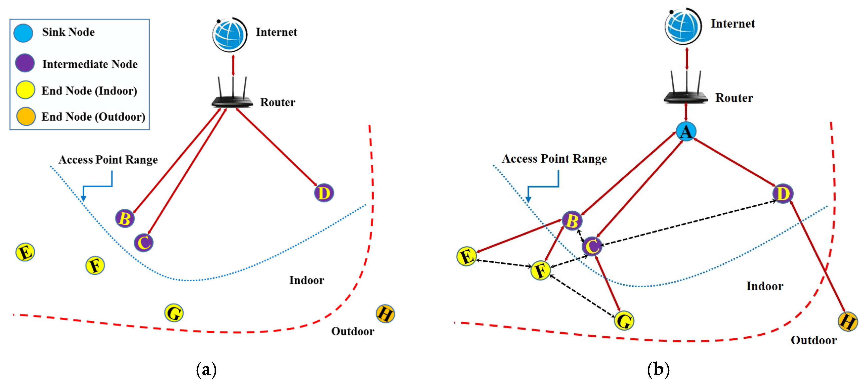
By using the ESP-MESH protocol, a huge number of Wi-Fi-enabled devices (e.g., ESP-32, ESP-8266, etc.) could be interconnected beneath a single wireless local-area network (WLAN) over a wide physical area. The main feature of this protocol is its self-healing and self-organizing property (the network could be built and sustained independently). The main disadvantages of the outmoded Wi-Fi network substructure are (1) the limited coverage area with the single access point shown in Figure 1a and (2) overloading (the capacity limitation of the access point).

The ESP-MESH overcomes the limitations of outdated infrastructure Wi-Fi networks in such a way that in ESP-MESH, the nodes are free to connect with their nearby nodes (there is no need to connect to a central node), shown in Figure 1b. Each node is commonly accountable for communicating with each other’s transmissions. This results in the ESP-MESH network covering a considerably better exposure area without requiring it to be in the range of the central node. Also, ESP-MESH seems to be less prone to congestion as there is no requirement for any node to connect the single central node.

The ESP-MESH network is a multi-hop network, which means that each node could transmit packets to another through one or more wireless hops in the network. Thus, each node in the network serves as a relay as well as transmitting its packets.

A network of ESP-MESH nodes may consist of three types: the sink node, the intermediate node, and the end node. The sink node interfaces directly with a conventional Wi-Fi router and relays packets between the nodes in the network and the external IP network. Only one sink node is present in an ESP-MESH network. Node A is the root node in Figure 1b.

An in-between node communicates, obtains data packets, and forwards data packets directed from its upstream and downstream connections (Nodes B, C, and D, are the intermediate nodes in Figure 2b). An end node could be able only to transmit or receive its packets. However, it cannot forward the data packets of other nodes (Nodes E, F, G, and H, are the end nodes in Figure 2b). sink/root node selection, layer formation, and limiting tree depth are the three steps of the ESP-MESH network-building process, as shown in Figure 2. The ESP-MESH is a self-healing network since it perceives and corrects for letdowns in network routing.

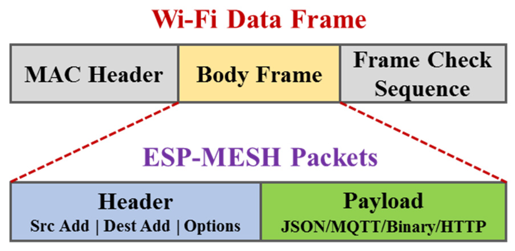
The following diagram shown in Figure 3 represents the arrangement of an ESP-MESH packet and its linkage with a Wi-Fi data frame. The header contains the media access control (MAC) addresses for both the transmitter and receiver nodes. The actual data are available in the payload of the MESH packet. The payload of an ESP-MESH packet comprises the definite application data and may contain either encoded data (MQTT, JSON, and HTTP) or raw binary data.

2.1. Selection of the Root/Sink and Intermediate Nodes

The sink node may be automatically set up or chosen by the administrator. The signal intensities of all idle nodes relative to the router determine the automatic selection of a sink node. Each idle node would send its addresses (MAC) and router RSSI values through Wi-Fi beacon packets. Then, every node concurrently scans for beacon packets from other idle nodes. If a node identifies a beacon packet with a greater router RSSI, it would initiate sending the frame’s information. The broadcast and scanning procedure would continue for a predetermined minimum number of iterations (10 iterations is the default setting), resulting in the propagation of the beacon packet with the greatest router RSSI across the network. Every node would verify its vote percentage (the count of votes or number of nodes taking part in the election) after all iterations to decide whether it becomes the sink node. If a node’s vote percentage exceeds a predefined threshold (90% is the default setting), the node becomes a sink node.

Figure 4 shows the construction of an ESP-MESH network when the sink node is selected automatically. The beacon frame with the strongest router RSSI is transmitted across the network after numerous iterations of broadcasting and scanning. Node A has the strongest router RSSI (−15 dB); as a result, its beacon frame is broadcast across the network. All nodes participate in the election vote for node A, providing it with a 100% vote share. Thus, node A becomes a sink node and establishes a connection with the router. Nodes B/C/D/H link to node A since they are the preferred intermediate nodes after node A is connected to the router. Nodes F and G link to node C, while node E connects to node B, concluding the network construction process.

Using the “esp_mesh_set_attempts()” function, the minimum number of election process iterations may be configured. Users must modify the number of iterations dependent on the number of network nodes (i.e., the more extensive the network, the greater the necessary number of scan iterations).

The threshold for the vote percentage may also be set using the “esp_mesh_set_vote_percentage()” function. Setting a low vote threshold percentage may result in two or more nodes becoming sink nodes in the same ESP-MESH network, forming several networks. If such is the case, the ESP-MESH provides internal capabilities to resolve the sink node disagreement autonomously. Multiple sink node networks would be merged into a single network with a single sink node. In addition, setting a small number of iterations and a low voltage threshold percentage might cause network instability owing to RSSI variations [19,20,21].

The administrator may also nominate the sink node, which would result in the specified sink node communicating directly with the router and bypassing the voting mechanism. Whenever a sink node is selected, all other nodes must forego the voting mechanism to avoid a sink node dispute.

Following the sink node’s connection to the router, the idle nodes in the vicinity of the root node would begin connecting to the sink node, creating the second layer of the network. Once joined, the second layer nodes become intermediate nodes, forming the third layer. Figure 2 shows that nodes B, C, and D are reachable from the sink node. As a result, nodes B, C, and D become intermediate since they establish upstream connections with the sink node. The connected nodes on the topmost layer of the network would immediately become terminal nodes to prevent the network from expanding over the maximum number of levels. This prevents a newer layer from emerging by preventing the unused nodes from communicating with the terminal node. Furthermore, if there is no other idle node that may serve as an intermediate node, the node would stay idle forever.

2.2. Network Management

The ESP-MESH is a self-healing wireless network because it detects and rectifies routing failures. The ESP-WIFI-MESH manages sink node failures as well as intermediate node failures.

2.2.1. Sink Node Failure

If the sink node breaks down, the nodes connected with it would promptly detect the failure of the sink node. The second layer nodes would initially attempt to reconnect with the sink node. Nonetheless, after numerous unsuccessful attempts, the second layer nodes would initiate a fresh round of sink node election. The second layer node with the highest router RSSI would be selected as the new sink node, while the other second layer nodes would establish an upstream link with the newly chosen sink node.

If the sink node and many descending layers subsequently failed (for example, the root node, second layer, and third layer), the shallowest layer that was still operational would initiate the root node election. Figure 5 demonstrates the self-healing mechanism after a root node failure. Sink node A would attempt to reconnect if it becomes disconnected. The second layer nodes initiate the voting process by transmitting their RSSIs after numerous unsuccessful attempts to rejoin. Node D’s router RSSI is the greatest. Node D is chosen as the sink node and starts to accept the downstream links. The other nodes on the second layer, B and C, establish upstream links with node D, restoring the network to regular operation.

2.2.2. Intermediate Node Failure

If an intermediate node fails, the detached end nodes would first try to reconnect with the intermediate node. After numerous unsuccessful efforts to rejoin, every end node would begin scanning for possible intermediate nodes. If there are more viable intermediate nodes, every end node would choose a new desired intermediate node and establish an upstream link. If there are no other suitable intermediate nodes for a given end node, it would stay idle forever.

Figure 6 depicts self-healing in response to a failure of an intermediate node. If intermediate node B fails, the surrounding nodes, E and F, would notice the failure and seek to reestablish communication with node B. After many unsuccessful reconnect attempts, nodes E and F begin to pick a new favorite intermediate node. Node E is out of range from all intermediary nodes and is thus currently inactive. Node F is within the reach of nodes C and G, although node C is chosen due to its lesser depth. After joining with node C, node F becomes an intermediary node, allowing node E to link. The connectivity is restored, but its routing is altered, and an additional layer is introduced.

2.2.3. Asynchronous Switching-on Reset

The sequence in which nodes the switch on may influence the formation of the ESP-MESH networks. If specific nodes within the network turn on asynchronously (i.e., delayed by a few minutes), the network’s final configuration may vary from the ideal scenario in which all nodes turn on synchronously. The following conditions would apply to nodes that are delayed when powering on:

Condition 1: If there is an existing sink node in the network, the delayed node would not try to vote in a new sink node, even if it had a greater RSSI. Instead, the delayed node would connect to a suitable intermediary node and join the network as any idle node would. If the delayed node is the assigned sink node, all other network nodes would remain inactive until it activates.

Condition 2: When a delayed node establishes an upstream link and becomes an intermediate node, it may also become the favored intermediate of the adjacent nodes. It would result in the neighboring nodes switching their upstream links to join the delayed node.

Condition 3: If an idle node has a specified intermediate node that is delayed when switching on, it would not try to create any upstream links in the lack of its specified intermediate node. The inactive node would stay inactive forever until its assigned intermediate node arrives.

Figure 7 depicts the impact of asynchronous power on network construction. Nodes A, C, E, F, G, and H are switched on simultaneously and start the sink node election procedure by transmitting their addresses (MAC) and router RSSIs. Node A is chosen as the sink node since its RSSI is the highest. As node A becomes the sink node, the other nodes start constructing upstream links with their selected parent intermediate, layer after layer. Nodes B and D are slow in switching on, although neither attempts to become the sink node, despite having a greater router RSSI (−10 dB) than node A. Instead, both delayed nodes establish upstream links with their selected root node, node A. Following the completion of the node joining, nodes B and D would each take on the role of an intermediate node.

If the network started up simultaneously, node D would have been the root since its router RSSI is the highest (−10 dB). To put it another way, the network architecture built under synchronous power on circumstances would look quite different from the one produced under asynchronous power on conditions.

2.2.4. Sink Node Switching

The ESP-MESH protocol does not switch the sink node automatically until the root node fails. The sink node would stay unaffected even if its router RSSI declines to the point of disconnection. Sink node switching is actively initiating a fresh election in which a node with a stronger router RSSI is chosen as the new sink node. This may be an effective strategy for adjusting to the deteriorating sink node performance. When the existing network requires a sink switch, the sink node must explicitly use the “esp_mesh waive_sink()” function to initiate a fresh election. At this time, the sink node would request that all other nodes in the network transmit and scan the beacon frames through a broadcast, after which it would stay networked. If another node wins more votes than the current sink node, the sink switching procedure would begin; otherwise, the sink node would remain unaltered.

The newly chosen sink node sends a switch request to the existing sink node, and the current sink node responds with an indication that it is prepared to switch. Upon receiving the answer, the newly chosen sink node would separate from its parent node and instantly establish an uplink connection to the router, becoming a new sink node in the network. The initial sink node would detach from the router while retaining all downlink connections and entering a state of inactivity. The preceding sink node would initiate a search for prospective parents and choose the desired parent.

Also, sink node switching must need an election and is thus only supported when a self-organized ESP-MESH network is in use. In other words, if a user-defined sink node is used, sink node switching cannot occur.

3. Time-Division Multiple-Access (TDMA) Scheduling Algorithms

The MESH network needs to guarantee that the data is correctly received regardless of the distance between the sensor node and the sink node. It is imperative that the intermediate nodes and sensor nodes coordinate the time window so that the intermediate node is in the receiving mode while the sensor node is transmitting data since sensors that are beyond the communication range of routers must locate an intermediate node to route their data.

Constantly opening the reception channel of the intermediary node is an easy solution to this coordination issue. However, an always-on receiving channel wastes energy. Hence, we adopt a TDMA scheduling algorithm (Algorithm 1) [22] to our MESH network (Figure 1b).

A setup step is required to construct the transmission schedule for the algorithm to function properly. The setup phase includes the following actions; hello, routing messages sent across sensor nodes, the transfer of necessary data to the sink node, the computation of the schedule, and the sensor nodes receiving the schedule via flooding.

The sensor node is then aware of all the other sensor nodes (neighbors) within its communication range and the next sensor node on its path toward the sink node. To determine the appropriate TDMA schedule, each sensor node in the MESH network (Figure 1b) transmits the above information to the root node, which uses Algorithm 1 outlined in the pseudo-code.

Algorithm 1 Pseudo-code used to define the TDMA schedule.
Line-1	Input: node-list Response: schedule
Line-2	do
Line-3	slot = new_Slot ();
Line-4	set-send-colsn = [];
Line-5	set-recv-colsn = [];
Line-6	while node-list: length > 0 do
Line-7	node = node-list [0];
Line-8	if (node.recv == 0 && (node: absent in set-send-colsn) && (node-dest: absent in set-recv-colsn)) then
Line-9	slot[node] = ‘SEND’;
Line-10	slot[node-dest] = ‘RECV’;
Line-11	set-send-colsn.include(node-dest-neighbors)
Line-12	set-send-colsn.include(node-dest)
Line-13	set-recv-colsn.include(node-neighbors)
Line-14	node-dest.recv--;
Line-15	node-list.eliminate (node);
Line-16	schedule: insert (slot)
Line-17	while slot: length > 0
Line-18	return schedule

As illustrated in

Table 1. Information about the sample network’s connectivity.

Node	Neighbors	Dest	Hops	Recv
A	B, C, D	ROUTER	0	3
B	A, C, E, F	A	1	2
C	A, B, G, F	A	1	1
D	A, C, H	A	1	1
E	B, F	B	2	0
F	B, C, E, F	B	2	0
G	C, F, H	C	2	0
H	D	D	2	0

Neighbors: The node’s one-hop neighbors. Dest: The routing protocol’s next-hop neighbor for the router. Hops: The variety of times a packet must be forwarded to a router. Recv: Listening slots. The receiving property ensures that the wake-up messages arrive in a TDMA frame.

, a “node-list” structure is produced for the network shown in Figure 1b. To calculate the TDMA schedule, Table 1 contains the following information: the neighbors of each node, the next hop destination for each node, the number of hops until the router, as well as the number of reception slots required before transmission begins.

The TDMA schedule is shown in

Table 2. The resulting TDMA schedule S indicates that the node sends in the specified timeslot, and R indicates that the node receives at the specified time slot.

Node	1	2	3	4	5
A			R	R	R
B	R	R	S
C		R		S
D		R			S
E		S
F	S
G		S
H		S

. R corresponds to a certain time slot during which the sensor node turns on its receiver, while S represents the sending time slot for every node. The following are descriptions of how Table 2 was generated using Table 1 and Algorithm 1.

Firstly, the node set is generated, including all the network’s nodes that have yet to be assigned a transmission slot. Next, the node set is ordered to boost the overall performance. Specifically, the nodes with high hops are positioned at the top so they may transmit in the first available slots, reducing the overall frame length. This is because the overall frame span would be at a minimum as long as the index number of the existing slot plus the value of the new node’s “hops” attribute. Furthermore, nodes with more neighbors are prioritized over nodes with fewer neighbors since these nodes are more likely to appear in the next collision list. A collision list is a collection of nodes that may create a collision if they broadcast in the same timeslot. The “set-send-colsn” list includes the nodes whereby a transmission would clash with an existing node in the timeslot. The “set-recv-colsn” list includes the nodes that would overhear a signal based on its timeslot. A potential broadcast toward such nodes could result in a collision, preventing the sender from joining the timeslot. Consequently, the following node list is constructed for the MESH network, seen in Figure 1b:

Node list = {F, G, E, H, B, C, D, A}.

Initially, the collision set contains no values. Following the preceding node list, we begin with node F. As per Table 1, the dest node of F is B, and the “Recv” term is zero. Thus, in Table 2, “S” and “R” are filled in slot one for nodes F and B, respectively. Node B and its neighbors are added to the “set-send-colsn” list, transforming it into {A, B, C, E, F}. The “set-recv-colsn” list is now populated with the neighbors of node F and becomes {B, C, E, G}. The “Recv” term of dest node B is lowered by one, resulting in a value of one.

Now, node G is chosen. In this instance, G’s dest node is C, and the “Recv” term equals zero. Then, we verify the availability of node G in the previous “set-send-colsn” list and node C in the prior “set-recv-colsn” list before determining which slot to use. Checking reveals that node C is included in the “set-recv-colsn” list; hence, “S” and “R” are populated in slot two against nodes G and C in Table 2. The “set-send-colsn” list is now {A, B, C, F, G} and “set-recv-colsn” is {C, F, H}. The “Recv” term of dest node C becomes zero.

The dest node for node E is B, and the “Recv” term is zero. Both nodes E and B are absent from the preceding “set-send-colsn” and “set-recv-colsn” lists; thus, slot two is populated with them. Table 2 is populated with “S” and “R” against nodes E and B. The “Recv” term of dest node B is decreased by one and becomes zero.

This method is continued until every sensor node has had the chance to transmit, at which point the node list is emptied. The first investigated node for each slot is always inserted due to the algorithm’s execution. Therefore, the procedure concludes when the planned slot has no nodes. Table 2 displays the resultant slot positions.

4. Design and Implementation of the (Air Pollution Monitoring) APM System

4.1. General Overview

Figure 1 shows the schematic illustration of the APM system, which consists of the access point (router), sink sensor node, intermediate sensor node, and end sensor node. All sensor nodes are placed inside the building at different locations for inside air quality monitoring except one; one of the sensor nodes is placed outside the building for outdoor air quality monitoring. The sensors associated with each sensing node monitor the air quality parameters inside and outside the building and transmit data to the root sensor node. The actual picture and the block diagram of the sensor node are shown in Figure 8 and Figure 9. All sensor nodes consist of a sensor module (with in-built Wi-Fi), a power module, and an MCU controller module.

4.2. Hardware

4.2.1. Sensor Selection

Table 3. Specifications of MQ gas sensors.

Sensor	Detects	Concentration	Operating Voltage	Power Consumption	Interface
MQ-135	Air quality (benzene, alcohol, NH3)	10 ppm–1000 ppm (C6H6) 10 ppm–300 ppm (NH3) 10 ppm–300 ppm (Alcohol)	5 V ± 0.1	750–900 mW	Analog
MQ-2	Methane, butane, LPG, smoke	300–10,000 ppm (combustible gas)
MQ-7	Carbon monoxide	20 ppm–2000 ppm (CO)

briefly describes gas sensors (MQ-135, MQ-2, and MQ7) [23] in terms of their applications, concentration ranges, operating voltages, power consumptions, and interfaces to the microcontroller unit. MQ series gas sensors are cheap and easy-to-find sensors with different models that allow us to detect different kinds of gas. It is a metal oxide semiconductor (MOS) type of gas sensor known as a chemi-resistor. The recognition is founded upon the modification of the resistance of the detection quantifiable when the gas originates during the interaction with the solid. Employing simple interface electronics (a resistance to voltage conversion), the concentrations of gas are easily sensed. The output voltage (in the analog form) provides the sensor with variations relative to the concentration of smoke or gas. Here, the gas concentration is proportional to the measured output voltage. MQ gas sensors work on 5 V DC. The output signal (in the analog form) from the MQ gas sensor is further fed to the high-precision comparator (LM393) to convert to a digital form. Also, the sensitivity of the sensor could be adjusted by using a tiny potentiometer which could be used to tune the concentration of the gas.

The parameters of the environmental sensor (BME280) and Laser PM2.5 Sensor (HM3301) are also summarized in

Table 4. Specifications of PM2.5 and BME280.

Laser PM2.5 Sensor (HM3301)
Particle Size	Resolution	Range	Operating Voltage	Power Consumption	Interface
2.5 µm, 5 µm, 10 µm	1 µg/m3	1~500 µg/m3	3.3 V/5 V	˂375 mW	I2C
BME 280
Parameter	Resolution	Range	Operating Voltage	Power Consumption	Interface
Temperature	0.01 °C	−40 °C to + 85 °C	1.71–3.6 V	6.12–12.96 µW	I2C
Humidity	0.008% RH	0 to 100 %RH
Pressure	0.18 Pa	300 to 100 hPa

. BME280 is a small and low-power sensor for measuring the relative humidity, barometric pressure, and ambient temperature produced from BOSCH, with an I²C protocol and a wide operating voltage range appropriate for various applications [24]. The Laser PM2.5 Sensor (HM3301) is a high-precision laser dust detection sensor that could be used for continuous and real-time dust detection in the air. The HM-3301 is based on the advanced Mie scattering theory [25]. The HM-3301 dust sensor is composed of the foremost components, such as an infrared (IR), the laser source, a fan, a photosensitive tube, a condensing mirror, an amplifier, and an interface electronics circuit.

Its stable output, ultra-low-power consumption, and little noise render it appropriate for intelligent air purifiers, air conditioners, and other air quality-related IoT projects.

4.2.2. Wi-Fi-Enabled MCU Module

As per the requirements of an indoor or outdoor sensor module (analog ports and the I2C interface) and wireless communication module, we selected an ESP32-DevKitC microcontroller. MQ gas sensors require an MCU, which has analog inputs, whereas BME280 and HM3301 need an I²C interface. The ESP32-DevKitC V4 board is a low-power, low-cost, Wi-Fi-enabled MCU produced by Espressif. This microcontroller offers 12-bit SAR ADC (up to eight channels), three UART, and advanced communication interfaces: up to two I2C and SPIs, etc. These features render the ESP32-DevKitC V4 board suitable for this proposed APM system.

4.2.3. Power Module

The main purpose of this module is to power the sensor nodes. Two types of supply voltage are required, 3.3 V for the BME280/HM3301 and 5 V for the MCU/MQ gas sensors. A power converter board (220–5 V, 3-A) which converts a 220 V AC supply to 5 V DC, was used to power the nodes. An ASM1117-3.3 IC was connected to the 5 V output and converted into a 3.3 V DC.

4.3. Software

To smoothly create an ESP-MESH network with Wi-Fi-enabled boards (e.g., ESP-32, ESP-8266, etc.), the PainlessMesh library was used [26]. By using the Painless MESH library, a programmer could focus on a MESH network without having to be concerned with how the MESH network is managed or structured. The flowchart of the complete software is shown in Figure 10.

Along with the Painless MESH library, other libraries were also used to interface the sensors with the ESP32. The Adafruit_Sensor, Adafruit_BME280, and Seeed_HM330X libraries were used to interface the temperature, humidity, PM2.5, gas sensors, etc.

In Painless Mesh, JSON objects were used for all the messaging to create and handle the JSON strings with the help of the Arduino_JSON library. After including the required libraries, MESH details, such as MESH_PREFIX, MESH_PASSWORD, and the MESH port, were included. Users could randomly choose the MESH_PREFIX and MESH_PASSWORD, provided that all the MESH network nodes had the same credentials. The value of the default MESH port was 5555.

Several functions were used in the Painless MESH library. The “get Readings” () function collected the readings of the sensor values, such as the PM 2.5, gas sensor, temperature, humidity, etc., and concatenated all the sensor values with a node number on a JSON variable called “JSON Readings”. The “send Message ()” function broadcasted the JSON string of the sensor values and node number (“get Readings ()” to all other nodes in the MESH network). Using the task “send message”, the function “sends Message ()” would be called every second as long as the program runs. Otherwise, several callback functions (received Callback (), new Connection Callback (), changed Connection Callback (), and node Time Adjusted Callback ()) would be called when some event on the MESH happens.

Finally, to keep the MESH running repeatedly, a functioning MESH update () was added to the loop ().

5. Results and Discussion

To measure the values of the different air quality parameters (temperature, humidity, PM2.5, etc.), data was taken (every 2 min) from node C (the indoor data) and node H (the outdoor data), as shown in Figure 11, Figure 12, Figure 13, Figure 14, Figure 15 and Figure 16. The parameters were continuously monitored for a duration of 72 min from 8 am to 09.12 am. All data were successfully monitored at root node A. Moreover, the sink node could be connected to the Wi-Fi-enabled router to send the data to the cloud.

To verify the effectiveness of the ESP-MESH network for air quality monitoring, we conducted several tests with real-world deployments.

5.1. Network Stability Test

To conduct the performance and network stability test, the configuration shown in Figure 1b was used. All seven nodes were placed in an open ground area (without any wall or barrier between the nodes). Each node in the MESH network was programmed to transmit one 64 Bytes data package per minute for five days.

The root node (which acts as a traffic monitoring receiver) recorded the data packages from all the nodes as the performance indicator. The stability, as well as the reliability of all data packet deliveries for each node, was evaluated using the rate of packet delivery (RPD):

$${\mathrm{RPD}}_{\mathrm{j}}=\frac{{\displaystyle \sum }\#{ \mathrm{Received}}_{\mathrm{j}}}{{\displaystyle \sum }\#{ \mathrm{Expected}}_{\mathrm{j}}}$$

where RPDj is the rate of packet delivery of the ‘jth’ node during five days. # Received is the number of packets at the center node, and # Expected is the number of packets that should be received.

$$\mathrm{Total}\_{\mathrm{RPD}}_{\mathrm{d}}=\frac{{{\displaystyle \sum }}_{\mathrm{d}}\# \mathrm{Received}}{{{\displaystyle \sum }}_{\mathrm{d}}\# \mathrm{Expected}}$$

where Total_RPDd is the total rate of packet delivery of all the nodes during the dth day.

The number of expected packets was estimated based on the particular node with a specific transmission interval (60 s). Instead of evaluating the parameters of a specific node, the Total_ RPDd provides an outline of the system stability of the time synchronization and time-division multiple-access (TDMA) routing.

The results of the RPDi and Total_RPDd for the five-day test are shown in Figure 17 and Figure 18. All the nodes show greater than 98% of RPD, and all the values of the Total_ RPDd are nearly 99%. Both results show that the network is stable and reliable. However, a significant network constraint may arise during the TDMA schedule’s flooding. Due to the simplicity of the architecture, one TDMA schedule table was flooded to each node in our present arrangement. Nonetheless, flooding the table necessitates the transmission of several packages over the network. This strategy could increase the setup phase overhead and impact the time synchronization. Once the synchronization is disrupted, a time slot mismatch would occur, resulting in either missing packages (a TX/RX window conflict) or package collisions (a TXs windows conflict).

In our future work, we would partition the table according to the routing route instead of sending the complete network table to every node simultaneously. Each multi-hop route in the network would obtain the required TDMA schedule only. This strategy would drastically minimize the setup phase overhead time without compromising the network’s performance.

5.2. Power Consumption

The power consumption depends on the contributing node’s location in the MESH network hierarchy and the network’s topology type. For every cycle, all the active nodes transmit a 64-byte data package, including the sensor readings.

As shown in Figure 19, all the nodes are associated with the ESP-MESH protocol. For each TDMA scheduling cycle, node E transmits a single package via the ESP-MESH to node B, and node B advances this package plus its package to node A via the same ESP-MESH network.

The current was measured using a True RMS meter from Fluke. Each sensor node (ESP32 + sensors) was powered with 5 V DC.

Table 5. Average current consumption of each node.

Sensor Nodes	Average Current Consumption (mA)
A	470.80
H	552.10
E, F, G	462.10
B, D, C	481.80

depicts the average current consumption of each node. The power consumption of different nodes was determined by the number of receive/transmit windows. It is to be noted that all the nodes consumed nearly 500 mA of current, which is due to the use of the air quality sensors (MQ-2, MQ-135, MQ-7, and HM3301). For low-power air quality sensors, the current consumption of the nodes would be low; in that case, the MESH network could have a very acceptable expected battery life across all the nodes.

5.3. Campus Deployment

For campus deployment, we used a college campus of a 100 m by 80 m area to place the sensor nodes (seven nodes) at different locations. All eight deployed nodes were continuously working for a duration of five days. A complete MESH network, shown in Figure 19, was established for the performance analysis of the campus-scale deployment. For the deployed network, the actual ESP-MESH link is represented by a solid line, whereas the dotted lines represent the available links (which are not being used). The furthest node (H) was placed 100 m away from the root node (A) and across more than four buildings and walls.

For the evaluation of the MESH network, a 64 Byte package was transmitted for five days at two-minute intervals, i.e., a total of 3600 (5 days × 24 h × 60 min/2 min) packages were anticipated to transmit from each node.

The effectiveness of the network was analyzed by evaluating the rate of packet delivery (RPD), package loss rate (PLR), and package fault rate (PFR) of all the active nodes. Similar to the RPD, the PFR depends on the number of faulty packages, and the PLR relies on the number of lost packages:

$${\mathrm{PFR}}_{\mathrm{j}}=\frac{{\displaystyle \sum }\#{ \mathrm{Fault}}_{\mathrm{j}}}{{\displaystyle \sum }\#{ \mathrm{Expected}}_{\mathrm{j}}}$$

$${\mathrm{PLR}}_{\mathrm{j}}=\frac{{\displaystyle \sum }\#{ \mathrm{Expected}}_{\mathrm{j}}-{\displaystyle \sum }\#{ \mathrm{Received}}_{\mathrm{j}}}{{\displaystyle \sum }\#{ \mathrm{Expected}}_{\mathrm{j}}}$$

Based on the received and expected packages for each node (seven nodes), an end-to-end RPD, PLR, and PFR are shown in Figure 20. From Figure 20a, it can be seen that the ESP-MESH network accomplishes more than 97% RPD, except for node H. Moreover, the PER and PLR (see Figure 20b,c) for each active node are under the limit (less than 1.8%) except for node H. Node H showed values of a higher PER and PLR (>1.8%); we suspect it might be due to its outdoor location. These results show that the ESP-MESH network offers a considerably good quality of service, mainly for medium-area networks [26,27,28].

5.4. Evaluation of the Performance

To confirm the effectiveness of the ESP-MESH network protocol, some important performance parameters were recorded. To measure the healing time after the sink node and intermediate node failure, we disconnected the power supply of a node (the sink and intermediate node) arbitrarily and measured the time spent. After many tests, several typical values were taken out. The experimental results are shown in

Table 6. Performance of the ESP-MESH protocol.

Performance Parameter	Time Spent
Network-building time	17.32 s
Healing time after the sink node failure	4.18 s
Healing time after the intermediate node failure	3.46 s

.

6. Conclusions

In the recent developments of wireless protocols (Zig-Bee, Wi-Fi, LoRa, etc.), the ESP-MESH networking protocol is low-cost, easy to implement, medium-range, and low-power option. This protocol does not require any internet connection to create a wireless network. Compared to LoRa, this protocol has a low range but is easy to implement. Devices used to establish the ESP-MESH network are very cheap in cost. In this work, we successfully established an ESP-MESH network that permits abundant sensor nodes spread over a large physical area to be consistent under a single WLAN for accurately measuring air quality and detecting air pollution events and sensors’ abnormal operations. First, we designed and developed system hardware, which contained a gateway, a base station, and sensors to collect indoor and outdoor air quality measurements. Then, the system software was intended to allow for data acquisition, processing, transmission, and energy conservation approaches for the complete system.

Moreover, a custom time-division multiple-access (TDMA) scheduling scheme for energy efficiency was applied to construct an appropriate transmission schedule that reduces the end-to-end transmission time from the sensor nodes to the router. To confirm the effectiveness of the network, data were taken from different air quality parameters (temperature, humidity, PM 2.5, gas concentrations, etc.) every 2 min from the indoor node and outdoor node and continuously monitored for a duration of 72 min from 8 am to 09.12 am. The network-building time, healing time after sink node failure, and intermediate node failure were recorded as 17.32 s, 4.18 s, and 3.46 s, respectively. Additionally, the experiment of the sensor accuracy measurement in real physical activity was provided. Finally, the performances of the communication interfaces were assessed, including the package loss rate (PLR), package fault rate (PFR), and rate of packet delivery (RPD). The results showed that the ESP-MESH network accomplished more than 97% of most nodes’ RPDs. Also, the PMR and PER for each active node were under the limit (less than 1.8%).