Spatial-Temporal Evolution and Convergence Characteristics of Agricultural Eco-Efficiency in China from a Low-Carbon Perspective

Abstract

While agriculture plays an essential role in food security, it is also one of the largest emitters of carbon emissions. China’s carbon neutrality and carbon peaking goals mean that China’s agriculture is also going through a low-carbon transition. To analyze the spatiotemporal heterogeneity and convergence of China’s agricultural eco-efficiency (AEE), this study used a combined super-efficient slacks-based measure (SBM), global Malmquist–Luenberger index (GML), kernel density estimation, Moran index, and convergence model on panel data from 2005 to 2020 and from 31 Chinese provinces. An innovative eco-efficiency index evaluation system was constructed from a low-carbon perspective that integrated agricultural carbon sinks and carbon emissions. The results revealed that the average AEE movement was U-shaped, but there were significant differences across regions and periods. The AEE demonstrated a gradual decreasing pattern of “northeast > eastern > western > central”, a declining trend during 2005–2010 and increasing trends during 2011–2020. The main reason for AEE growth was technological progress; however, technical efficiency only played a role in several provinces. The AEE in Chinese provinces was also found to have spatial autocorrelation characteristics dominated by high-high, low-low, and high-low clustering. A “catching-up effect” existed in the lagging AEE regions. Therefore, it is recommended to promote the integration of regional strategies and low-carbon development, build a low-carbon technology support system, and construct a national agricultural carbon trading center to facilitate agricultural low-carbon transformation.

1. Introduction

Climate change has become a common global concern and has accelerated the global move to green, low-carbon production and lifestyles. Although industry has been recognized as the primary source of carbon emissions, agriculture is also a relatively large contributor to global carbon emissions growth [1], with agricultural food production emissions increasing by 17% over the past 30 years. The global food system now accounts for more than one-third of all global anthropogenic greenhouse gas emissions [2]. The IPCC’s Climate Change and Land special report identified agriculture and deforestation as critical drivers of climate change, with rice, farming, and nitrogen fertilizer significantly contributing to GHG emissions [3]. Climate change and increased extreme weather events have seriously impacted agricultural development [4], which in turn has threatened both food security and the terrestrial environment.

As a large developing agricultural country, China’s agricultural development pattern of “high input, high output, and high emissions” [5,6] has resulted in severe environmental pollution. In 2019, the Ministry of Agriculture and Rural Affairs reported that the average arable land grade was only 4.76/10, with 31.24% of arable land being below grade 3 [7]. The lack of arable land per capita and the uneven land quality has resulted in an overuse of chemical fertilizers and pesticides [8]. In 2021, as for China’s three major crops (rice, corn, and wheat), the total chemical fertilizer utilization rate was 40.2% and the total pesticide utilization rate was 40.6% [9]. While China ranks first in the world for fertilizer and pesticide use, its utilization rate is 10 to 20 percentage points lower than in developed countries. The use of fertilizers, pesticides, and fuel causes both agricultural nonpoint source pollution and carbon emissions, which offsets soil carbon sequestration [10]. China’s agricultural activities account for about 15% of national greenhouse gas emissions. At the same time, agriculture has both carbon reduction and carbon sequestration functions [1,11], which means that agriculture could significantly assist in meeting China’s dual carbon goals. Therefore, China has included agricultural carbon emissions reduction as one of the key actions needed to slow climate change. For example, the Ministry of Agriculture and Rural Development and four other departments jointly issued China’s first special green agricultural development plan, the 14th Five-Year Plan for National Green Agricultural Development [12].

As China moves to a low-carbon, sustainable eco-environment, accurate spatial-temporal AEE evolution evaluations are needed to ensure policymakers have the knowledge to develop appropriate agricultural carbon reduction policies. However, AEE studies have tended to focus more on the negative externalities caused by agricultural production. Many studies have constructed evaluation index systems that have taken agricultural carbon emissions or nonpoint source pollution as undesirable output [5,13,14,15,16,17], with only a few efficiency assessment studies considering positive agricultural production externalities other than economic output [18,19] and very few focusing on the value of carbon sinks. However, indicator systems that only consider negative environmental externalities reduce the comprehensiveness and accuracy of AEE assessments [1]. SBM has been widely used in AEE evaluation studies [5,15,19,20,21]; however, although a GML index based on an SBM directional distance function can effectively achieve global production frontier comparability and decompose the reasons for the AEE changes [22,23], there have been few studies that have combined SBM with GML and applied it to AEE assessments.

Given the limitations of existing research, this study attempted to innovate and extend these studies by making the following contributions. First, many previous studies have taken economic output as the only desirable output and have ignored agriculture’s environmental and ecological value [19,24,25]. Therefore, to present a more comprehensive assessment of AEE from a low-carbon perspective, this paper innovatively considered economic benefits and the carbon-sink values as expected output and agricultural carbon emissions as the undesirable output. Second, to compensate for time series incomparability, a nonradial, non-oriented, global super-efficient SBM model containing undesirable outputs was employed that constructed the production frontiers in all periods. Further, because GML has better continuity than the traditional ML index and can be directly projected to period one or backward to period T, the GML index and the super-efficient SBM were combined to examine the dynamic evolution and specific reasons for the efficiency changes [26,27]. Therefore, to provide a reference for sustainable, low-carbon agricultural development in China, this article assessed China’s low-carbon AEE spatial-temporal evolution and convergence characteristics using multi-dimensional analyses.

The remainder of this article is organized as follows: Section 2 reviews the literature, Section 3 details the research methods, Section 4 presents and discusses the empirical results, and Section 5 gives the conclusions and policy recommendations.

2. Literature Review

AEE, which was first defined in 1990 [28], is a specific eco-efficiency application for the agricultural sector. Eco-efficiency is defined as the ratio of increased economic value to inputs with environmental impact. In 1992, the Business Council for Sustainable Development (WBCSD) identified eco-efficiency as the provision of reasonably priced goods and services that meet the needs of high-quality human life while reducing the environmental impacts to a level consistent with the Earth’s carrying capacity. Subsequently, the Organization for Economic Cooperation and Development (OECD) and the European Environment Agency (EEA) further promoted the eco-efficiency concept by introducing several indicator assessment systems that have since been widely used [5]. Eco-efficiency is not only a simple assessment tool but also a useful instrument for the development of national and regional strategies [29]. With the sustainable use of agricultural resources at the core, AEE assessments seek to improve agricultural production efficiency, reduce resource inputs, and lower waste [19]. As an important criterion for agricultural sustainability [30], the AEE integrates agricultural economic and environmental benefits.

Various evaluation methods have been developed to assess eco-efficiency, such as the ratio method, life cycle assessment (LCA), and modeling [30]. The ratio method, and most typically the formula proposed by the WBSCD [31], takes a particular type of environmental pollution or resource consumption as the denominator and economic output as the numerator. The indicator approach focuses on economic outputs and ignores inputs; however, inputs are the deep-seated cause of environmental pollution [1] and affect agricultural productivity [4]. Thus, the indicator approach does not provide an accurate assessment. LCA examines the environmental impacts of products or services at each life cycle stage [32]; nevertheless, its accounting boundary delineation is subjective, and the data collection and processing costs are high [30]. Modeling methods can deal with multiple inputs and outputs, and the respective weights are allocated based on statistical data characteristics to derive a composite value. Two main modeling approaches, data envelopment analysis (DEA) and stochastic frontier analysis (SFA), have been commonly applied to eco-efficiency calculations. SFA is a parametric approach that allows for the estimation of technical efficiency to be controlled by estimating the production functions for individual production processes; therefore, SFA is more accurate than DEA because it fully considers the role of random error terms in individual efficiencies [33,34]. However, SFA is more suitable for situations with multiple inputs and single outputs or large samples [24,35], whereas DEA does not require a specific production function form to be set and can measure the relative efficiency of the same type of decision-making unit (DMU) in a multiple-input and output framework [36]. There is also no need to process the data to eliminate dimensionality before building the model, which makes DEA highly flexible [15,17]. Consequently, DEA has been widely used for efficiency studies at national [13,34], regional [6,37,38,39], and organizational levels, such as farms or companies [17,40,41].

The main traditional DEA models are the CCR model and the BCC model, adding the constraints of convex sets to the CCR model [42]. The efficiencies obtained from the CCR and BCC models are referred to as technical efficiency and pure technical efficiency. Two main drawbacks to these basic DEA models exist. The first is that radial DEA models do not consider slack variables in their inputs or outputs, which could lead to overestimation. The second drawback is that negative externalities (undesirable outputs) are not considered [5]. To overcome these shortcomings, Tone combined a directional distance function (DDF) and the Super-SBM model [43] to construct the Un_Super_SBM model, which was nonradial, non-oriented, and considered undesirable outputs [44]. The model involves both radial and nonradial redundancies, which means it fully considers the input and output improvement spaces, with the efficiency reducing as the slack variables rise. Given the advantages of the Un_Super_SBM model, many environmental economics studies have used this method to measure energy efficiency [14,45], urban eco-efficiency [27,46], AEE [20], and tourism eco-efficiency [47].

However, the efficiency values for different benchmarks are not comparable or circular when using panel data [48], which means that DEA models are unable to analyze eco-efficiency changes over time [49,50]. Therefore, the traditional DEA-Malmquist index needs to be improved to reflect dynamic eco-efficiency evolutions. The global Malmquist productivity index (GM) was proposed by constructing a production technology set comprising all-period DMU data as the common production frontier [51]. Oh then combined the GM and DDF to develop the global Malmquist–Luenberger productivity (GML) index [52]. Therefore, GML and SBM methods have been used to assess energy efficiency [53], comprehensive eco-efficiency [48], and total factor productivity growth [54,55].

Many empirical studies from different perspectives have been conducted to explore evolutionary characteristics of AEE in China. Since its reform and opening up, Chinese AEE has had significant stage characteristics: free development, reform promotion, market regulation, and policy incentives [5]. Using agricultural development and rural economic development as the first and second stages in determining the overall rural development efficiency, Ref. [16] concluded that China’s AEE was not high but the overall trend was favorable and showed growth. As the AEE closely correlates with economic income, the EKC curve for AEE in the Chinese scenario has been verified [8,19], and a spatial autocorrelation of AEE has also been found [15]. Provinces with high AEE were found to have positive spillover effects, while provinces with low AEE had negative spillover effects [20]. Sustainable agricultural development requires an effective trade-off between agricultural production and urbanization [56] and the promotion of agricultural transformation through agricultural technology research and development [8].

3. Research Methods and Data

3.1. Area and Data

This paper used the agricultural input-output data of 31 provinces in China from 2005 to 2020 as samples, excluding Hong Kong, Taiwan, and Macao. Four geographic regional unit classifications were applied according to those put forward by the Chinese National Bureau of Statistics [57]: eastern, central, western, and northeast (

Table 1. China’s four major regional classifications based on administrative provinces.

Regions	Provinces
Northeast region (N)	Liaoning, Jilin, Heilongjiang
Eastern region (E)	Beijing, Tianjin, Hebei, Shanghai, Jiangsu, Zhejiang, Fujian, Shandong, Guangdong, Hainan
Central region (C)	Shanxi, Anhui, Jiangxi, Henan, Hubei, Hunan
Western region (W)	Inner Mongolia, Guangxi, Chongqing, Sichuan, Guizhou, Yunnan, Tibet, Shaanxi, Gansu, Qinghai, Ningxia, Xinjiang

).

The data for each province were obtained from the official website of the National Bureau of Statistics (http://www.stats.gov.cn) (accessed on 2 November 2022), the China Agriculture and Forestry Statistical Yearbooks, and the statistical yearbooks from each province; the map data were collected from the national 1:1 million basic geographic databases of the National Geographic Information Center database (www.webmap.cn) (accessed on 2 November 2022). Missing values were first examined in the statistical yearbooks and communiques published by local governments, and if the data could not be accessed, they were completed using interpolation.

3.2. Index Construction

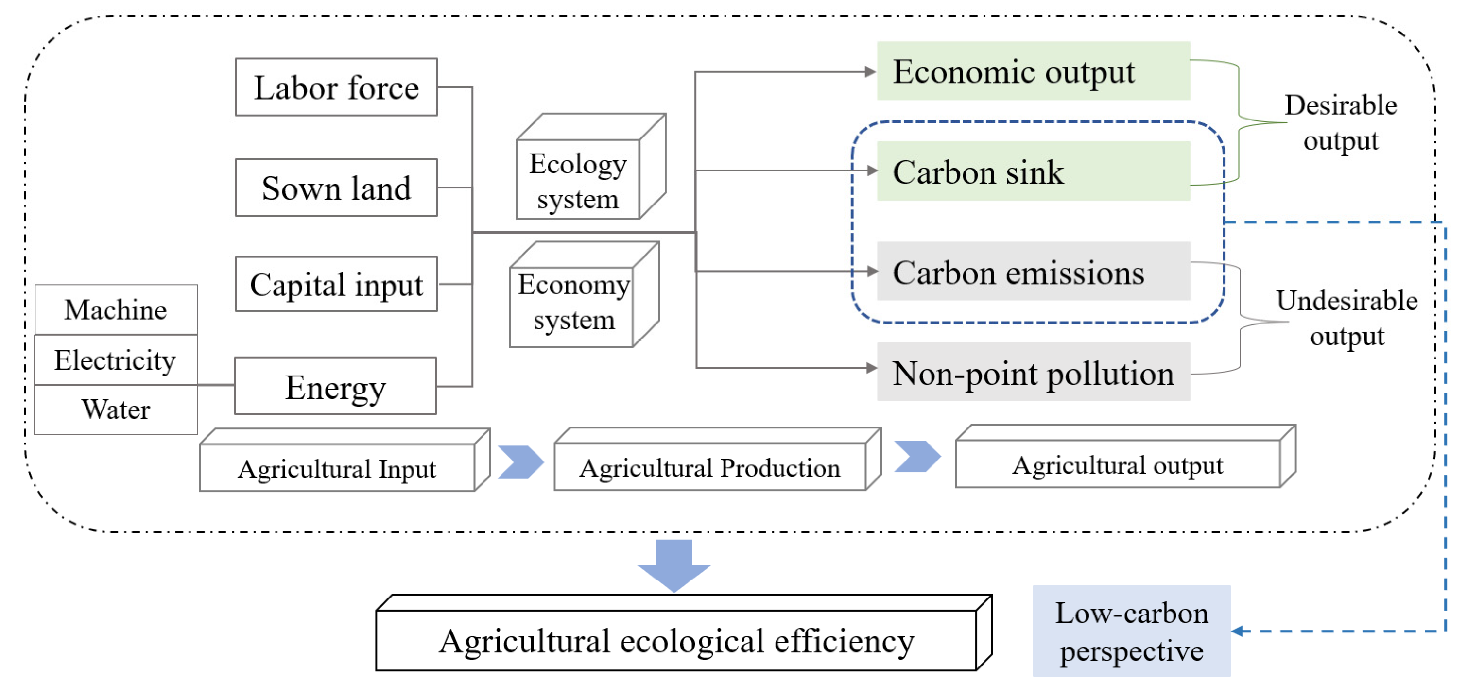
Based on previous studies [8,13,19,34], the research object was set as agriculture (plantation) in the primary sector and the indicator system (

Table 2. Descriptions of the agricultural eco-efficiency evaluation index system.

Primary Indexes	Sub-Indexes	Specific Variables	Indicator Description
Input indicators	Labor input	Labor force (10K people)	the labor force in the primary industry multiplied by the percentage of agricultural output in the primary industry
	Land input	Total crops sown area (thousand ha)	Actual cultivated area in agriculture
	Capital input	Fiscal expenditure for agriculture (10K CNY)	Agriculture, forestry, and water affairs expenses
	Energy consumption	Total power of agricultural machinery (10K KWH)	Diesel engines, gasoline engines, electric motors, and other mechanical power
		Rural electricity consumption (100 million KWH)	Electricity consumption in rural areas
		Effective irrigation area (thousand ha)	Using irrigated area as a proxy for water use
Output indicators	Desirable output	Gross agricultural output value (100 million CNY)	Economic gains of agriculture
		Agricultural carbon sink value (10K ton)	Ecological value of agriculture
	Undesirable output	Agricultural carbon emissions (10K ton)	Emissions from different carbon sources such as agricultural materials, rice, and irrigation
		Agricultural nonpoint source pollution (10K ton)	The use of three major agricultural materials such as fertilizers, pesticides, and films

) was established as shown in Figure 1. According to the rule of thumb outlined in [58], the number of indicators satisfied the requirement that the sum of DMUs was more than three times the total number of input and output variables.

3.2.1. Input Indicators

The production factors essential to agricultural activities, labor, land, capital, and energy, were selected as the inputs. The number of primary industry employees was converted based on the share of agricultural output in the primary industry. The agricultural price index was used to adjust to the 2005 price benchmark for the capital input, and the effective irrigated area was used to represent agricultural water consumption.

3.2.2. Desired Outputs

The total agricultural economic output and carbon sink sequestration values were used as the desired outputs. The agricultural price index was used to adjust data to the 2005 base to eliminate any price change effect on the total agricultural economic output. Meanwhile, drawing on [1], the agricultural carbon sink sequestration value was determined as follows:

$$C={{\displaystyle \sum }}_i{C}_i=\frac{{{\displaystyle \sum }}_i{C}_a{Y}_i\left(1-m\right)}{H{I}_i}$$

(1)

where $C$ was the carbon absorption of the crops (carbon sink), $C_i$ was the carbon absorption of i crop, $C_a$, m, and $H{I}_i$ were the carbon absorption rate (%), moisture content (%), and economic coefficient of the crop (%), respectively (see

Table A1. Economic coefficient, carbon absorption rate, and moisture content of crops in China [68] (Unit: %).

Crops	Economic Coefficient (Hi)	Carbon Absorption Rate (Cf)	Moisture Content (Wi)
Rice	45	41	12
Wheat	40	49	12
Corn	40	47	13
Beans	34	45	13
Potato	70	42	70
Cotton	10	45	8
Canola	25	45	10
Peanut	43	45	10
Sugarcane	50	45	50
Beets	70	41	75
Tobacco	55	45	80
Vegetable	60	45	90
Melon	70	90	45

), and $Y_i$ was the total economic crop yield.

3.2.3. Undesirable Outputs

The typical manifestation of agricultural pollution is nonpoint source pollution, which is mainly caused by three aspects: the loss of fertilizer nitrogen and phosphorus, the ineffective use of pesticides, and the residue of agricultural film [15]. Fertilizer nitrogen loss is the sum of the nitrogen content of the compound fertilizer and the nitrogen fertilizer amount multiplied by the nitrogen loss factor. Fertilizer phosphorus loss is the total amount of the phosphorus content of the compound fertilizer and the phosphorus fertilizer amount multiplied by the phosphorus loss coefficient. The amount of pesticide ineffective utilization is calculated by multiplying the amount of pesticide used and the pesticide ineffective utilization coefficient. The amount of film residue is measured as the amount of film used multiplied by the film residue coefficient. At the actual accounting level, the coefficients were determined by referring to [15,16] and the relevant data published by the National Bureau of Statistics of China. Three empirical indicators, “fertilizer × 0.65, pesticide × 0.5, and agricultural films × 0.1”, were adopted, meanwhile they were combined into a comprehensive indicator of “agricultural nonpoint source pollution” by the entropy value method [59].

The carbon source factors identified in this paper were divided into three main categories, as follows: (1) agricultural materials and, specifically, the carbon emissions resulting from fertilizer, pesticide, agricultural film, and diesel fuel use; (2) agricultural irrigation, which was related to power use, the thermal power generation for which has indirect carbon emissions; therefore, the thermal power coefficient was multiplied by $25\mathrm{kg}/{\mathrm{hm}}^2$ [60], and the thermal power coefficients for each province and year were calculated based on the 2005 to 2020 China Yearbook statistics as the thermal power generation ratio to total power generation; and (3) rice cultivation methane emissions, which were based on the rice growing areas each year and the median of the rice growing cycle of 130 days [61]. As the research object was agriculture in a narrow sense, the carbon emissions from ruminant farming were not considered.

$$C=\sum C_i=\sum M_i\times {\delta }_i$$

(2)

where C and $C_i$(the subscript i indicated the type of carbon source) denoted the total agricultural carbon emissions and the carbon emissions from each carbon source.$M_i\mathrm{and}{\delta }_i$ referred to the actual amount of each carbon source and its corresponding carbon emission coefficient (see

Table A2. Agricultural carbon emission source, coefficient, and reference sources.

Category	Carbon Emission Source	Coefficient	References
Materials	Agricultural fertilizer	0.8956 kg C/kg	Oak Ridge National Laboratory of the United States
	Pesticides	4.9341 kg C/kg
	Agricultural diesel	0.5927 kg C/kg	IPCC United Nations Intergovernmental Committee of Experts on Climate Change
	Agricultural plastic film	5.1800 kg C/kg	Institute of Agricultural Resources and Ecological Environment of Nanjing Agricultural University
Irrigation	Agricultural irrigation	25.0000 kg C/hm2	[69]
Rice	Rice farming	3.1360 g C/(m2-day)	[70,71,72]

).

3.3. Model Specification

3.3.1. Super-Efficient SBM Model Based on the Undesirable Output

Drawing on the Un_Super_SBM model [44], a production possibility set was constructed in which each province was treated as an independent DMU, and the optimal realization production boundaries for all provinces for each year were set. In reference to [62], suppose that at t = 1, 2,..., T period, each province k = 1, 2,..., K uses input vectors, “good” output vectors, and “bad” output vectors, that is, $x^{tk},y^{tk},$ and $b^{tk}.$ x denotes the N kinds of inputs for each DMU and x = ($x_1$,..., $x_n$) ∈ $R_N^{*}$, y represents the M kinds of desired outputs and y = ($y_1$,..., $y_m$) ∈ $R_M^{*}$, and b denotes I kinds of undesirable outputs and b = ($b_1$,..., $b_i$) ∈ $R_I^{*}$. As such, ($x_k^t,y_k^t,b_k^t$) and ($x_{k^{\prime }n}^t,y_{k^{\prime }m}^t,b_{k^{\prime }i}^t$) were the input-output data for period t in region k and $k^{\prime }$. The production possibility set for each province for the current period was obtained.

$$P^t\left(x^t\right)=\left\{\left(y^t,b^t\right):{{\displaystyle \sum }}_{k=1}^K{z}_k^t{y}_{km}^t\ge y_{km}^t,\forall m;{{\displaystyle \sum }}_{k=1}^K{z}_k^t{b}_{ki}^t=b_{ki}^t,\forall i;{{\displaystyle \sum }}_{k=1}^K{z}_k^t{x}_{kn}^t\le x_{kn}^t,\forall n;{{\displaystyle \sum }}_{k=1}^K{z}_k^t=1,z_k^t\ge 0,\forall k\right\}$$

(3)

where $z_k^t$ was the weight of each cross-sectional observation. If $\sum z_k^t$ = 1 and $z_k^t\ge 0,$ the production technology was viewed as variable returns to scale (VRS), and if $z_k^t\ge 0,\mathrm{the}\mathrm{production}\mathrm{technology}\mathrm{was}\mathrm{viewed}\mathrm{as}$ returns to scale (CRS). The current production possibility set $P^t\left(x^t\right)$ was replaced with the global production possibility set $P^G\left(x\right)$, which demonstrated that $P^G\left(x\right)=P^1\left(x^1\right)\cup P^2\left(x^2\right)\cup P^3\left(x^3\right)\dots P^T\left(x^T\right)$. Using the DEA method, Equation (4) was obtained.

$$\begin{array}{c}{P}^G\left(x\right)=\{\left(y^t,b^t\right):{{\displaystyle \sum }}_{t=1}^T{{\displaystyle \sum }}_{k=1}^K{z}_k^t{y}_{km}^t\ge y_{km}^t,\forall m;{{\displaystyle \sum }}_{t=1}^T{{\displaystyle \sum }}_{k=1}^K{z}_k^t{b}_{ki}^t=b_{ki}^t,\forall i;{{\displaystyle \sum }}_{t=1}^T{{\displaystyle \sum }}_{k=1}^K{z}_k^t{x}_{kn}^t\le x_{kn}^t,\\ \forall n;{{\displaystyle \sum }}_{k=1}^K{z}_k^t=1,z_k^t\ge 0,\forall k\}\end{array}$$

(4)

The following equation is the definition of the global Un_Super_SBM model:

$$\rho =min\rho =min\frac{1+(\frac{1}{N}{{\displaystyle \sum }}_{n=1}^N{S}_n^x/x_{k^{\prime }n}^t)}{1-\frac{1}{M+I}[{{\displaystyle \sum }}_{m=1}^M{S}_m^y/y_{k^{\prime }m}^t+{{\displaystyle \sum }}_{i=1}^I{S}_i^b/b_{k^{\prime }i}^t]}$$

$$s.t.x_{k^{\prime }n}^t\ge {{\displaystyle \sum }}_{t=1}^T{{\displaystyle \sum }}_{k=1}^K{z}_k^t{x}_{kn}^t-S_n^x,\forall n$$

$$y_{k^{\prime }m}^t\le {{\displaystyle \sum }}_{t=1}^T{{\displaystyle \sum }}_{k=1}^K{z}_k^t{y}_{km}^t-S_m^y,\forall m;$$

$$b_{k^{\prime }i}^t\ge {{\displaystyle \sum }}_{t=1}^T{{\displaystyle \sum }}_{k=1}^K{z}_k^t{b}_{ki}^t+S_i^b,\forall i;$$

$${{\displaystyle \sum }}_{k=1}^K{z}_k^t=1,z_k^t\ge 0,\forall k;$$

$$S_n^x\ge 0,\forall n$$

$$S_m^y\ge 0,\forall m$$

(5)

where $\rho \mathrm{denotes}\mathrm{the}AE{E}_{i,t}.S_n^x,$ $S_m^y,$ and $S_k^b$ were the slack vectors for the inputs and outputs that reached the efficiency frontier, and indicated the excessive inputs, the insufficient “good” outputs, and the excessive “bad” outputs, respectively.

3.3.2. Global Malmquist–Luenberger Productivity Index (GML)

Fukuyama and Weber’s method [63] determined the SBM directional distance function to be as follows:

$${\overrightarrow{S}}_v^G\left(x^{t{k}^{\prime }},y^{t{k}^{\prime }},b^{t{k}^{\prime }},g^x,g^y,g^z\right)=\frac{1}{N+M+I}\max \left({{\displaystyle \sum }}_{n=1}^N\frac{S_n^x}{g_n^x}+{{\displaystyle \sum }}_{m=1}^M\frac{S_m^y}{g_m^y}+{{\displaystyle \sum }}_{i=1}^I\frac{S_i^b}{g_i^b}\right)$$

$$s.t.{{\displaystyle \sum }}_{t=1}^T{{\displaystyle \sum }}_{k=1}^K{z}_k^t{x}_{kn}^t+S_n^x=x_{k^{\prime }n}^t,\forall n;$$

$${{\displaystyle \sum }}_{t=1}^T{{\displaystyle \sum }}_{k=1}^K{z}_k^t{y}_{km}^t-S_m^y=y_{k^{\prime }m}^t,\forall m;$$

$${{\displaystyle \sum }}_{t=1}^T{{\displaystyle \sum }}_{k=1}^K{z}_k^t{b}_{ki}^t+S_i^b=b_{k^{\prime }i}^t,\forall i;$$

$${{\displaystyle \sum }}_{k=1}^K{z}_k^t=1,z_k^t\ge 0,\forall k;$$

$$S_n^x\ge 0,\forall n;$$

$$S_m^y\ge 0,\forall m;$$

$$S_i^b\ge 0,\forall i;$$

(6)

where ${\overrightarrow{S}}_v^G\left(x^t,y^t,b^t,g^x,g^y,g^b\right)$ represented the global SBM directional distance functions and the current period DDF ${\overrightarrow{S}}_v^t\left(x^t,y^t,b^t,g^x,g^y,g^b\right)$ can be obtained by removing the time factor from the constraint. $g^x,g^y,\mathrm{and}{g}^b$ were the directional vectors that respectively indicated a decrease in inputs, a growth in “good” outputs, and a decrease in “bad” outputs.

The GML index shows the dynamic efficiency changes. The GML index can be decomposed into a technical efficiency change index (EC), which indicated the management system and resource allocation improvements, and a technological progress index (PBC), which indicated the production process and manufacturing skill improvements. In this way, the reasons for the eco-efficiency changes could be better explained [14]. The GML index and its decomposition were as follows:

$${\mathrm{GML}}_t^{t+1}=\frac{1+{\overrightarrow{S}}_v^G\left(x^t,y^t,b^t,g^x,g^y,g^b\right)}{1+{\overrightarrow{S}}_v^G\left(x^{t+1},y^{t+1},b^{t+1},g^x,g^y,g^b\right)}={\mathrm{EC}}_t^{t+1}\times {\mathrm{PBC}}_t^{t+1}$$

$${\mathrm{EC}}_t^{t+1}=\frac{1+{\overrightarrow{S}}_v^t\left(x^t,y^t,b^t,g^x,g^y,g^b\right)}{1+{\overrightarrow{S}}_v^{t+1}\left(x^{t+1},y^{t+1},b^{t+1},g^x,g^y,g^b\right)}$$

$${\mathrm{PBC}}_t^{t+1}=\frac{\frac{\left[1+{\overrightarrow{S}}_v^G\left(x^t,y^t,b^t,g^x,g^y,g^b\right)\right]}{\left[1+{\overrightarrow{S}}_v^t\left(x^t,y^t,b^t,g^x,g^y,g^b\right)\right]}}{\frac{\left[1+{\overrightarrow{S}}_v^G\left(x^{t+1},y^{t+1},b^{t+1},g^x,g^y,g^b\right)\right]}{\left[1+{\overrightarrow{S}}_v^{t+1}\left(x^{t+1},y^{t+1},b^{t+1},g^x,g^y,g^b\right)\right]}}$$

(7)

The GML index indicated the change in the t + 1 period relative to period t. If the index was greater than 1, the GML had increased; if the index was less than 1, the GML had decreased; if the index was equal to 1, the GML was considered to be in a stable state. This also applied to the EC and PBC indices.

3.3.3. Kernel Density Estimation Method

Kernel density estimation analysis is an important tool for studying spatially unbalanced distributions and can also portray an object’s evolutionary trends and patterns by comparing the distribution curve position, shape, extension, and polarization degrees in different periods [20]. The Gaussian kernel function used in previous studies was chosen to determine the AEE’s dynamic evolutionary trends in China from 2005 to 2020, for which the following equation was used:

$$f\left(x\right)=\frac{1}{Nh}{{\displaystyle \sum }}_{i=1}^{N}K\left(\frac{x_i-\overline{x}}{h}\right)$$

$$K\left(x\right)=\frac{1}{\sqrt{2\pi }}\exp \left(-\frac{{\mathrm{x}}^2}{2}\right)$$

(8)

where $f\left(x\right)$ was the kernel density function, $K\left(x\right)$ was the kernel function, N denoted the number of observations, $x_i$ stood for the independently and identically distributed observations, $\overline{x}$ was the mean value, and h was the bandwidth.

3.3.4. Spatial Autocorrelation Analysis

Spatial autocorrelation reflects the correlations between the spatial unit attribute value and the same attribute on a neighboring unit [4] and includes a global spatial autocorrelation and a local spatial autocorrelation [64], which were respectively expressed using the global Moran index ($I$) and the local Moran index ($I_i$).

$$I=\frac{n}{{{\displaystyle \sum }}_{i=1}^n{\left(x_i-\overline{x}\right)}^2}\times \frac{{{\displaystyle \sum }}_{i=1}^n{{\displaystyle \sum }}_{j=1}^n{w}_{ij}\left(x_i-\overline{x}\right)\left(x_j-\overline{x}\right)}{{{\displaystyle \sum }}_{i=1}^n{{\displaystyle \sum }}_{j=1}^n{w}_{ij}}$$

(9)

$$I_i=\frac{\left(n-1\right)\left(x_i-\overline{x}\right){{\displaystyle \sum }}_{j=1,j\ne i}^n{w}_{ij}\left(x_j-\overline{x}\right)}{{{\displaystyle \sum }}_{j=1,j\ne i}^n{\left(x_j-\overline{x}\right)}^2}$$

(10)

In Equations (9) and (10), n was the number of spatial units, $x_i$ and $x_j$ were the respective attribute values for unit i and unit j, and $w_{ij}$ was the spatial weight matrix. The matrix used in this paper was the inverse distance weight matrix.

3.3.5. Convergence Analysis

The equations for the absolute $\mathsf{\beta }$ convergence (Equation (11)) and the conditional $\mathsf{\beta }$ convergence (Equation (12)) were as follows:

$$\ln \left(\frac{AE{E}_{i,t+1}}{AE{E}_{i,t}}\right)=\mathsf{\alpha }+\mathsf{\beta }\ln AE{E}_{i,t}+{\epsilon }_{i,t}$$

(11)

$$\ln \left(\frac{AE{E}_{i,t+1}}{AE{E}_{i,t}}\right)=\mathsf{\alpha }+\mathsf{\beta }\ln AE{E}_{i,t}+\gamma X_{i,t}+{\epsilon }_{i,t}$$

(12)

where $AE{E}_{i,t+1}\mathrm{and}AE{E}_{i,t}$ were the AEE at year t and t + 1, $\mathsf{\alpha }$ was the constant intercept term, β was the coefficient term, $X_{i,t}$ was the vector for the control variables, and $\gamma$ was the vector for the regression coefficients.

Absolute $\mathsf{\beta }$ convergence means that, under strict assumptions, the AEE in all provinces should converge to the same level over time. Conditional $\mathsf{\beta }$ convergence seeks to verify whether the spatial AEE differences gradually shrink as the control variables are introduced, that is, whether there is a “catch-up effect” in the lagging regions. Therefore, compared to absolute convergence, conditional $\mathsf{\beta }$ convergence has extra control variables.

4. Results

4.1. Static AEE Evaluation

Based on the above methods, the 2005 to 2020 AEEs in 31 Chinese provinces (cities) were calculated using MATLAB software, the results of which are shown in

Table 3. The static evaluation results of agricultural eco-efficiency in China’s 31 provinces during 2005–2020.

Province	2005	2010	2015	2016	2017	2018	2019	2020	Mean	Rank
Liaoning (N)	0.5544	0.4905	0.6939	1.0020	0.7078	0.6977	1.0019	1.0099	0.6721	14
Jilin (N)	1.0255	0.8079	0.9492	1.0544	1.0035	0.7291	0.9694	1.0054	0.9417	7
Heilongjiang (N)	0.6915	0.7533	1.0035	1.0061	1.0005	1.0065	1.0114	1.0394	0.9229	8
Beijing (E)	1.0595	0.8256	1.0136	1.0368	1.0066	1.0052	1.0221	1.1021	0.9978	1
Tianjin (E)	1.0870	0.6073	0.7034	0.7703	0.7936	0.8967	1.0082	1.0891	0.7866	13
Hebei (E)	0.6801	0.5034	0.6286	0.6964	0.6253	0.6369	0.7011	1.0011	0.6535	15
Shanghai (E)	1.0459	1.0031	0.9169	0.8744	0.7996	1.0225	1.0031	1.0791	0.9959	2
Jiangsu (E)	0.5437	0.4261	0.6160	0.7720	0.8178	0.8514	0.9374	1.0096	0.6167	18
Zhejiang (E)	0.3086	0.2993	0.4192	0.4776	0.5249	0.5809	0.7493	1.0511	0.4420	30
Fujian (E)	1.0042	0.3913	0.5828	0.7586	0.6583	0.7278	0.8560	1.0421	0.6464	16
Shandong (E)	1.0110	0.6633	0.8060	1.0076	0.8647	0.8880	0.9318	1.0478	0.8692	11
Guangdong (E)	0.4040	0.3689	0.5542	0.6785	0.6709	0.7194	0.8205	1.0465	0.5494	23
Hainan (E)	1.0382	1.0119	1.0068	1.0054	1.0075	0.9111	0.8880	1.0462	0.9927	3
Shanxi (C)	0.4782	0.4724	0.5446	0.6461	0.5993	0.6114	0.6093	0.6735	0.5361	24
Anhui (C)	0.5846	0.4081	0.4724	0.4875	0.4917	0.4972	0.5273	0.5347	0.4800	29
Jiangxi (C)	0.4356	0.3611	0.4361	0.4737	0.4900	0.5016	0.5341	0.5738	0.4376	31
Henan (C)	1.0096	0.7310	0.7694	0.8567	0.8442	1.0032	0.9542	1.0499	0.8734	10
Hubei (C)	1.0228	0.4752	0.6204	0.6214	0.6160	0.6396	0.6723	0.8009	0.6345	17
Hunan (C)	0.4636	0.4386	0.6337	0.6853	0.4879	0.5009	0.5495	1.0084	0.6007	20
Inner Mongolia (W)	0.6449	0.6369	0.7412	1.0078	0.8121	1.0001	1.0027	1.0225	0.8128	12
Guangxi (W)	0.8394	0.8112	0.9141	0.8658	0.8819	1.0046	1.0024	1.0543	0.9520	5
Chongqing (W)	0.5162	0.4284	0.5113	0.5352	0.5634	0.5654	0.6676	0.7704	0.5136	28
Sichuan (W)	0.5035	0.4777	0.5924	0.7375	0.7687	0.8081	0.8910	1.0333	0.6138	19
Guizhou (W)	0.4291	0.3206	0.4541	0.6884	0.7479	0.7934	0.8604	1.0497	0.5137	27
Yunnan (W)	0.4510	0.4282	0.5379	0.5218	0.5305	0.5724	0.6442	1.0103	0.5319	26
Tibet (W)	1.1741	0.8743	0.8347	1.0562	0.7158	1.0531	1.0017	1.0671	0.9493	6
Shaanxi (W)	0.4083	0.3807	0.7018	0.7290	0.7441	0.7538	0.8986	1.0256	0.5882	21
Gansu (W)	0.4763	0.4169	0.5935	0.6570	0.5541	0.5985	0.6902	0.7851	0.5337	25
Qinghai (W)	1.0050	0.7437	0.8412	0.8663	0.8385	0.8195	0.9145	1.1643	0.9155	9
Ningxia (W)	0.5073	0.5009	0.5762	0.6556	0.6331	0.6902	0.7512	0.7354	0.5738	22
Xinjiang (W)	1.0260	0.8215	0.8301	0.8738	1.0051	1.0058	1.0021	1.0331	0.9558	4
China	0.7235	0.5768	0.6935	0.7776	0.7357	0.7772	0.8411	0.9665	0.7130
Northeast region	0.7571	0.6839	0.8822	1.0208	0.9039	0.8111	0.9942	1.0182	0.8456
Eastern region	0.8182	0.6100	0.7247	0.8078	0.7769	0.8240	0.8918	1.0515	0.7550
Central region	0.6657	0.4811	0.5794	0.6284	0.5882	0.6256	0.6411	0.7735	0.5937
Western region	0.6651	0.5701	0.6774	0.7662	0.7329	0.8054	0.8605	0.9793	0.7045

.

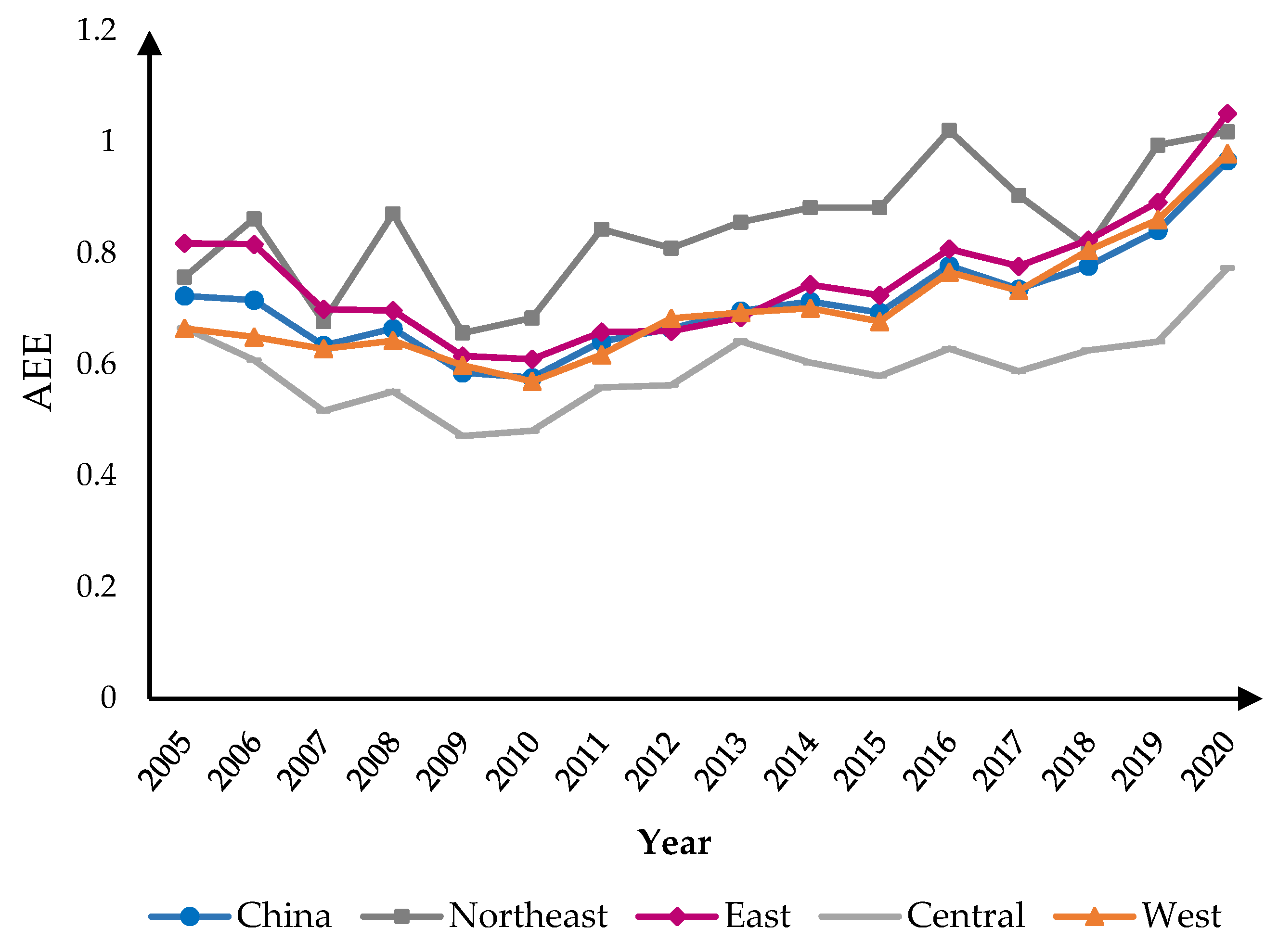
From 2005 to 2020, the provincial AEE in China ranged from 0.2839 to 1.1741 and had large time and regional dimensional differences. The eco-efficiency distribution in each region is shown in Figure 2.

China’s AEE first decreased and then increased, with the inflection point occurring in 2010, that is, the AEE development was U-shaped.

During the 11th Five-Year Plan period (2006–2010), as the dominant agricultural development philosophy in this period was aimed toward improving agricultural productivity and value-added capacity, the agricultural output-per-unit area and the intensification degree were low. During the 12th (2010–2015) and the 13th Five-Year Plans (2016–2020), the AEE was in an upward phase and grew faster in the latter five years. The AEE rise from 2011 to 2015 was mainly due to comprehensive rural environmental improvements, agricultural nonpoint source pollution prevention projects, and scientific guidance on the use of fertilizers and pesticides, all of which effectively promoted agricultural development, environmental protection, and energy conservation. During the 13th Five-Year Plan period, zero-growth fertilizer and pesticide-use actions and recycling agriculture combined with planting and raising projects were also implemented.

Of the four major regions, the eco-efficiencies in the northeast fluctuated slightly but were at the highest overall level, followed by the eastern region. The western region had more synchronized and slightly lower growth dynamics than the eastern region, and the AEE in the central region was the lowest, which was similar to the findings in [8,15].

The northeast region had an inherent resource advantage because of its fertile black soil. China’s grain production in 2021 was 685.58 billion tons, 21.2% of which was produced in the northeast [65], implying that this region had a high carbon sink for crops returned to the land. The large-scale agricultural intensification in the northeast also improved output efficiency. However, as agricultural production is relatively sensitive to climate, policy, and economic conditions, the northeast AEE fluctuated widely [5].

The eastern region is the most economically developed in China, with a high degree of industrialization and a more serious occupation of agricultural land resources. However, according to

Table A3. Average redundancy and insufficient ratio of agricultural inputs and outputs of four major regions in China.

Redundancy or Insufficient Ratio	Northeast	East	Central	West
Labor force (%)	1.6212	26.8652	32.8355	44.6325
Total crops-sown area (%)	12.5132	16.4746	29.5701	33.9869
Agricultural fiscal expenditure (%)	5.8691	14.3961	21.2435	19.5958
Total power of agricultural machinery (%)	7.7405	25.6820	30.7739	20.8063
Rural electricity consumption (%)	54.0179	56.1256	25.2780	25.3587
Effective irrigation area (%)	12.2323	29.3778	34.4833	21.4976
Gross agricultural output value (%)	3.5448	0.0869	1.3056	0.0138
Agricultural carbon sink value (%)	0.0000	3.2372	5.2825	0.9213
Agricultural carbon emissions (%)	6.4314	25.8045	41.9793	13.1367
Agricultural nonpoint source pollution (%)	7.5210	21.5806	25.5163	21.4308

Note: the input redundancy ratio equals “excessive input/total input”; the undesirable output redundancy rate equals “excessive undesirable output/total undesirable output”; the insufficient output ratio for desired output equals “insufficient output/total output”.

, the east had higher agricultural machinery power, irrigation area, and power usage redundancy ratio and a higher undesirable output redundancy ratio of carbon emissions and nonpoint source pollution. Therefore, its resource utilization was inefficient, which resulted in excessive carbon emissions and agricultural pollution. Therefore, the economic resource advantages of the eastern region were not fully reflected in its green agricultural development.

The western region’s efficiency had similar redundancies to the eastern region. However, it had the highest labor and crops-sown area redundancy ratio of the four regions (see Table A3), primarily related to its economic, geographic, and population backgrounds. Although the western region covers a large area, the agricultural farming conditions in the west are poorer than in other regions. Mechanization is low and labor is an important production factor, all of which contributed to the higher workforce and land redundancies.

Aside from rural electricity consumption, labor input, land input, and total agricultural output, the central region’s input and undesirable output redundancy rates were the highest of the four regions (see Table A3), indicating that the central region had significant agricultural materials, water, and land inefficiencies [8]. Additionally, its carbon sink insufficient rate was also the highest, indicating that a high carbonization of agricultural development was evident.

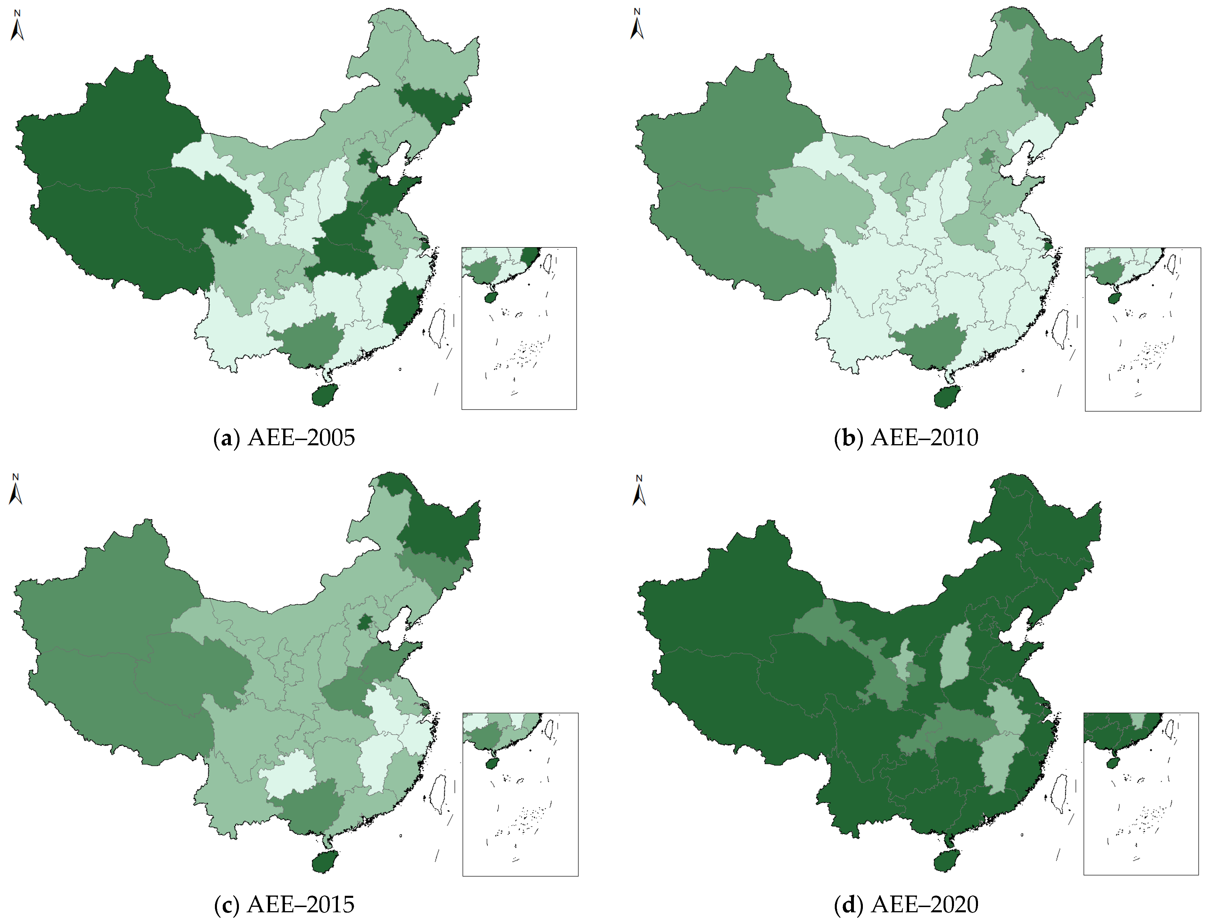
For a more intuitive reflection of the comparative AEEs in different regions and their respective development trends, a hierarchical map (Figure 3) was drawn using ArcGIS.

When the mean efficiencies in each province were ranked, the five highest AEE provinces were Beijing (E), Shanghai (E), Hainan (E), Xinjiang (W), and Inner Mongolia (W), and the five lowest were Jiangxi (C), Zhejiang (E), Anhui (C), Chongqing (W), and Guizhou (W). The best- and worst-performing regions did not show agglomeration, which indicated that there were large intra-regional variations.

Zhejiang Province had the highest average annual growth rate (8.51%). Before 2017, Zhejiang province had inefficient energy utility, excessive carbon emissions, and a low carbon sink value. However, after the optimization of these aspects, an effective state was attained in 2020. In contrast, the lowest average growth rate was in Hubei province (−1.62%), primarily because of the lack of improvements in its agricultural input and output structures.

4.2. Dynamic AEE Evaluation

4.2.1. Dynamic AEE Growth Rate

The dynamic AEE changes in the 31 provinces were evaluated and analyzed using the GML index. Due to the growth calculations involved, only 15 periods were evaluated over the 16 years, the results for which are shown in

Table 4. The results of GML, EC, and PBC indices for China in the years 2006–2020.

Period	GML	EC	PBC
2005–2006	0.9849	0.9358	1.0525
2006–2007	0.8896	1.0161	0.8755
2007–2008	1.0489	1.0528	0.9963
2008–2009	0.8885	0.9588	0.9266
2009–2010	0.9907	1.0192	0.9721
2010–2011	1.1071	0.9918	1.1162
2011–2012	1.0444	1.0196	1.0243
2012–2013	1.0502	1.0107	1.0391
2013–2014	1.0345	1.0100	1.0242
2014–2015	0.9841	1.0128	0.9717
2015–2016	1.1249	1.0083	1.1157
2016–2017	0.9491	0.9698	0.9787
2017–2018	1.0548	0.9999	1.0549
2018–2019	1.0897	1.0046	1.0846
2019–2020	1.1539	1.0111	1.1412
2006–2010 (11th Five-Year Plan)	0.9585	0.9956	0.9627
2011–2015 (12th Five-Year Plan)	1.0433	1.0090	1.0341
2016–2020 (13th Five-Year Plan)	1.0720	0.9986	1.0735
2006–2020 (all periods)	1.0235	1.0010	1.0224

and

Table 5. The results of GML, EC, and PBC indices for 31 provinces in China during 2006–2020.

Province	GML	EC	PBC	Rank
Liaoning (N)	1.0408	0.9984	1.0425	9
Jilin (N)	0.9987	0.9965	1.0021	28
Heilongjiang (N)	1.0275	1.0131	1.0142	12
Beijing (E)	1.0026	1.0408	0.9633	20
Tianjin (E)	1.0001	1.0119	0.9884	27
Hebei (E)	1.0261	1.0238	1.0023	14
Shanghai (E)	1.0021	0.9859	1.0165	24
Jiangsu (E)	1.0421	0.9976	1.0446	8
Zhejiang (E)	1.0851	1.0005	1.0846	1
Fujian (E)	1.0025	1.0012	1.0013	22
Shandong (E)	1.0024	0.9996	1.0028	23
Guangdong (E)	1.0655	0.9987	1.0669	2
Hainan (E)	1.0005	0.9931	1.0075	25
Shanxi (C)	1.0231	0.9746	1.0497	16
Anhui (C)	0.9941	0.9862	1.008	29
Jiangxi (C)	1.0185	0.9964	1.0222	17
Henan (C)	1.0026	0.9949	1.0077	21
Hubei (C)	0.9838	0.9816	1.0023	31
Hunan (C)	1.0532	0.9992	1.054	6
Inner Mongolia (W)	1.0312	1.0018	1.0294	11
Guangxi (W)	1.0153	1.0026	1.0127	18
Chongqing (W)	1.0271	0.9961	1.0311	13
Sichuan (W)	1.0491	1.0007	1.0484	7
Guizhou (W)	1.0615	1.0064	1.0548	4
Yunnan (W)	1.0552	1.0268	1.0277	5
Tibet (W)	0.9937	0.9594	1.0357	30
Shaanxi (W)	1.0633	1.0029	1.0603	3
Gansu (W)	1.0339	0.9815	1.0534	10
Qinghai (W)	1.0099	1.0244	0.9858	19
Ningxia (W)	1.0251	1.0426	0.9832	15
Xinjiang (W)	1.0005	0.998	1.0024	26
Northeast region	1.0222	1.0027	1.0195
Eastern region	1.0225	1.0052	1.0172
Central region	1.0123	0.9888	1.0238
Western region	1.0302	1.0034	1.0268
China	1.0235	1.0010	1.0224

.

GML index phase characteristics and component changes.

From 2005 to 2020, the average annual growth in the GML, PBC, and EC indices was 2.35%, 2.24%, and 0.1%, respectively. After a decline of 4.15% during the 11th Five-Year Plan period, annual GML index growth in the 12th and the 13th Five-Year Plan periods was 4.33% and 7.20%, respectively.

The main driving force for the AEE changes was technological progress. The Chinese government has always attached importance to developing agricultural science and technology [66]. Before 2010, government-led agricultural information technology guided production through information dissemination. After 2010, “internet plus agriculture” became dominant, and technologies such as agricultural e-commerce, the agricultural Internet of Things, and agricultural traceability were oriented toward market transactions and broadened agricultural product sales. More recently, artificial intelligence has been gradually applied to agriculture, such as seed detection, intelligent planting, crop monitoring, and soil irrigation, to improve agricultural production efficiencies and reduce costs. Statistically, mechanized farming has advanced significantly to 69.1%, and the rural internet penetration rate had improved from 0 to 38.4% by 2018. During the 13th Five-Year Plan period, the agricultural science and technology contribution rate exceeded 60% [67]. However, China’s agricultural digital technology has only been applied in a few fields, so there is significant room for improvement.

Interregional GML index characteristics and its component changes.

The average annual eco-efficiency growth rates in the northeast, eastern, central, and western regions were 2.22%, 2.25%, 1.23%, and 3.02%, respectively, of which the PBC contributed 1.95%, 1.72%, 2.38%, and 2.68%, respectively, and the EC contributed less than 0.6%. The EC in the central region reduced by 1.2%, indicating that the input factor coordination was not high, and its technical potential was not yet realized.

The Chinese provinces were classified into three categories based on reasons for the eco-efficiency changes. The first category included provinces in which technical efficiency played a major role: Beijing, Tianjin, Hebei, Qinghai, and Ningxia. These four provinces had an average EC greater than 1 but a PBC of less than 1. The second category comprised provinces in which both technical efficiency and technological progress played joint roles, Heilongjiang, Fujian, and Yunnan, and both EC and PBC positively contributed and had similar effects on the eco-efficiency dynamics. The third category involved provinces where technological progress played a dominant role, with all the remaining 23 provinces falling into this category. While the AEE drivers were found to vary in the Chinese provinces, technological progress was the predominant driver, indicating that the technical efficiency drivers played relatively minor roles and existing resource allocation and coordination approaches need to be urgently optimized to enhance resource utilization efficiencies.

4.2.2. Kernel Density Estimation of AEE

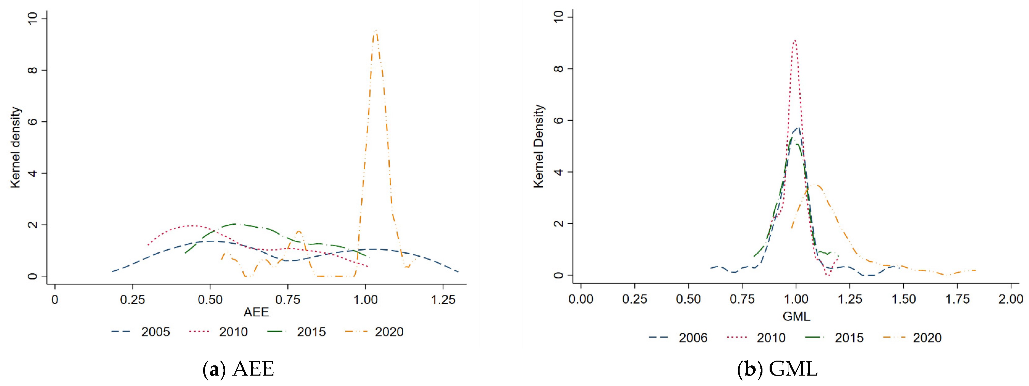
Figure 4a shows the results for the kernel density AEE estimations. From the density function center (the value corresponding to the horizontal coordinate), the kernel value in 2020 was the largest, indicating that the average AEE in 2020 was the highest in four years. Aside from that of 2010, the kernel density distribution curves all showed a flattening trend to the right, revealing an AEE trend from decline to rise. The peak density center value in 2020 was more prominent and had a longer tail on the left side, showing that more provinces were nearer to the average value and there were greater efficiency variations in the provinces below the mean. There was only one evident peak in 2020, but in 2005, 2010, and 2015, there were double peaks and the curves were flatter. Therefore, the AEE distribution was characterized by an overall dispersion and concentration in individual years.

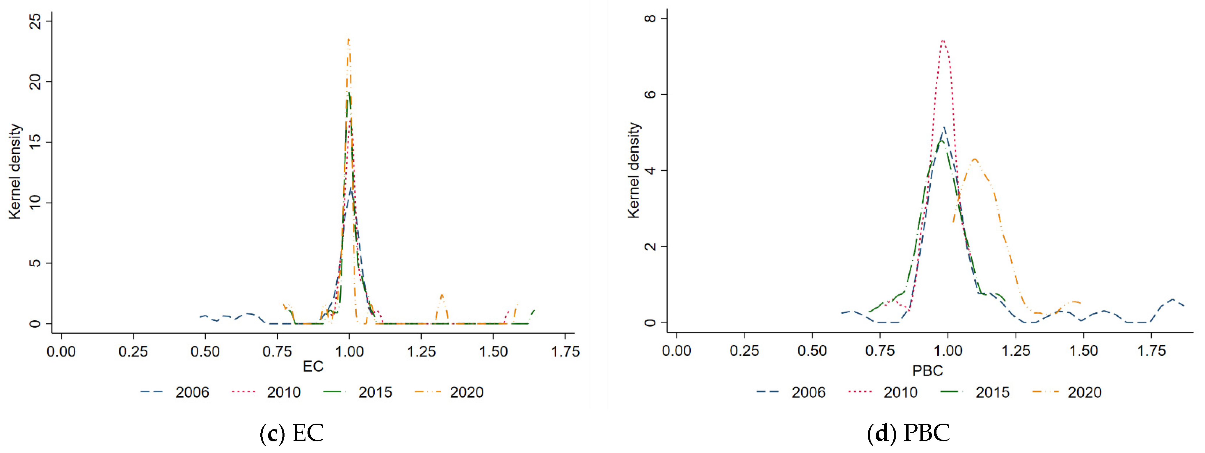
Figure 4b–d show the GML, EC, and PBC distributions. The GML and the PBC index kernel density curves were similar, the overall distribution was more concentrated in 2005, 2010, and 2015, and the density function center shifted significantly to the right in 2020, indicating that both the GML and PBC indices increased significantly in 2020. The GML and PBC indices showed significant single-wave crest conditions at 1 in 2006, 2010, and 2015, that is, their mean values were concentrated around 1. However, in 2020, there was a clear single-wave peak with a long right tail, which suggested that more provinces were concentrated near the mean and the eco-efficiency differences in the provinces above the mean were widening.

The technical efficiency (EC) kernel density distribution curve was concentrated around 1 and had little variation over the years. All four years had significant single-wave peak conditions, with the wave height increasing each year, which illustrated that the technical efficiency distribution concentration was increasing and there were few inter-regional variations.

In summary, there were more obvious eco-efficiency growth trends, with the eco-efficiency moving from being decentralized to being centralized. The growth rate for the AEE (GML) and technical progress (PBC) moved from being centralized to being dispersed and the regional differences were enhanced, with the technical progress being more evident in some provinces. The technical efficiency (EC) distribution was more concentrated, and the change magnitude was small. Therefore, the kernel density estimation once again verified that the main contribution to the AEE changes was related to the increase in technical progress.

4.3. Spatial Distribution Characteristics of AEE

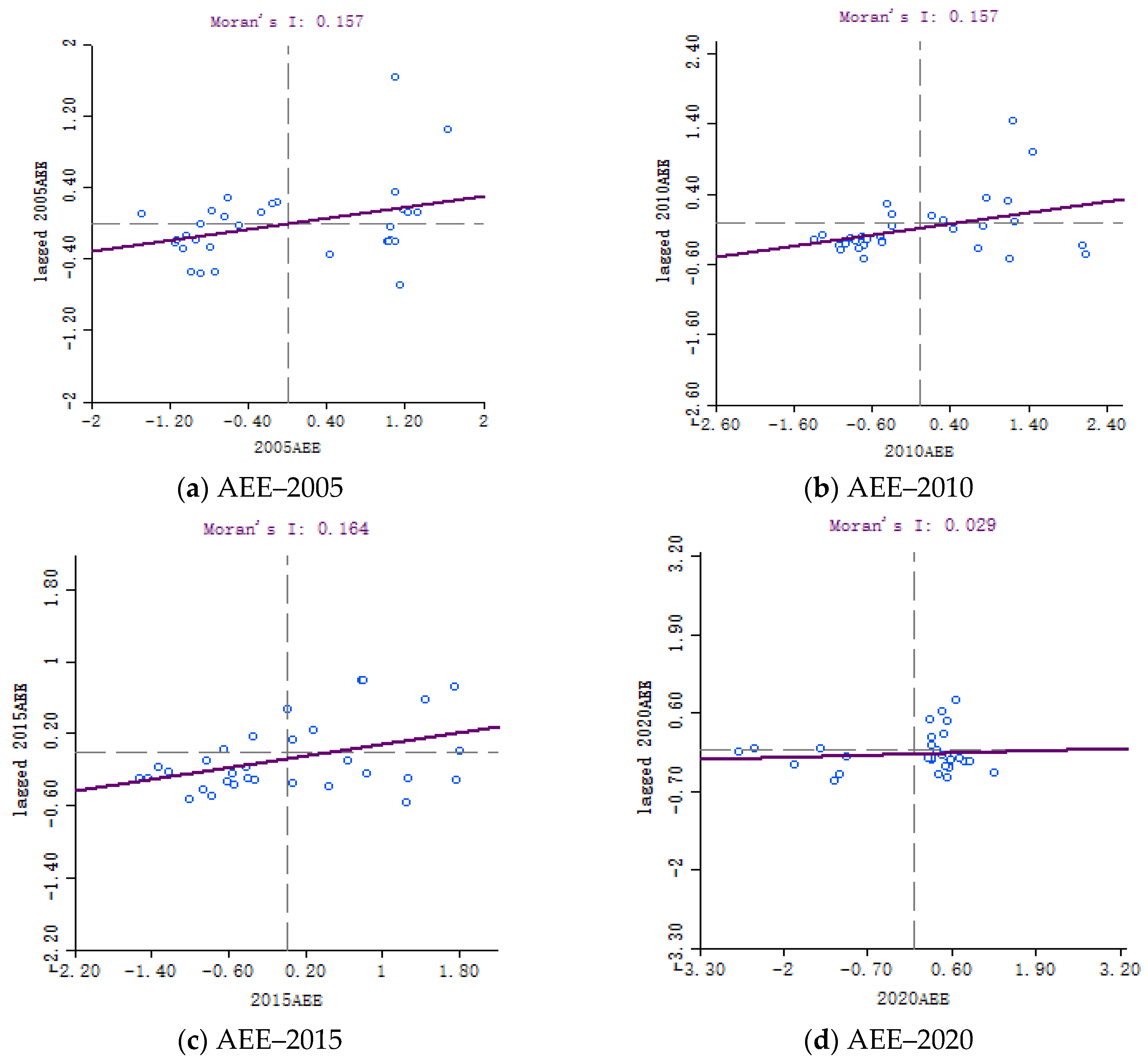
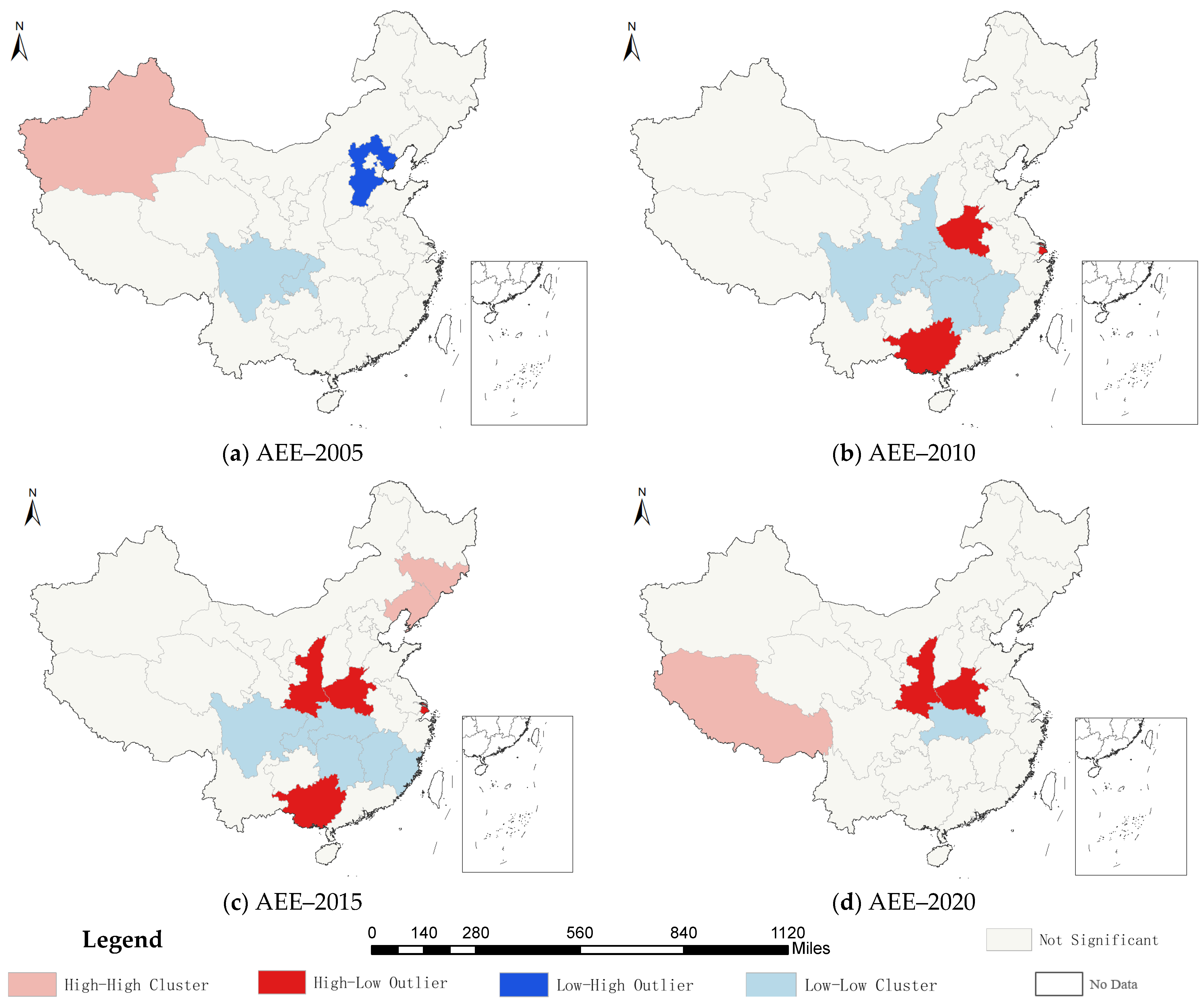
The exploratory spatial data analysis (ESDA) focused on the spatial autocorrelation of the AEE. The global Moran index (

Table 6. The results of Moran’s I of agricultural eco-efficiency in China from 2005 to 2020.

Year	Moran’s I	z	p	Year	Moran’s I	z	p
2005	0.1574	2.2450	0.0180	2013	0.0943	1.5816	0.0590
2006	0.1566	2.2590	0.0200	2014	0.1045	1.8089	0.0460
2007	0.1519	2.1258	0.0190	2015	0.1640	2.4439	0.0140
2008	0.1963	2.7319	0.0070	2016	0.2994	3.8808	0.0020
2009	0.1828	2.8050	0.0070	2017	0.0936	1.5866	0.0540
2010	0.1572	2.3736	0.0160	2018	0.0839	1.4615	0.0720
2011	0.1887	2.7365	0.0090	2019	0.1432	2.1319	0.0190
2012	0.1610	2.4314	0.0120	2020	0.0291	0.6919	0.1900

), the local Moran scatterplot (Figure 5), and the local indicators of spatial association (LISA Figure 6) for AEE from 2005 to 2020 were determined using ArcGIS.

Table 6 shows that the global Moran index for China’s AEE from 2005 to 2019 ranged from 0.0839 to 0.2994, all of which were significant at least at the 10% level. Although the degree of spatial correlation varied, there were always significant spatial effects, which indicated that the Chinese provincial AEEs had significant positive spatial correlations. The eco-efficiency was possibly influenced by spatial spillovers from neighboring provinces, that is, there was a demonstration effect. However, the Moran’s I for 2020 was insignificant, meaning there were no significant spatial autocorrelations.

To clarify the association characteristics of each province to its neighboring provinces, a Moran scatter plot and a LISA agglomeration plot were constructed to reveal the local association patterns. Figure 5 shows that China’s AEE was mainly concentrated in the first quadrant (H-H clustering), the third quadrant (L-L clustering), and the fourth quadrant (H-L clustering).

According to Figure 6, in 2005, the main distribution features were H-H clustering (Xinjiang) and L-L clustering (Sichuan and Chongqing), both in the western region. These patterns illustrated that the agricultural technology and the input-output structures in neighboring provinces gradually converged, meaning there were fewer spatial differences [4]. Hebei had L-H clustering, probably because the unidirectional flow of Hebei’s resources to Beijing and Tianjin led to a lack of technical and agricultural talent development support, which regressed the ecological efficiency.

In 2010, the L-L and H-L agglomerations were significant. Compared with 2005, the L-L zone expanded and formed a contiguous trend to span three regions from the east to the west, including Shaanxi, Chongqing, Hunan, Hubei, Jiangxi, and Fujian. This outcome indicated that, because rapid urbanization had reduced the availability of high-quality arable land, agricultural development became more focused on yield but neglected sustainable development. The H-L agglomeration was mainly distributed in Guangxi, Henan, and Shanghai, indicating that the high center region AEE had exerted a siphoning effect on the surrounding disadvantaged areas, which widened the gaps with the neighboring provinces.

In 2015, Shaanxi Province shifted from an L-L to an H-L agglomeration, Jilin and Liaoning showed significant H-H agglomeration, Sichuan Province returned to a significant L-L clustering, and Hebei Province moved away from an L-L agglomeration. The possible reasons for these changes were that Shaanxi Province, with the help of western development and the Belt and Road Strategy, had policy advantages and had prioritized green transformation; however, Sichuan and its neighboring provinces had less collaborative capacity and had not realized any complementary agricultural production advantages. In contrast, the Beijing-Tianjin-Hebei region’s strategy that was focused on collaborative pollution control had enhanced overall low-carbon agricultural development.

In 2020, the AEE distribution was mainly dominated by H-H, H-L, and L-L clustering. As Tibet (H-H clustering) is an important ecological security barrier in China, the government has attached importance to its ecological construction. Consequently, to keep Tibet one of the best ecological regions in the world, a good green agricultural development foundation has been built. H-L clustering was found mainly in Shaanxi and Henan, but Hubei province still had an L-L agglomeration.

4.4. Convergence Analysis of AEE

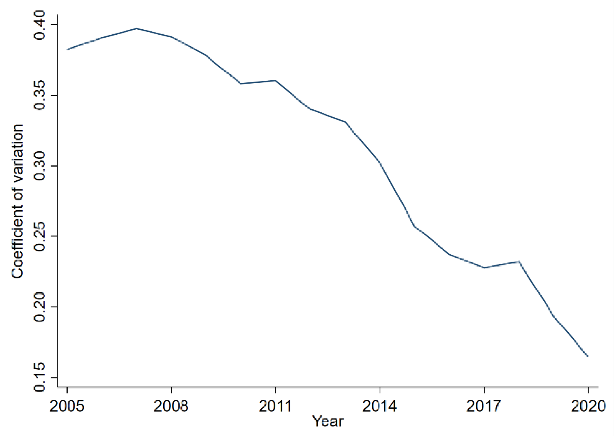
$\mathsf{\delta }$ convergence was measured using the coefficient of variation, the results of which are shown in Figure 7. The AEE coefficient of variation fluctuated and decreased from 2005 to 2020, which indicated that the AEE differences between the provinces were narrowing.

Table 7. The results of absolute and conditional $\mathsf{\beta }$ convergence for agricultural eco-efficiency in China.

Variable	$$\mathbf{Absolute}\mathsf{\beta }\mathbf{Convergence}$$	$$\mathbf{Conditional}\mathsf{\beta }\mathbf{Convergence}$$
L.AEE	−0.2078 **	−0.3490 ***
	(−2.4300)	(−4.7000)
lndpi		0.0835 ***
		(6.7600)
lnmech		−0.1164 ***
		(−2.8400)
haz		−0.0015 **
		(−2.2400)
lndigit		0.0127
		(0.5400)
cons	0.1608 **	−0.5028 *
	(2.7000)	(−1.7600)
N	465	465
Adjusted R2	0.0560	0.2583
F-test	5.8915	23.3408
Model	FE	FE
Hausman Test	11.71	62.33
(p-value)	0.0006	0.0000

Note: * p < 0.1, ** p < 0.05, *** p < 0.01; L.AEE is the lagged term of AEE; standard errors are in parentheses.

shows that the initial AEE for the β absolute convergence model was significant at a 5% confidence level, and the AEE coefficient was less than 0.

The control variables, rural household per capita disposable income (dpi), total mechanical power per unit area (mech), the percentage of area affected by natural disasters (haz), and digital concern (digit), were applied in the conditional β convergence model, with the dpi being adjusted using the agricultural product price index, and the dpi, mech, and digit being logarized. Similarly, the initial AEE for the conditional β convergence model was significantly negative at the 1% level, and the convergence rate was accelerated (0.3490 > 0.2078), which demonstrated that the AEE in the Chinese provinces was converging to the same level and there was a catch-up effect.

There was a significant positive relationship between rural households’ per capita disposable income and the AEE changes. Higher disposable income ensures that agricultural producers have access to more agricultural production resources, such as capital and farming tools, which enhances their agricultural productivity. Higher income also facilitates agricultural producers to pay greater attention to the production and consumption of green products, which directly or indirectly promotes AEE improvements. The impacts of agricultural mechanization and the affected area percentage on the AEE were negative and significant at 1% and 5%. There were several reasons for these results. First, agricultural machinery inputs amplified diesel and gasoline consumption, which increased both carbon emissions and agricultural pollutants [13]; an over-reliance on mechanical power to exploit land potential without incorporating arable land systems, such as fallow or shifting cultivation, can be detrimental to AEE improvements. Second, any expansion of the affected agricultural areas could lead to insufficient output, wasted inputs, and a reduction in AEE [64]. The effect of local governments’ digital technology attention on AEE was positive but not significant, which suggested that technological attention has not yet become an important driver of green agricultural production and consumption.

5. Conclusions

5.1. Study Conclusion

This study investigated the static, dynamic, spatial, and convergent characteristics of AEE in China from 2005 to 2020. Based on the results, the following conclusions were drawn. First, Chinese AEE showed an overall U-shaped trend, with the inflection point occurring in 2010. The AEE had a downward trend during the 11th Five-Year Plan and an upward trend during the 12th and 13th Five-Year Plans. The non-equilibrium distribution revealed a “northeast > east > west > central” regional pattern. Second, the main driving factor for the AEE changes was found to be technological progress. Technical efficiency improvements were only found in some provinces and there was a significant technical efficiency decline in the central region. Third, the AEE was found to have an evident spatial autocorrelation, with H-H, L-L, and H-L clustering being the main characteristics. Finally, the per capita disposable income of rural residents weakened the AEE convergence, the agricultural mechanization and crop disaster area intensities reduced the eco-efficiencies and further narrowed the eco-efficiency differences between provinces, and there was an obvious “catch-up effect” in the lagging provinces.

5.2. Policy Recommendations

Some policy implications can be derived from our empirical study for the formulation of agricultural carbon reduction policies: First, it is important to continue promoting the integration of regional strategies and low-carbon development, such as the rise of central China, the western development drive, and the revitalization of northeast China, to reduce green development differences. Because the eastern region has solid economic and scientific support, encouraging the east to cooperate with other regions on joint research and development on agricultural emission reduction and carbon sequestration is critical. Further, a unified national agriculture market is needed to avoid the expansion of the Matthew effect and the digital agriculture divide, that is, it is essential to develop agricultural production by promoting coordinated regional and urban-rural development and to enhance agricultural producers’ incomes through the free flow of factors.

Second, the establishment of a low-carbon technology support system for agriculture is crucial. As agricultural production relies heavily on energy-consuming industrial products, more attention needs to be paid to the exploration and application of clean energy and eco-friendly materials. Agricultural production needs to change from input and output quantity orientations to high-quality development and improve resource utilization efficiency. Certain measures could be adopted to encourage agricultural producers to implement low-carbon agricultural technologies, such as balanced fertilization, organic fertilizer application, and straw return. Further, to enhance agricultural disaster resistance and mitigation capabilities and ensure the sustainable and healthy development of the agricultural industry, a complete agricultural disaster monitoring and early-warning information system is needed to ensure the stockpiling of production materials.

Third, low-carbon agricultural production and consumption are essential for the achievement of double carbon goals. Xiamen’s experience should be drawn on to accelerate the construction of a national agricultural carbon trading center. In conjunction with this, an inventory of agricultural carbon sources and sinks should be compiled, and the monitoring, accounting, and reporting system for agricultural carbon emissions data needs to be improved. Opening of the carbon trading market to facilitate the realization of agricultural ecological values and guide low-carbon production should be promoted. The government should urgently develop a carbon labeling system for agricultural products and formulate corresponding subsidy policies. The establishment of green brands of agriculture products, the attracting of consumer purchasing power, and the expansion of market influence with identifiable labels are needed.

5.3. Limitations and Future Research

Although this paper is innovative in its indicator construction, it still had some limitations. First, there are large geographical, meteorological, and economic disparities between the 31 provinces. Due to the long span of the study, the conversion coefficients of different periods will be different. The adoption of uniform carbon emission coefficients and carbon absorption rates may lead to biased results. Second, China’s agricultural development is closely related to rural areas and farmers, and with the all-round implementation of the rural revitalization strategy, resources are gathering in rural areas and providing support for agricultural development. Therefore, more important indicators should be included in the research system, such as institutional or social factors that affect the agricultural structure and environment.

Some of the further research opportunities are as follows. First, the calculation of carbon emission coefficients and carbon absorption coefficients combined with the temporal and spatial characteristics of Chinese agriculture is a difficult and fundamental task, which is conducive to the accurate measurement of carbon sinks and carbon emissions. In this way, the assessment of low-carbon development efficiency will be more in-depth and can provide clearer guidelines for policy formulation. Second, as China has divided different functional grain production zones and important agricultural production reserves, allowing the same type of grain regions as decision-making units can improve the comparability of assessment results. Meanwhile, the index selection can be further optimized. External indicators such as rural areas and farmers are considered to provide a more comprehensive analysis of efficiency differences and low-carbon agricultural development. Finally, although agricultural carbon trading practices have been carried out successively in various pilot provinces, systematic research on agricultural carbon trading is lacking. Future research can combine domestic and international experience to explore how to build China’s national agricultural carbon trading center. Further, carrying out related policy evaluation is essential to promoting agricultural low-carbon transition.

References

1. Cui, Y.; Khan, S.U.; Deng, Y.; Zhao, M. Spatiotemporal heterogeneity, convergence and its impact factors: Perspective of carbon emission intensity and carbon emission per capita considering carbon sink effect. Environ. Impact Assess. Rev. 2022, 92, 106699. [Google Scholar] [CrossRef]
2. FAO News Article: Food Systems Account for More than One Third of Global Greenhouse Gas Emissions. Available online: https://www.fao.org/news/story/en/item/1379373/icode/ (accessed on 29 September 2022).
3. IPCC Special Report on Climate Change and Land. Available online: https://www.ipcc.ch/srccl/ (accessed on 27 September 2022).
4. Jin, G.; Li, Z.; Deng, X.; Yang, J.; Chen, D.; Li, W. An analysis of spatiotemporal patterns in Chinese agricultural productivity between 2004 and 2014. Ecol. Indic. 2019, 105, 591–600. [Google Scholar] [CrossRef]
5. Liu, Y.; Zou, L.; Wang, Y. Spatial-temporal characteristics and influencing factors of agricultural eco-efficiency in China in recent 40 years. Land Use Policy 2020, 97, 104794. [Google Scholar] [CrossRef]
6. Zou, L.; Liu, Y.; Wang, Y.; Hu, X. Assessment and analysis of agricultural non-point source pollution loads in China: 1978–2017. J. Environ. Manag. 2020, 263, 110400. [Google Scholar] [CrossRef]
7. Ministry of Agriculture and Rural Affairs. 2019 National Arable Land Quality Rating Bulletin. Available online: https://www.moa.gov.cn/nybgb/2020/202004/202005/t20200506_6343095.htm (accessed on 2 November 2022).
8. Wang, Y.; Shen, N. Agricultural environmental efficiency and agricultural Environmental Kuznets Curve based on technological gap: The case of China. Pol. J. Environ. Stud. 2016, 25, 1293–1303. [Google Scholar] [CrossRef] [PubMed]
9. Ministry of Agriculture and Rural Affairs. The Utilization Rate of Chemical Fertilizers and Pesticides for China’s Three Major Food Crops Both Exceeded 40 Percent. Available online: http://www.kjs.moa.gov.cn/gzdt/202101/t20210119_6360102.htm (accessed on 2 November 2022).
10. West, T.O.; Marland, G. A synthesis of carbon sequestration, carbon emissions, and net carbon flux in agriculture: Comparing tillage practices in the United States. Agric. Ecosyst. Environ. 2002, 91, 217–232. [Google Scholar] [CrossRef]
11. Chen, R.; Zhang, R.; Han, H.; Jiang, Z. Is farmers’ agricultural production a carbon sink or source?—Variable system boundary and household survey data. J. Clean. Prod. 2020, 266, 122108. [Google Scholar] [CrossRef]
12. Ministry of Agriculture and Rural Affairs. The Issuance of the 14th Five-Year Plan for National Green Development of Agriculture. Available online: https://www.moa.gov.cn/govpublic/FZJHS/202109/t20210907_6375844.htm (accessed on 2 November 2022).
13. Pishgar-Komleh, S.H.; Čechura, L.; Kuzmenko, E. Investigating the dynamic eco-efficiency in agriculture sector of the European Union countries. Environ. Sci. Pollut. Res. 2021, 28, 48942–48954. [Google Scholar] [CrossRef]
14. Ji, H.; Hoti, A. Green economy based perspective of low-carbon agriculture growth for total factor energy efficiency improvement. Int. J. Syst. Assur. Eng. Manag. 2022, 13, 353–363. [Google Scholar] [CrossRef]
15. Wu, G.; Fan, Y.; Riaz, N. Spatial analysis of agriculture ecological efficiency and its influence on fiscal expenditures. Sustainability 2022, 14, 9994. [Google Scholar] [CrossRef]
16. Zhuang, X.; Li, Z.; Zheng, R.; Na, S.; Zhou, Y. Research on the efficiency and improvement of rural development in China: Based on two-stage network SBM model. Sustainability 2021, 13, 2914. [Google Scholar] [CrossRef]
17. Cecchini, L.; Venanzi, S.; Pierri, A.; Chiorri, M. Environmental efficiency analysis and estimation of CO2 abatement costs in dairy cattle farms in Umbria (Italy): A SBM-DEA model with undesirable output. J. Clean. Prod. 2018, 197, 895–907. [Google Scholar] [CrossRef]
18. Rosano Peña, C.; Serrano, A.L.M.; de Britto, P.A.P.; Franco, V.R.; Guarnieri, P.; Thomé, K.M. Environmental preservation costs and eco-efficiency in Amazonian agriculture: Application of Hyperbolic Distance Functions. J. Clean. Prod. 2018, 197, 699–707. [Google Scholar] [CrossRef]
19. Wang, G.; Mi, L.; Hu, J.; Qian, Z. Spatial analysis of agricultural eco-efficiency and high-quality development in China. Front. Environ. Sci. 2022, 10, 193. [Google Scholar] [CrossRef]
20. Chi, M.; Guo, Q.; Mi, L.; Wang, G.; Song, W. Spatial distribution of agricultural eco-efficiency and agriculture high-quality development in China. Land 2022, 11, 722. [Google Scholar] [CrossRef]
21. Wu, G.; Xie, Y.; Li, H.; Riaz, N. Agricultural ecological efficiency under the carbon emissions trading system in China: A spatial Difference-in-Difference approach. Sustainability 2022, 14, 4707. [Google Scholar] [CrossRef]
22. Liu, Z.; Xin, L. Has China’s Belt and Road Initiative promoted its green total factor productivity? –Evidence from primary provinces along the route. Energy Policy 2019, 129, 360–369. [Google Scholar] [CrossRef]
23. Ma, X.; Wang, C.; Yu, Y.; Li, Y.; Dong, B.; Zhang, X.; Niu, X.; Yang, Q.; Chen, R.; Li, Y.; et al. Ecological efficiency in China and its influencing factors—A super-efficient SBM Metafrontier-Malmquist-Tobit model study. Environ. Sci. Pollut. Res. 2018, 25, 20880–20898. [Google Scholar] [CrossRef]
24. Liu, Y.; Sun, H.; Shi, L.; Wang, H.; Xiu, Z.; Qiu, X.; Chang, H.; Xie, Y.; Wang, Y.; Wang, C. Spatial-temporal changes and driving factors of land-use eco-efficiency incorporating ecosystem services in China. Sustainability 2021, 13, 728. [Google Scholar] [CrossRef]
25. Fang, L.; Hu, R.; Mao, H.; Chen, S. How crop insurance influences agricultural green total factor productivity: Evidence from Chinese farmers. J. Clean. Prod. 2021, 321, 128977. [Google Scholar] [CrossRef]
26. Cao, L.; Zhou, Z.; Wu, Y.; Huang, Y.; Cao, G. Is metabolism in all regions of China performing well?—Evidence from a new DEA-Malmquist productivity approach. Ecol. Indic. 2019, 106, 105487. [Google Scholar] [CrossRef]
27. Shi, H.; Li, P.; Wei, J.; Shi, S. Green growth efficiency evaluation of major domestic oil-gas resource-based cities—Based on panel data of SBM model and Malmquist-Luenberger index. Front. Earth Sci. 2022, 10, 863. [Google Scholar] [CrossRef]
28. Schaltegger, S.; Sturm, A. Ökologische Rationalität: Ansatzpunkte Zur Ausgestaltung von Ökologieorientierten Managementinstrumenten. Die. Unternehm. 1990, 44, 273–290. Available online: https://www.jstor.org/stable/24180467 (accessed on 1 October 2022).
29. UNESCAP. Eco-Efficiency Indicators: Measuring Resource-Use Efficiency and the Impact of Economic Activities on the Environment. Available online: https://sustainabledevelopment.un.org/index.php?page=view&type=400&nr=785&menu=1515 (accessed on 8 October 2022).
30. Wang, G.; Shi, R.; Mi, L.; Hu, J. Agricultural eco-efficiency: Challenges and progress. Sustainability 2022, 14, 1051. [Google Scholar] [CrossRef]
31. Pang, J.; Chen, X.; Zhang, Z.; Li, H. Measuring eco-efficiency of agriculture in China. Sustainability 2016, 8, 398. [Google Scholar] [CrossRef] [Green Version]
32. ISO 14040: 2006. Available online: https://www.iso.org/cms/render/live/en/sites/isoorg/contents/data/standard/03/74/37456.html (accessed on 2 October 2022).
33. Bouman, M.; Heijungs, R.; van der Voet, E.; van den Bergh, J.C.J.M.; Huppes, G. Material flows and economic models: An analytical comparison of SFA, LCA and Partial Equilibrium models. Ecol. Econ. 2000, 32, 195–216. [Google Scholar] [CrossRef]
34. Moutinho, V.; Robaina, M.; Macedo, P. Economic-environmental efficiency of European agriculture—A generalized maximum entropy approach. Agric. Econ. 2018, 64, 423–435. [Google Scholar] [CrossRef] [Green Version]
35. Liu, S.; Xiao, W.; Li, L.; Ye, Y.; Song, X. Urban land use efficiency and improvement potential in China: A Stochastic Frontier Analysis. Land Use Policy 2020, 99, 105046. [Google Scholar] [CrossRef]
36. Charnes, A.; Cooper, W.W.; Rhodes, E. Measuring the efficiency of decision making units. Eur. J. Oper. Res. 1978, 2, 429–444. [Google Scholar] [CrossRef]
37. Zhang, N.; Zhang, G.; Li, Y. Does major agriculture production zone have higher carbon efficiency and abatement cost under climate change mitigation? Ecol. Indic. 2019, 105, 376–385. [Google Scholar] [CrossRef]
38. Wang, Y.; Chen, X. Natural resource endowment and ecological efficiency in China: Revisiting resource curse in the context of ecological efficiency. Resour. Policy 2020, 66, 101610. [Google Scholar] [CrossRef]
39. Hou, J.; Ruan, X.; Lv, J.; Guo, H. Two-stage super-efficiency Slacks-Based model to assess China’s ecological wellbeing. Int. J. Environ. Res. Public Health 2020, 17, 7045. [Google Scholar] [CrossRef] [PubMed]
40. Lee, P.; Park, Y.-J. Eco-efficiency evaluation considering environmental stringency. Sustainability 2017, 9, 661. [Google Scholar] [CrossRef] [Green Version]
41. Ouenniche, J.; Carrales, S. Assessing efficiency profiles of UK commercial banks: A DEA analysis with regression-based feedback. Ann. Oper. Res. 2018, 266, 551–587. [Google Scholar] [CrossRef] [Green Version]
42. Banker, R.D.; Charnes, A.; Cooper, W.W. Some models for estimating technical and scale inefficiencies in Data Envelopment Analysis. Manage. Sci. 1984, 30, 1078–1092. [Google Scholar] [CrossRef] [Green Version]
43. Tone, K. A Slacks-Based Measure of super-efficiency in Data Envelopment Analysis. Eur. J. Oper. Res. 2002, 143, 32–41. [Google Scholar] [CrossRef] [Green Version]
44. Tone, K. Dealing with undesirable outputs in DEA: A Slacks-Based Measure (SBM) approach. Nippon Opereshonzu, Risachi Gakkai Shunki Kenkyu Happyokai Abusutorakutoshu. Present. NAPW III Tor. 2004, 1, 44–45. Available online: https://www.researchgate.net/publication/284047010_Dealing_with_undesirable_outputs_in_DEA_a_Slacks-Based_Measure_SBM_approach (accessed on 3 October 2022).
45. Hong, Q.; Cui, L.; Hong, P. The impact of carbon emissions trading on energy efficiency: Evidence from quasi-experiment in China’s carbon emissions trading pilot. Energy Econ. 2022, 110, 106025. [Google Scholar] [CrossRef]
46. Li, Y.; Chen, Y. Development of an SBM-ML model for the measurement of green total factor productivity: The case of Pearl River delta urban agglomeration. Renew. Sust. Energy Rev. 2021, 145, 111131. [Google Scholar] [CrossRef]
47. Hao, Z.; Ye, D.; Hui, W.; Han, Z.; Wang, H. An empirical analysis of tourism eco-efficiency in ecological protection priority areas based on the DPSIR-SBM model: A case study of the Yellow River basin, China. Ecol. Inform. 2022, 70, 101720. [Google Scholar] [CrossRef]
48. Huang, J.; Yang, X.; Cheng, G.; Wang, S. A comprehensive eco-efficiency model and dynamics of regional eco-efficiency in China. J. Clean. Prod. 2014, 67, 228–238. [Google Scholar] [CrossRef]
49. Cheng, K.; Li, S. Total factor productivity indices: Evolution, comparison and prospect. J. Stat. 2022, 3, 11–26. [Google Scholar] [CrossRef]
50. Kortelainen, M. Dynamic environmental performance analysis: A Malmquist index approach. Ecol. Econ. 2008, 64, 701–715. [Google Scholar] [CrossRef]
51. Pastor, J.T.; Lovell, C.A.K. A global Malmquist productivity index. Econ. Lett. 2005, 88, 266–271. [Google Scholar] [CrossRef]
52. Oh, D. A Global Malmquist-Luenberger productivity index. J. Prod. Anal. 2010, 34, 183–197. [Google Scholar] [CrossRef]
53. Yang, C.; Li, T.; Albitar, K. Does energy efficiency affect ambient PM2.5? The moderating role of energy investment. Front. Environ. Sci. 2021, 9, 210. [Google Scholar] [CrossRef]
54. Yao, Y.; Hu, D.; Yang, C.; Tan, Y.; Yao, Y.; Hu, D.; Yang, C.; Tan, Y. The impact and mechanism of fintech on green total factor productivity. Green Financ. 2021, 3, 198–221. [Google Scholar] [CrossRef]
55. Liu, J.; Wang, H.; Ho, H.; Huang, L. Impact of heterogeneous environmental regulation on manufacturing sector green transformation and sustainability. Front. Environ. Sci. 2022, 10, 933. [Google Scholar] [CrossRef]
56. Deng, X.; Gibson, J. Improving eco-efficiency for the sustainable agricultural production: A case study in Shandong, China. Technol. Forecast. Soc. Chang. 2019, 144, 394–400. [Google Scholar] [CrossRef]
57. National Bureau of Statistics of China. Consultation on the Classification of Chinese Provinces. Available online: http://www.stats.gov.cn/tjfw/tjzx/tjzxbd/201811/t20181110_1632622.html (accessed on 29 November 2022).
58. Golany, B.; Roll, Y. An application procedure for DEA. Omega 1989, 17, 237–250. [Google Scholar] [CrossRef]
59. Wang, B.; Zhang, W. Cross-provincial differences in determinants of agricultural eco-efficiency in China: An analysis based on panel data from 31 provinces in 1996–2015. Chin. Rural. Econ. 2018, 1, 46–62. Available online: http://crecrs-zgncjj.ajcass.org/Magazine/Show/52958 (accessed on 5 October 2022).
60. Li, B.; Zhang, J.; Li, H. Research on spatial-temporal characteristics and affecting factors decomposition of agricultural carbon emission in China. Chin. J. Popul. Resour. Environ. 2011, 21, 80–86. Available online: http://www.cpre.sdnu.edu.cn/WKC/WebPublication/paperDigest.aspx?paperID=36bebf03-46d1-4b80-aeb2-128f90e85179 (accessed on 10 October 2022).
61. Wu, X.; Zhang, J.; Tian, Y.; Li, P. Provincial agricultural carbon emissions in China: Calculation, performance change and influencing factors. Resour. Sci. 2014, 36, 129–138. Available online: https://kns.cnki.net/kcms/detail/detail.aspx?dbcode=CJFD&dbname=CJFD2014&filename=ZRZY201401015&uniplatform=NZKPT&v=Ruv3NxuWrnmx4-P0SAkEeiu-CDn87wt5Jv2c7EwluWgqDlp_4jttRFsBgrnQyTNY (accessed on 5 October 2022).
62. Färe, R.; Grosskopf, S.; Pasurka, C.A. Environmental production functions and environmental Directional Distance Functions. Energy 2007, 32, 1055–1066. [Google Scholar] [CrossRef]
63. Fukuyama, H.; Weber, W.L. A directional Slacks-Based Measure of technical inefficiency. Socio Econ. Plan. Sci. 2009, 43, 274–287. [Google Scholar] [CrossRef]
64. Guo, L.; Du, S.; Haining, R.; Zhang, L. Global and local indicators of spatial association between points and polygons: A study of land use change. Int. J. Appl. Earth Obs. Geoinf. 2013, 21, 384–396. [Google Scholar] [CrossRef]
65. National Bureau of Statistics of China Bulletin on the National Grain Output in 2021. Available online: http://www.stats.gov.cn/english/PressRelease/202112/t20211207_1825086.html (accessed on 2 November 2022).
66. Du, J.; Wang, R.; Wang, X. Environmental total factor productivity and agricultural growth: A two-stage analysis based on DEA-GML index and panel Tobit model. Chin. Rural. Econ. 2016, 03, 65–81. Available online: http://crecrs-zgncjj.ajcass.org/Magazine/Show/14394 (accessed on 1 November 2022).
67. Ministry of Agriculture and Rural Affairs. Great Changes in Agriculture and Rural Areas in New China at 70. Available online: https://www.moa.gov.cn/xw/zwdt/201911/t20191114_6331856.htm (accessed on 2 November 2022).
68. Tian, Y.; Zhang, J. Regional differentiation research on net carbon effect of agricultural production in China. J. Nat. Resour. 2013, 28, 1298–1309. Available online: http://www.jnr.ac.cn/CN/Y2013/V28/I8/1298 (accessed on 1 November 2022).
69. Dubey, A.; Lal, R. Carbon footprint and sustainability of agricultural production systems in Punjab, India, and Ohio, USA. J. Crop Improv. 2009, 23, 332–350. [Google Scholar] [CrossRef]
70. Wang, M.-X.; Shangguan, X.-J. CH4 Emission from various rice fields in P.R. China. Theor. Appl. Climatol. 1996, 55, 129–138. [Google Scholar] [CrossRef]
71. Matthews, E.; Fung, I.; Lerner, J. Methane emission from rice cultivation: Geographic and seasonal distribution of cultivated areas and emissions. Glob. Biogeochem. Cycle. 1991, 5, 3–24. [Google Scholar] [CrossRef]
72. Cao, M.; Dent, J.B.; Heal, O.W. Methane emissions from China’s paddyland. Agric. Ecosyst. Environ. 1995, 55, 129–137. [Google Scholar] [CrossRef]
Figure 1. Schematic diagram of the DEA model for agricultural eco-efficiency.
Sustainability 14 16509 g001
Figure 2. Average agricultural eco-efficiency of China’s four regions from 2005 to 2020.
Sustainability 14 16509 g002
Figure 3. Spatial-temporal distributions of agricultural eco-efficiency of different years in China.
Sustainability 14 16509 g003aSustainability 14 16509 g003b
Figure 4. Plots of kernel density function for AEE, GML, EC, and PBC indices in different years.
Sustainability 14 16509 g004aSustainability 14 16509 g004b
Figure 5. The Moran scatter plots for the agricultural eco-efficiency of China in different years.
Sustainability 14 16509 g005
Figure 6. LISA results for agricultural eco-efficiency in China by province in different years.
Sustainability 14 16509 g006
Figure 7. Trends in δ convergence of AEE in China from 2005 to 2020.
Sustainability 14 16509 g007