Short-Term Load Forecasting with an Ensemble Model Using Densely Residual Block and Bi-LSTM Based on the Attention Mechanism

Abstract

Short-term load forecasting (STLF) is essential for urban sustainable development. It can further contribute to the stable operation of the smart grid. With the development of renewable energy, improving STLF accuracy has become a vital task. Nevertheless, most models based on the convolutional neural network (CNN) cannot effectively extract the crucial features from input data. The reason is that the fundamental requirement of adopting the convolutional neural network (CNN) is space invariance, which cannot be satisfied by the received data, limiting the forecasting performance. Thus, this paper proposes an innovative ensemble model that comprises a densely residual block (DRB), bidirectional long short-term memory (Bi-LSTM) layers based on the attention mechanism, and ensemble thinking. Specifically, the DRB is adopted to extract the potential high-dimensional features from different types of data, such as multi-scale load data, temperature data, and calendar data. The extracted features are the input of the Bi-LSTM layer. Then, the adopted attention mechanism can assign various weights to the hidden state of Bi-LSTM and focus on the crucial factors. Finally, the proposed two-stage ensemble thinking can further improve model generalization. The experimental results show that the proposed model can produce better forecasting performance compared to the existing ones, by almost 3.37–5.94%.

1. Introduction

Electricity load forecasting is essential in realizing power grid system intelligence [1]. It is also an essential part of a power system’s economic operation. Nevertheless, it is challenging to store a large amount of electric energy. The generation and consumption of electrical energy can be implemented simultaneously. Thus, it is necessary to make a balance between the stable power supply and load demand [2]. Accurate STLF can ensure the safety of the smart grid and realize urban sustainable development [3].

Generally, in view of the time span, electricity load forecasting is divided into long-term load forecasting (LTLF), medium-term load forecasting (MTLF), and short-term load forecasting (STLF) [4]. LTLF is used to forecast the electricity load from several months to the following year. MLTF ranges from a week to a few months. In comparison, STLF forecasts the electricity load from the following hour to the next week [5]. STLF is a crucial component in the power grid management system although it is a difficult task [6,7,8,9,10,11]. There are different factors that could influence the STLF efficiency, including the following ones: (1) Calendar factors can make significant changes in electricity load. (2) Weather conditions, such as temperature and humidity, also bring huge uncertainties and non-periodic effects. (3) Historical load is used to characterize strong randomness and trend characteristics of the load series.

Historically, many STLF methods are carried out to determine the historical load, achieving high forecasting performance [12]. The STLF models can be divided into statistical models and artificial intelligence (AI) models. The common statistical models are the linear regression (LR) method [13] and the autoregressive integrated moving average (ARIMA) method [14]. The statistical models aim to build a mathematical relationship between input and output. However, it is challenging for statistical models to obtain the accurate forecast result, and the reason is that the electricity load often presents nonlinear and non-stationary features [14]. Furthermore, the problem has become more serious, and the reason is that renewable energy integrates into the smart grid system.

The machine learning-based models are implemented to relieve the above issue. The main machine learning models include support vector machine (SVM) [15,16] and artificial neural network (ANN) [17,18,19]. The main approach of SVM is based on the structural risk minimization theory. Although the SVR can forecast the electricity load, it is challenging to select the best parameters, limiting the forecasting performance. The ANN can learn the relationship between input data and output. The combination of ANN and multi-layer perceptron (MLP) is one of the most widely applied forecast models. However, the freedom of the ANN-based model is affected by the initial condition and the complexity of its model, which suffers from over-fitting [19].

The deep learning method can overcome the training issue of the traditional neural network due to its strong nonlinear approximation ability [20,21,22]. Deep learning, particularly CNN, has become one of the most widely applied forecast models [23,24], and the reason is that the global sharing ability of the CNN can effectively reduce the training period. Jiang et al. [23] adopted CNN to extract the multi-scale load characteristics from the related household load data, improving model generalization. Ahmadian et al. [24] designed the hybrid framework which consists of CNN and a modified grey wolf optimizer (EGWO). The parameters of the CNN are optimized by the enhanced EGWO algorithm, boosting its capacity for feature extraction. Nevertheless, the CNN-based methods still encounter some problems. Concretely, the requirement of adopting CNN is space invariance [25], which is not satisfied by the collected data. The reason is that the input data usually include load features, calendar data, and other weather data. The different categories of the input data could offer various impacts on the forecasting ability, which is known as feature imbalance. In addition, the different timestamps include various information. This is named time imbalance. As a result, both imbalances result in the space variance of the input data. Thus, the paper proposes the densely residual block (DRB) based on the unshared convolutional neural network without the requirement of space invariance. It can efficiently capture the crucial features from input data. The LSTM and Bi-LSTM are recurrent neural networks that are capable of processing time series data [26,27]. Kong et al. [7] designed an LSTM-based framework to forecast the residential load of the single energy user, which is essential for capturing volatile and uncertain load series. Wang et al. [28] adopted the Bi-LSTM neural network to extract the nonlinear relationship between recent and past loads. Then, the attention mechanism is implemented to strengthen the influence of the crucial information.

The domain of deep learning widely accepts that the hybrid model can produce a more accurate forecast result compared with the single ones [29,30,31,32,33]. Lee et al. [31] designed a novel residual network to integrate the 1D-CNN and Bi-LSTM layers, which could make it easier for the model to learn the crucial features from the input data. The experiments demonstrate that the hybrid model can obtain superior forecasting performance compared with LSTM and Bi-LSTM. Yang et al. [32] combined the long short-term memory (LSTM) and the attention mechanism to forecast the heat load. Moreover, the introduced attention mechanism can efficiently help the model learn the relationship between temperature and historical heat load, realizing accurate load forecasts. Farsi et al. [33] proposed a parallel framework that consists of 1D-CNN and LSTM. The parallel CNN layer can extract the spatial features from input data. Then, the extracted features are the input of the LSTM layer and Dense layer to forecast the electricity load. However, ensemble thinking usually encounters a few issues. For example, the existing model cannot integrate the most accurate models. In addition, its training period is too long [30,34,35,36]. The problems result in a reduction in the model generalization. Thus, this paper proposes innovative two-stage ensemble thinking to overcome the above limitations. The contributions of the paper can be summarized as follows:

• The paper designs the innovative densely residual block (DRB) based on residual fashion and the unshared convolutional layer to efficiently extract the crucial features from the input data.
• The paper proposes an innovative ensemble model which comprises a densely residual block (DRB), bidirectional long short-term memory (Bi-LSTM) layers based on the attention mechanism, and ensemble thinking. In addition, the proposed two-stage ensemble thinking can help model ensemble most accurate snapshot models, improving forecasting performance.

The rest of this paper is summarized as follows: Section 2 details the basic framework of the proposed method. Section 3 shows the experiment setup and the simulation results of two datasets, the Australian dataset and the North American dataset. Section 4 provides conclusions and future research directions.

2. Method

2.1. Proposed Ensemble Model

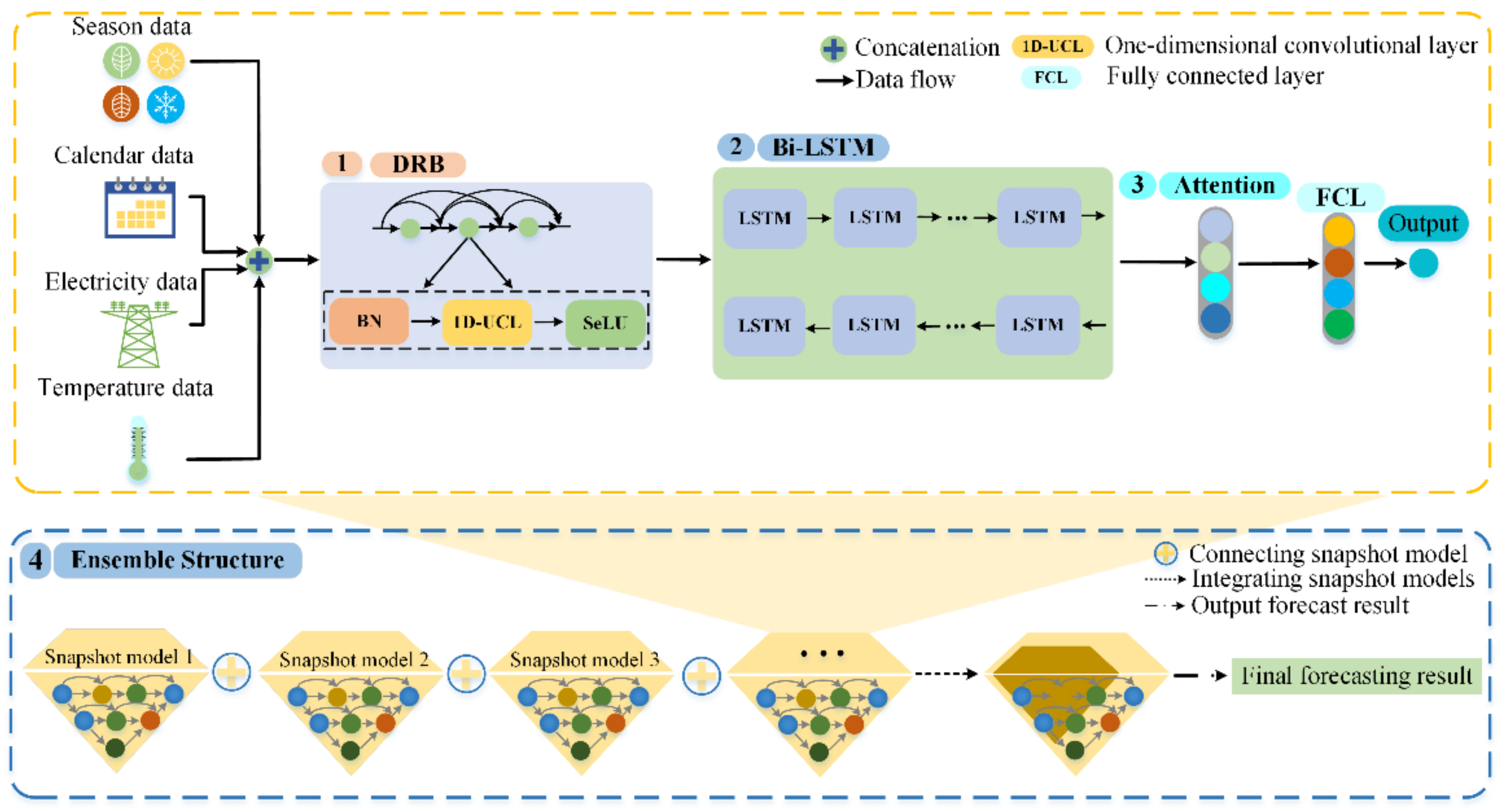
This paper proposes the innovative ensemble method combined with the DRB, Bi-LSTM, and attention mechanism for STLF, as presented in Figure 1. Specifically, the multi-scale input data are first fed into the DRB to extract the essential features that can capture the changing trend of the load series. Then, the extracted information is the input of the Bi-LSTM layer to capture the long dependency in data. The adopted attention mechanism can assign various weights to the hidden state of Bi-LSTM and focus on the crucial factors. Finally, the proposed method can ensemble multiple snapshots by the virtue of the two-stage ensemble thinking. The model obtains the final results after averaging all snapshots’ outputs.

2.2. Densely Residual Block

The existing methods usually used FCN and one-dimensional convolutional neural network (1D-CNN) for STLF [34]. However, the above methods still encounter some problems. For example, STLF models based on the FCN usually comprise many parameters. Thus, it often suffers from over-fitting and gradient disappearance. Moreover, the 1D-CNN demands that the extracted data are invariant. However, the multi-scale electricity data are virtually space-variant [25].

Therefore, the paper designs a novel densely residual block (DRB) by integrating the residual fashion and one-dimensional unshared convolutional layer, as presented in Figure 2. The designed DRB allows the model to relieve the problems caused by FCN and 1D-CNN. Compared with FCN, the DRB does not encounter over-fitting with fewer parameters. Unlike 1D-CNNs, the DRB can share the corresponding convolutional kernel parameters in different convolutional areas, as the UCNN does not require space invariance for the input variables. Specifically, this section details the implementational process of the DRB. The dataset is first expressed as follows:

$$A={\left\{\left.{\mathrm{x}}_{\mathrm{i}},{\mathrm{y}}_{\mathrm{i}}\right\}\right.}_{t=l}^n$$

(1)

where ${\mathrm{x}}_{\mathrm{i}}$ is the $l\mathrm{t}\mathrm{h}$ input data and ${\mathrm{y}}_{\mathrm{i}}$ represents the target value. The output value of 1D-UCNN converges to ${\mathrm{y}}_{\mathrm{i}}$ after a few training iterations. The region with the blue border is the feature map, as presented in Figure 3. In addition, the three squares marked in different colors can represent the various weight parameters. Specifically, the $i\mathrm{t}\mathrm{h}$ hidden layer’s feature extraction process is detailed as follows:

$$p_t^i=Z\left(h_t^{i-1}\right)$$

(2)

where $h_t^{i-1}$ is the $t\mathrm{t}\mathrm{h}$ convolutional region at $\left(i-1\right)\mathrm{t}\mathrm{h}$ layer and $p_t^i$ denotes the corresponding output value. $Z$($·$) represents the unshared convolutional operator. In addition, the different convolution areas’ outputs are concatenated as the innovative feature. It is regarded as the convolution area for the following operation.

Note that the DRB integrates the 1D-UCNN layer and residual structure to improve the network’s forecasting performance. The added shortcut connections help the related gradient data back-propagate. Specifically, the output value of the $i\mathrm{t}\mathrm{h}$ hidden layer is detailed as follows:

$$p_t^i=Z\left(h_t^{i-1}\right)+h_t^{i-1}+h_t^{i-2}$$

(3)

The DRB framework is constructed, as presented in Figure 2. Moreover, the DRB is an essential component of the proposed method. The reason is that the DBR has the ability to capture the vital features from the load data.

2.3. Bidirectional Long Short-Term Memory (Bi-LSTM)

Though the traditional methods can effectively learn the change trend of the time series data, the models cannot produce satisfactory forecast results. The reason is that they often present complicated random features. Therefore, the LSTM is an improved architecture of recurrent neural network (RNN) to overcome the above problem [31].

The memory cell of the LSTM block comprises input gate, forgetting gate, output gate, and cell state. They can help cells to capture the long dependence characteristics. The computing formula of the LSTM block is as follows:

$$i_t=\sigma \left(w_i{h}_{t-1}+w_i{x}_t+b_i\right)$$

(4)

$$f_t=\sigma \left(w_f{h}_{t-1}+w_f{x}_t+b_f\right)$$

(5)

$$o_t=\sigma \left(w_o{h}_{t-1}+w_o{x}_t+b_o\right)$$

(6)

$$\widetilde{c_t} =tanh \left(w_c{h}_{t-1}+w_c{x}_t+b_c\right)$$

(7)

$$c_t=f_t\circ c_{t-1}+i_t\circ \widetilde{c_t}$$

(8)

$$h_t=o_t\circ tanh\left(c_t\right)$$

(9)

where $\sigma$ denotes the sigmoid activation function. $i_t$; $f_t$, and $o_t$ represent the output of input gate, forget gate, and output gate, respectively. $\widetilde{c_t}$ represents the cell state’s output value. In addition, $c_t$ is the cell’s output. $h_{t-1}$ is the hidden state at time step $t-1$. In addition, $x_t$ and $h_t$ are input and output at time step t, respectively.$w$ and $b$ denote the weight matric and bias, respectively. Specifically, $w$ and $b$ are updated according to the difference between the calculated output and input.

The traditional LSTM only learns the previous context of the input data, limiting the model generalization. Thus, the Bi-LSTM is adopted to relieve the above problem. Specifically, the Bi-LSTM learns the sequence data in opposite directions simultaneously by the forward layer and backward layer. The computing formula of the Bi-LSTM layers is as follows:

$${\overrightarrow{i}}_t=\sigma \left({\overrightarrow{w}}_i{\overrightarrow{h}}_{t-1}+{\overrightarrow{w}}_i{\overrightarrow{x}}_t+{\overrightarrow{b}}_i\right)$$

(10)

$${\overrightarrow{f}}_t=\sigma \left({\overrightarrow{w}}_f{\overrightarrow{h}}_{t-1}+{\overrightarrow{w}}_f{\overrightarrow{x}}_t+{\overrightarrow{b}}_f\right)$$

(11)

$${\overrightarrow{o}}_t=\sigma \left({\overrightarrow{w}}_o{\overrightarrow{h}}_{t-1}+{\overrightarrow{w}}_o{\overrightarrow{x}}_t+{\overrightarrow{b}}_o\right)$$

(12)

$$\overrightarrow{\widetilde{c_t} } =tanh \left({\overrightarrow{w}}_c{\overrightarrow{h}}_{t-1}+{\overrightarrow{w}}_c{\overrightarrow{x}}_t+{\overrightarrow{b}}_c\right)$$

(13)

$$\overrightarrow{c_t}=\overrightarrow{f_t}\circ {\overrightarrow{c}}_{t-1}+\overrightarrow{i_t}\circ \overrightarrow{\widetilde{c_t} }$$

(14)

$${\overrightarrow{h}}_t={\overrightarrow{o}}_t\circ tanh\left(\overrightarrow{c_t}\right)$$

(15)

$${\overleftarrow{i}}_t=\sigma \left({\overleftarrow{w}}_i{\overleftarrow{h}}_{t-1}+{\overleftarrow{w}}_i{\overleftarrow{x}}_t+{\overleftarrow{b}}_i\right)$$

(16)

$${\overleftarrow{f}}_t=\sigma \left({\overleftarrow{w}}_f{\overleftarrow{h}}_{t-1}+{\overleftarrow{w}}_f{\overleftarrow{x}}_t+{\overleftarrow{b}}_f\right)$$

(17)

$${\overleftarrow{o}}_t=\sigma \left({\overleftarrow{w}}_o{\overleftarrow{h}}_{t-1}+{\overleftarrow{w}}_o{\overleftarrow{x}}_t+{\overleftarrow{b}}_o\right)$$

(18)

$$\overleftarrow{\widetilde{c_t}}=tanh \left({\overleftarrow{w}}_c{\overleftarrow{h}}_{t-1}+{\overleftarrow{w}}_c{\overleftarrow{x}}_t+{\overleftarrow{b}}_c\right)$$

(19)

$${\overleftarrow{c}}_t=\overleftarrow{f_t}\circ {\overleftarrow{c}}_{t-1}+{\overleftarrow{i}}_t\circ \overleftarrow{\widetilde{c_t}}$$

(20)

$${\overleftarrow{h}}_t={\overleftarrow{o}}_t\circ tanh ({\overleftarrow{c}}_t)$$

(21)

$$h_t={\overrightarrow{h}}_t\circ {\overleftarrow{h}}_t$$

(22)

where the opposite-oriented arrows represent the learning process of the forward and backward, respectively. $h_t$ denotes the final hidden status at time step t, which is calculated by computing ${\overrightarrow{h}}_t$ and ${\overleftarrow{h}}_{\mathrm{t}}$ Thus, Bi-LSTM has the ability to efficiently learn the crucial features from input series and produce the final output.

2.4. Attention Mechanism

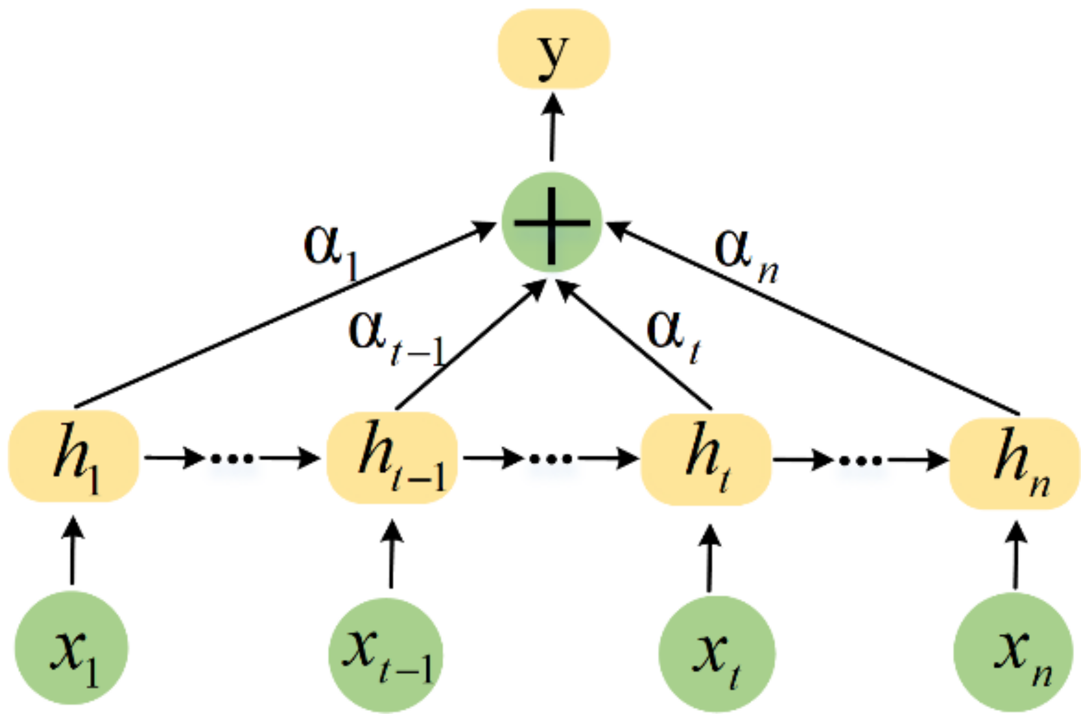
The attention mechanism [37] is an effective method to allocate the resource, and its operation process is similar to the human brain’s attention. The crucial idea is to ignore the irrelevant information and only focus on the required information. Specifically, the hidden layer status is determined by the various weight, thereby efficiently improving the forecasting performance. The attention mechanism is presented in Figure 4.

As indicated in Figure 4, $x_t$ is the Bi-LSTM network’s input data. $h_t$ denotes the output value of hidden layers with input data through the Bi-LSTM. ${\alpha }_t$ means the attention probability distribution value concerning the Bi-LSTM hidden layer.$y$ is the output value of the proposed method after adopting the attention mechanism.

2.5. Ensemble Structure

The ensemble model can produce more accurate forecast results compared with the single ones [29,30,31]. In addition, experimental results show that ensemble thinking helps the model improve forecasting performance. Therefore, this paper proposes two-stage ensemble thinking in this paper.

The proposed model applied the adaptive moment estimate (Adam) [38] to optimize the method in the first stage, as the Adam can effectively help the model adjust the learning rate in different training stages. Specifically, the model adopts a larger learning rate at the beginning stage and it can help the model speed to the best solution. Then, a lower learning rate can promote training stability and prevent skipping the best solution. Next, the model saves a few snapshots following the proposed ensemble method in [39]. Specifically, when the proposed method runs to the snapshot point, the model saves the snapshot. Then, the model continues running until the following snapshot point. In the second stage, it is worth noting that the model regards the number of snapshots as the hyper-parameter, and its confirmation process is detailed in Section 3. The above ensemble thinking can ensemble accurate snapshot models while reducing the training period. Finally, the model averages the output of all the snapshots, and the average value is the final forecast.

2.6. Forecasting Evaluation

The performance metrics need to be adopted to evaluate the generalization ability of the models. Concretely, the metrics include mean absolute error (MAE), mean absolute percentage error (MAPE), and root-mean-squared error (RMSE), which are shown as follows:

$$\mathrm{MAE}=\frac{1}{Num}{\displaystyle \sum _{i=1}^{Num}\left|V_i-F_i\right|}$$

(23)

$$\mathrm{MAPE}=\frac{1}{Num}{\displaystyle \sum _{i=1}^{Num}\frac{\left|V_i-F_i\right|}{V_i}}\times 100\%$$

(24)

$$\mathrm{RMSE}=\sqrt{\frac{1}{Num}{\displaystyle \sum _{i=1}^{Num}{(V_i-F_i)}^2}}$$

(25)

where $V_i$ is the actual load value and $F_i$ is the forecasted value. In addition, Num is the number of the testing set.

3. Experiment Results

3.1. Test Settings

The numerical experiments of STLF are conducted on two utility-scale datasets to evaluate the model generalization. The proposed model is implemented with Keras 2.2 and TensorFlow 2.1 in the Python 3.7 environment.

The datasets from Australia and North America are used to test the forecasting accuracy of the models. Specifically, the training set of the Australian dataset is from 1 January 2011 to 31 December 2015, and the testing set is from 1 January 2016 to 31 December 2016. The North American dataset spans from 1 January 1988 to 12 October 1992, covering a total of 46 months. The data of the first 36 months are applied to train, and the data of the remaining 10 months are applied to test. The input feature consists of electricity load data, temperature data, and calendar data, as shown in

Table 1. Input variables for the load forecast of the ith hour.

Symbol	Description of the Inputs
feature1	Electricity load of recent 24 h before the ith hour of the forecasted day
feature2	Electricity load of the ith hour on the days that are 1, 2, and 3 months before the forecasted day
feature3	Electricity load of the ith hour on the days that are 1, 2, and 3 weeks before the forecasted day
feature4	Electricity load of the ith hour within a week before the forecasted day
feature5	The average value of feature2
feature6	The average value of feature3
feature7	The average value of feature4
feature8	Temperature of the ith hour on the days that are 1, 2, and 3 months before the forecasted day
feature9	Temperature of the ith hour on the days that are 1, 2, and 3 weeks before the forecasted day
feature10	Temperature of the ith hour within a week before the forecasted day
feature11	Temperature of the ith hour
feature12	The average value of feature8
feature13	The average value of feature9
feature14	The average value of feature10
feature15	One-hot encoding for season, weekend, and holiday

. The number of input features is 15. Specifically, the size of the corresponding dimension is 66. In addition, we use the same input data in the training set and testing data for a fair comparison. In addition, the benchmark methods are used for comparison with the proposed method. Note that the load and temperature in the past 24 h are the input of the benchmark methods to forecast the load on the following day, and the models’ parameters are summarized as follows:

(1)

Proposed model: The proposed ensemble model consists of five snapshots. Specifically, each snapshot comprises the DRB and Bi-LSTM based on the attention mechanism. The number of the unshared convolutional filter is 8, and the number of its kernel is 1. In addition, the Bi-LSTM has two hidden layers, and the hidden units’ size is set to 8/8. The number of the two fully-connected layers’ neurons is set to 10/1.

(2)

CNN: The model comprises two convolutional layers and three fully-connected layers. Moreover, the convolutional filter’s size is 32, and the number of its kernel is 1. The size of the three fully-connected layers’ neurons is set to 10/10/1.

(3)

LSTM: The model has two hidden layers, and the hidden units’ size is set to 16/16.

(4)

PCL [33]: The CNN and LSTM networks are implemented by two different paths without correlation in both paths. The input data are first fed to CNN and LSTM path to extract the essential spatiotemporal features in load series. Then, the extracted information is the input of the fully-connected layers and dropout layers to produce the final output.

(5)

MCL [36]: Different from PCL [33], the MCL [36] adopts the three 1D-CNNs to extract the features from historical load, weather data, and calendar data, respectively, improving the ability of the feature extraction.

(6)

DCRN [31]: The model designs an innovative residual network combined with 1D-CNNs and Bi-LSTM layers. The advanced residual structure can help the model overcome the over-fitting and fully take advantage of the deep learning method.

3.2. Results of the Australian Dataset

This section first evaluates the influence of the various hyperparameters on model generalization. Specifically, the hyperparameter is determined by the number of snapshot models taken in the model’s training stage. In addition, the performance comparison of the different amounts of the snapshot models is presented in

Table 2. The performance comparison with various hyperparameters of the Australian dataset.

Snapshot	MAPE (%)	MAE (MWh)	RMSE (MWh)
2	6.76	548.6	854.6
3	6.68	541.9	851.4
4	6.51	528.7	820.5
5	6.42	515.7	812.6
6	6.64	539.2	850.7

. It is observed that the model can produce the lowest performance error while integrating five snapshots. Thus, the proposed ensemble model is composed of five snapshots in this paper.

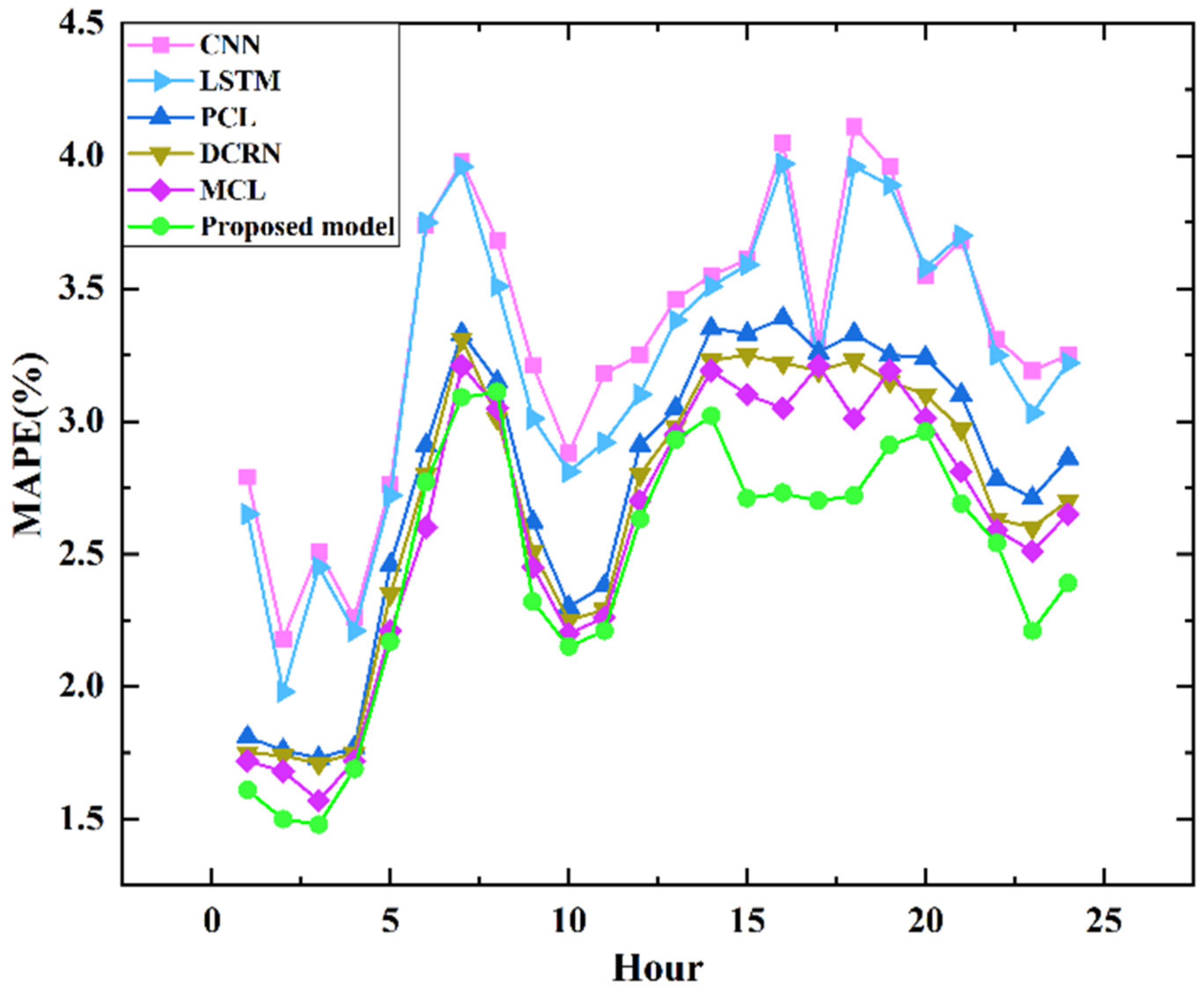
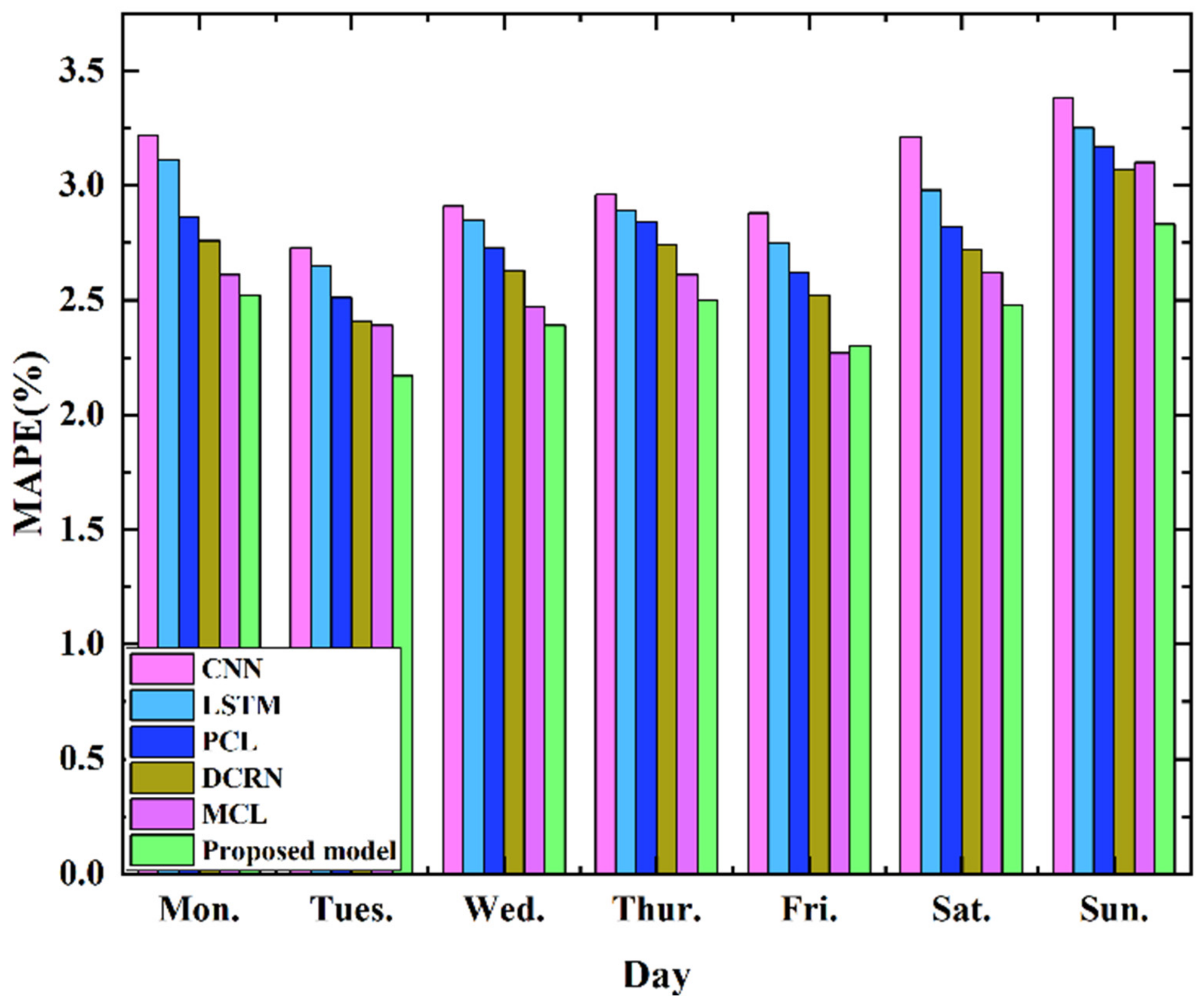
The load forecast results of the benchmark methods and the proposed method are presented in Figure 5. The proposed method can obtain the best accurate forecast result at 1 am, and the reason is that the actual load data concerning the previous 24 h is the input of the method. It is observed from Figure 5 that the forecast deviation of the proposed model is maximum at 8 am, and the MAPE is 3.11%. In addition, the MAPE of the proposed method is higher compared to DCRN [31] and MCL [36] at only 6 am. The results demonstrate that the proposed model produces better forecasting accuracy compared to the other benchmark methods in the most hours of one day. In addition, forecasted results of the proposed method and benchmark ones within a week are presented in Figure 6. The comparison indicates that the proposed method obtains the most accurate results compared to the benchmark methods.

The comparative results of the proposed model and the benchmark ones are presented in

Table 3. Performance comparison between MAPEs, MAEs, and RMSEs on the Australian dataset during 2016.

Model	MAPE (%)	MAE (MWh)	RMSE (MWh)
CNN	3.52	275.6	414.5
LSTM	3.31	255.9	401.3
PCL [33]	3.01	225.7	392.1
DCRN [31]	2.72	210.5	354.5
MCL [36]	2.69	205.9	346.2
Proposed model	2.53	194.8	343.3

. Specifically, hybrid methods such as MCL [36], DCRN [31], and PCL [33] can produce more accurate forecast results than CNN and LSTM models. The reason is that the hybrid model can simultaneously capture the spatial features and time dependence in load series. Thus, the forecasting performance is improved. Note that the forecasting accuracy of the MCL [36] is higher than PCL [33] and DCRN [31]. The reason is that the series structure based on CNN and LSTM has better learning efficiency than the parallel structure. In addition, the MAPE value of the proposed model obtains a decline of 5.94%, and the corresponding MAE value decreases by 5.39%, RMSE value decreases by 0.83% than MCL [36], and the above performance indexes are the minimum values of six models. Thus, the results show that the densely residual block (DRB) of the proposed model can effectively extract the essential characteristics of load, temperature, and calendar data. Moreover, it also demonstrates that the introduced attention mechanism can improve model generalization.

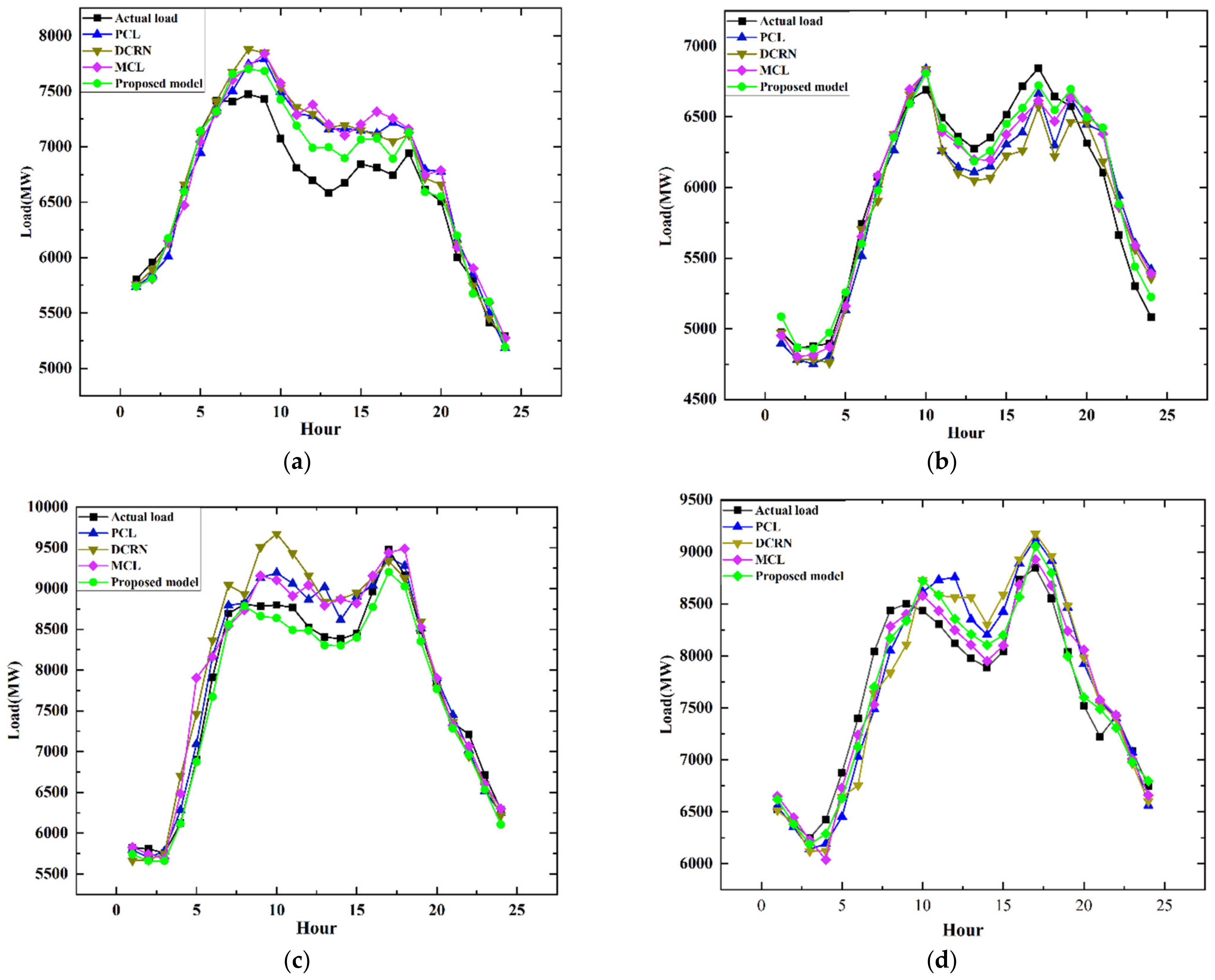
The performance comparison of the proposed model and benchmark between seasons is further implemented. The forecast results of the models in different seasons are shown in Figure 7 and

Table 4. Performance comparison between MAPEs, RMSEs, and MAEs in spring.

Model	MAPE (%)	MAE (MWh)	RMSE (MWh)
CNN	3.63	286.4	479.5
LSTM	3.59	277.2	471.1
PCL [33]	3.47	260.6	462.6
DCRN [31]	3.41	257.8	457.5
MCL [36]	3.31	251.8	449.2
Proposed model	3.23	244.5	447.9

,

Table 5. Performance comparison between MAPEs, RMSEs, and MAEs in summer.

Model	MAPE (%)	MAE (MWh)	RMSE (MWh)
CNN	2.81	207.3	327.1
LSTM	2.52	183.5	319.3
PCL [33]	2.24	167.3	284.8
DCRN [31]	2.11	151.2	257.7
MCL [36]	1.98	144.9	251.9
Proposed model	1.91	141.6	249.3

,

Table 6. Performance comparison between MAPEs, RMSEs, and MAEs in fall.

Model	MAPE (%)	MAE (MWh)	RMSE (MWh)
CNN	3.41	277.4	430.1
LSTM	3.19	256.7	408.3
PCL [33]	2.38	190.3	310.4
DCRN [31]	2.37	187.6	291.1
MCL [36]	2.21	174.8	256.6
Proposed model	1.98	159.2	262.1

and

Table 7. Performance comparison between MAPEs, RMSEs, and MAEs in winter.

Model	MAPE (%)	MAE (MWh)	RMSE (MWh)
CNN	4.62	414.5	563.4
LSTM	4.29	379.8	517.8
PCL [33]	4.27	386.3	653.1
DCRN [31]	3.33	288.9	432.8
MCL [36]	3.12	255.4	389.1
Proposed model	2.94	239.7	402.5

. Specifically, the proposed model can obtain the best forecast result, MAPE is 3.23%, MAE is 244.5, and RMSE is 447.9 in spring. In addition, it can be seen from Table 3 that the PCL [33] achieves satisfactory forecasting accuracy. The MAPE value of the proposed model has a decline of 2.41%, and its MAE value decreases by 2.89%, RMSE decreases by 0.28% compared to the PCL [33]. Though both methods have large forecasting error from 9 am to 12 am, the forecast result of the proposed framework is more similar to the load trend.

In summer, the forecasting accuracy of the proposed model is best, with MAPE of 1.91%, MAE of 141.6, and RMSE of 249.3, as shown in Table 5. The performance index is a decrease in MAPE by 3.53% than PCL [33], which has the second smallest forecasting error, 2.27% lower in MAE than MCL [36]. The performance comparison of the proposed method, PCL [33], and MCL [36] is presented in Figure 7b. Specifically, the forecasting errors of PCL [33] and MCL [36] are large at 3 pm. The electricity load rises significantly in the afternoon, and the methods present a similar forecast load. Nevertheless, the proposed method can produce more accurate forecast results than PCL [33] and MCL [36].

In the fall, the proposed model is excellent, with an MAE of 157.2 and RMSE of 262.1, but MCL [36] produces the lowest MAPE of 256.6, as presented in Table 6. The MAPE value of the proposed method is decreased by 1.04%, and MAE is decreased by 8.92% in percentage comparison. However, the RMSE of PCL [33] is decreased by 2.09% than the proposed method. The performance comparison of the two models is presented in Figure 7c. Both models have no significant errors in forecasting the maximum load. However, the forecasting error of the proposed model is small in forecasting the minimum load. Thus, the proposed model can produce better accuracy in forecasting the lowest load.

In the winter, the proposed model has the best forecast results, as presented in Table 7. The MAPE of the proposed method is 2.94% and its MAE is 402.5. However, the MCL [36] has the lowest RMSE of 255.4. It is observed from Figure 7d that the range of the electricity load fluctuation is large in low-temperature conditions. Thus, it is challenging to forecast the maximum and minimum electricity loads. Though the proposed model has the best forecasting performance during winter, it still needs to improve. In summary, the results demonstrate that the proposed model can achieve satisfactory forecasting efficiency based on the performance comparison of the models within the year.

3.3. Results of the North American Dataset

The forecast results of the proposed model and benchmark are shown in Figure 8. It is worth noting that the MAPE on the North American dataset is higher than that on the Australian dataset. The reason is that the North American dataset is relatively unstable and has fewer samples. It is observed from Figure 8 that the proposed method obtains the best performance at 1 am and the reason is that the input data concerning the previous 24 h are all actual load. The proposed model has the maximum deviation at 5 pm, and the MAPE is 4.03%. Moreover, the MAPE value of the proposed method is higher compared with DCRN [31] and MCL [36] only at 6 am. Thus, the results demonstrate that the proposed model obtains better forecasting accuracy compared to the other methods for most hours.

The comparison of the proposed method and benchmark methods for the North American dataset is presented in

Table 8. Performance comparison between MAPEs, MAEs, and RMSEs on the North American dataset during 1991.

Model	MAPE (%)	MAE (MWh)	RMSE (MWh)
CNN	3.91	472.7	739.6
LSTM	3.87	453.3	699.5
PCL [33]	3.58	444.1	659.6
DCRN [31]	3.41	435.1	634.8
MCL [36]	3.26	424.1	600.5
Proposed model	3.15	417.2	583.1

. Compared with MCL [36], the MAPE value of the proposed method has a large decline of 3.37%, the corresponding MAE value decreases by 1.65%, and the RMSE value decreases by 2.81%. In addition, the performance indexes of the proposed method are the minimum in the benchmark models. It is observed from Table 8 that the proposed model outperforms existing methods in forecasting performance. The reason is that the attention mechanism can effectively improve the forecasting performance and fitting effect of the Bi-LSTM layers. In addition, the designed DRB can effectively capture the multi-scale features that affect the load change from input data. Therefore, the forecasting performance of the proposed method is improved.

In this section, comparative simulations are implemented to test the effectiveness of the different modules used in the proposed model. Concretely, this section compares the forecasting performance of the whole proposed model, the proposed model removing densely residual block (PMrDRB), the proposed model removing attention mechanism (PMrAM), and the proposed model removing Bi-LSTM (PMrBL). In addition, the evaluations are implemented on three performance indexes including MAPE, MAE, and RMSE. The comparative results are presented in

Table 9. Performance validation of the modules in the proposed model.

Models	MAPE (%)	MAE (MWh)	RMSE (MWh)
PMrDRB	3.57	461.8	646.5
PMrAM	3.35	440.9	620.3
PMrBL	3.28	437.8	615.7
Proposed model	3.15	417.2	583.1

.

It can be observed that the densely residual block can contribute most to the forecasting performance. Specifically, the MAPE value has a large decline of 11.7%, the corresponding MAE value decreases by 9.5%, and the RMSE value decreases by 9.8%. The improvement in forecasting performance can be attributed to the unshared convolutional neural network and residual structure. The model can effectively extract the crucial features to promote forecasting accuracy. It can be seen from the 2nd and 4th rows that the Bi-LSTM layers behave well in reducing the MAPE value. It decreases by 3.96%. In addition, according to the 3rd and 4th rows of Table 9, the attention mechanism also promotes the generalization ability of the model. The MAPE value is reduced by 5.97%. Thus, the improved performance contributed by the different modules is verified.

4. Conclusions

Short-term load forecasting is essential for the sustainable operation of the power system, and it has the ability to overcome the problem caused by the lack of electricity supply. Thus, the study proposes an innovative STLF method that consists of the DRB, Bi-LSTM layers, and attention mechanism. Specifically, the DRB based on the unshared convolutional neural network can relieve the limitation of the CNN-based models without the requirement of space invariance. It can extract the crucial features from input data. The paper reports the forecast results of the proposed model on two datasets. Experimental results demonstrate that the proposed model obtains more accurate forecast results than the mainstream schemes.

This paper still has some limitations to improve. For instance, the proposed model of this paper is only used for deterministic load forecasting, which cannot show the uncertainty of the electricity load. Interval forecasting and probabilistic forecasting need to be implemented to relieve the above problem. In future work, the advanced optimization algorithm can be adopted to tune the parameters of the proposed method. External factors, such as wind speed and humidity, can also be introduced into the model to boost model generalization.

References

1. Wu, L.; Shahidehpour, M. A hybrid model for day-ahead price forecasting. IEEE Trans. Power Syst. 2010, 25, 519–1530. [Google Scholar]
2. Abedinia, O.; Amjady, N.; Zareipour, H. A new feature selection technique for load and price forecast of electrical power systems. IEEE Trans. Power Syst. 2017, 32, 62–74. [Google Scholar] [CrossRef]
3. Borges, C.E.; Penya, Y.K.; Fernandez, I. Evaluating combined load forecasting in large power systems and smart grids. IEEE Trans. Ind. Informat. 2013, 9, 1570–1577. [Google Scholar] [CrossRef]
4. Singh, P.; Dwivedi, P.; Kant, V. A hybrid method based on neural network and improved environmental adaptation method using controlled Gaussian mutation with real parameter for short-term load forecasting. Energy 2019, 174, 460–477. [Google Scholar] [CrossRef]
5. Lusis, K.R.; Andrew, L.; Liebman, A. Short-term residential load forecasting: Impact of calendar effects and forecast granularity. Appl. Energy 2017, 205, 654–669. [Google Scholar] [CrossRef]
6. Hippert, H.S.; Pedreira, C.E.; Souza, R.C. Neural networks for short-term load forecasting: A review and evaluation. IEEE Trans. Power Syst. 2001, 16, 44–55. [Google Scholar] [CrossRef]
7. Kong, W.; Dong, Z.Y.; Jia, Y.; Hill, D.; Xu, Y.; Zhang, Y. Short-term residential load forecasting based on LSTM recurrent neural network. IEEE Trans. Smart Grid. 2019, 10, 841–851. [Google Scholar] [CrossRef]
8. Mbamalu, G.; Hawary, M. Load forecasting via suboptimal seasonal autoregressive models and iteratively reweighted least squares estimation. IEEE Trans. Power Syst. 1993, 8, 343–348. [Google Scholar] [CrossRef]
9. Zhang, H.; Zhu, T. Stacking model for photovoltaic-power-generation prediction. Sustainability 2022, 14, 5669. [Google Scholar] [CrossRef]
10. Abdellatif, A.; Mubrak, H.; Ahmad, S.; Ahmed, T.; Shafiullah, G.M.; Hammoudeh, A.; Abdellatef, H.; Rahman, M.M.; Gheni, H.M. Forecasting photovoltaic power generation with a stacking ensemble model. Sustainability 2022, 14, 11083. [Google Scholar] [CrossRef]
11. Lateko, A.A.H.; Yang, H.T.; Huang, C.M.; Aprillia, H.; Hsu, C.Y.; Zhong, J.L.; Phuong, N.H. Stacking ensemble method with the RNN meta-learner for short-term PV power forecasting. Energies 2021, 14, 4733. [Google Scholar] [CrossRef]
12. Zhang, X.; Chan, K.W.; Li, H.; Wang, H.; Wang, G. Deep learning based probabilistic forecasting of electric vehicle charging load with a novel queuing model. IEEE Trans. Cybern. 2021, 6, 3157–3170. [Google Scholar] [CrossRef] [PubMed]
13. Song, K.B.; Baek, Y.S.; Hong, D.H.; Jang, G. Short-term load forecasting for the holidays using fuzzy linear regression method. IEEE Trans. Power Syst. 2005, 20, 96–101. [Google Scholar] [CrossRef]
14. López, J.C.; Rider, M.J.; Wu, Q. Parsimonious short-term load forecasting for optimal operation planning of electrical distribution systems. IEEE Trans. Power Syst. 2019, 34, 1427–1437. [Google Scholar] [CrossRef] [Green Version]
15. Fan, S.; Chen, L. Short-term load forecasting based on an adaptive hybrid method. IEEE Trans. Power Syst. 2006, 21, 392–401. [Google Scholar] [CrossRef]
16. Zhang, G.; Guo, J. A novel method for hourly electricity demand forecasting. IEEE Trans. Power Syst. 2020, 35, 1351–1363. [Google Scholar] [CrossRef]
17. Singh, P.; Dwivedi, P. Integration of new evolutionary approach with artificial neural network for solving short term load forecast problem. Appl. Energy 2018, 217, 537–549. [Google Scholar] [CrossRef]
18. Quan, H.; Srinivasan, D.; Khosravi, A. Short-term load and wind power forecasting using neural network-based prediction intervals. IEEE Trans. Neural Netw. Learn Syst. 2014, 25, 303–315. [Google Scholar] [CrossRef]
19. Senjyu, T.; Takara, H.; Uezato, K.; Funabashi, T. One-hour-ahead load forecasting using neural network. IEEE Trans. Power Syst. 2002, 17, 113–118. [Google Scholar] [CrossRef]
20. Cheng, L.; Zang, H.; Xu, Y.; Wei, Z.; Sun, G. Probabilistic residential load forecasting based on micrometeorological data and customer consumption pattern. IEEE Trans. Power Syst. 2021, 36, 3762–3775. [Google Scholar] [CrossRef]
21. Arif, A.; Wang, Z.; Wang, J.; Matheret, B.; Bashualdo, H.; Zhao, D. Load modeling—A review. IEEE Trans. Smart Grid. 2018, 9, 5986–5999. [Google Scholar] [CrossRef]
22. Shao, X.; Pu, C.; Zhang, Y.; Kim, C.S. Domain fusion CNN-LSTM for short-term power consumption forecasting. IEEE Access 2020, 8, 188352–188362. [Google Scholar] [CrossRef]
23. Jiang, L.; Wang, X.; Li, W. Hybrid Multitask Multi-Information Fusion Deep Learning for Household Short-Term Load Forecasting. IEEE Trans. Smart Grid. 2021, 12, 5362–5372. [Google Scholar] [CrossRef]
24. Jalali, S.M.J.; Ahmadian, S.; Khosravi, A. A Novel Evolutionary-Based Deep Convolutional Neural Network Model for Intelligent Load Forecasting. IEEE Trans Ind. Informat. 2021, 17, 8243–8253. [Google Scholar] [CrossRef]
25. Chen, L.C.; Papandreou, G.; Kokkinos, I.; Murphy, K.; Yuille, A.L. Semantic Image Segmentation with Deep Convolutional Nets and Fully Connected. arXiv 2014, arXiv:1412.7062. [Google Scholar]
26. Dokur, E.; Erdogan, N.; Kucuksari, S. EV fleet charging load forecasting based on multiple decomposition with CEEMDAN and swarm decomposition. IEEE Access 2022, 10, 62330–62340. [Google Scholar] [CrossRef]
27. Zheng, H.; Lin, F.; Feng, X.; Chen, Y. A hybrid deep learning model with attention-based Conv-LSTM networks for short-term traffic flow prediction. IEEE Trans. Intell. Transp. Syst. 2021, 22, 6910–6920. [Google Scholar] [CrossRef]
28. Wang, S.; Wang, X.; Wang, S.; Wang, D. Bi-directional long short-term memory method based on attention mechanism and rolling update for short-term load forecasting. Electric Power Syst. Res. 2019, 109, 470–479. [Google Scholar] [CrossRef]
29. Zhao, W.; Jiao, L.; Ma, W. Superpixel-based multiple local CNN for panchromatic and multispectral image classification. IEEE Geosci. Remote Sens. Lett. 2017, 55, 4141–4156. [Google Scholar] [CrossRef]
30. Kim, T.Y.; Cho, S.B. Predicting residential energy consumption using CNN-LSTM neural networks. Energy 2019, 182, 72–81. [Google Scholar] [CrossRef]
31. Ko, M.S.; Lee, K.; Kim, J.K. Deep concatenated residual network with bidirectional LSTM for One-Hour-Ahead Wind Power Forecasting. IEEE Trans. Sustain. Energy 2021, 12, 1321–1335. [Google Scholar] [CrossRef]
32. Yang, T.; Li, B.; Xun, Q. LSTM-attention-embedding model-based day-ahead prediction of photovoltaic power output using bayesian optimization. IEEE Access 2019, 7, 171471–171484. [Google Scholar] [CrossRef]
33. Farsi, B.; Amayri, M.; Bouguila, N.; Eicker, U. On short-term load forecasting using machine learning techniques and a novel parallel deep LSTM-CNN approach. IEEE Access 2021, 9, 31191–31212. [Google Scholar] [CrossRef]
34. Cao, Z.; Wan, C.; Zhang, Z.; Li, F.; Song, Y. Hybrid ensemble deep learning for deterministic and probabilistic low-voltage load forecasting. IEEE Trans. Power Syst. 2020, 35, 1881–1897. [Google Scholar] [CrossRef]
35. Felice, M.D.; Yao, X. Short-term load forecasting with neural network ensembles: A comparative study [application notes]. IEEE Trans Ind. Informat. 2011, 6, 47–56. [Google Scholar] [CrossRef]
36. Goh, H.H.; Liu, H.; Dai, W. Multi-convolution feature extraction and recurrent neural network dependent model for short-term load forecasting. IEEE Access 2021, 9, 118528–118540. [Google Scholar] [CrossRef]
37. Zhao, X.D.; Chen, Y.; Guo, J.; Zhao, D. A spatial temporal attention model for human trajectory prediction. IEEE CAA J. Autom. Sin. 2020, 7, 965–974. [Google Scholar] [CrossRef]
38. Kingma, D.P.; Ba, J. Adam: A method for stochastic optimization. In Proceedings of the 3rd International Conference for Learning Representations, San Diego, CA, USA, 7–9 May 2015. [Google Scholar]
39. Huang, G.; Li, Y.; Pleisse, G. Snapshot Ensembles: Train 1, Get M for Free. arXiv 2017, arXiv:1704.00109v1. [Google Scholar]
Figure 1. The proposed method including DRB, Bi-LSTM layer, attention mechanism, and ensemble structure.
Sustainability 14 16433 g001
Figure 2. Densely residual block (DRB): BN, batch normalization; 1D-UCL, one-dimensional unshared convolutional layer.
Sustainability 14 16433 g002
Figure 3. The presentation of unshared convolution. KN1, KN2, and KN3 represent convolution kernels with the various weight parameters.
Sustainability 14 16433 g003
Figure 4. Structure of attention mechanism.
Sustainability 14 16433 g004
Figure 5. Comparison of hourly MAPE values between the proposed method and the benchmark methods.
Sustainability 14 16433 g005
Figure 6. Performance comparison of MAPE values in each day per week.
Sustainability 14 16433 g006
Figure 7. Performance comparison of the forecast results during the four different seasons. (a) Spring. (b) Summer. (c) Fall. (d) Winter.
Sustainability 14 16433 g007
Figure 8. Comparison of hourly MAPE values between the proposed method and the benchmark methods.
Sustainability 14 16433 g008