Measuring Financial Sustainability and Social Adequacy of the Italian NDC Pension System under the COVID-19 Pandemic

Abstract

The COVID-19 pandemic is presently influencing the financial sustainability and the social adequacy of public pension schemes. In this paper, we measure the effects of COVID-19 on the Italian public pension system by introducing a deterministic shock due to the pandemic in the evolution of the variables mainly involved in the system’s evaluation. These variables, namely the unemployment rate, wage growth rate, inflation rate, and mortality rates, are modeled in a stochastic framework. Our results show that COVID-19 worsens the financial sustainability of the pension system in the short–medium term, while it does not appreciably affect social adequacy in the medium term. The Italian pension system already showed a social adequacy problem before 2020, which the pandemic does not further deteriorate essentially.

1. Introduction

The World Health Organization [1] declared the coronavirus disease (COVID-19) outbreak a pandemic in early March 2020. Following this declaration, many countries worldwide put in place restrictive actions to contrast the virus spread. These actions inflicted by governments have limited the contagion expansion and reduced the number of deaths, but otherwise, they have severely affected commercial enterprises. Many persons have experienced a relevant lowering in income, experiencing a reduction or interruption in wages due to the temporary lock of labor activities. Declining sales and production shutdowns determined income losses for several firms.

The pandemic crisis is also affecting public and private pension systems, which have already been heavily weakened by the Global Financial Crisis of 2008–2009. A study of the International Monetary Fund [2] argues that the limitations of economic activity due to COVID-19 are influencing the labor market by reducing employment and stagnating or reducing real wages. Therefore, national and occupational retirement systems are experiencing a reduction in contributions paid. Workers may not be able to meet their contractual obligations by not paying contributions and thus reducing the income of the pension system.

The economic slowdown due to the pandemic could produce certain groups of near-retirees to experience significant and permanent decreases in their Social Security retirement benefits. Ref. [3] suggests several methods by which policymakers could enact changes to the pension formula to contrast these benefit reductions. Moreover, many workers take advantage of early retirement payments when they can no longer use unemployment benefits. Ref. [4] provides an overview of the measures put in place in the OECD and selected non-OECD countries to cope with the crisis and having an impact on the public pension system: some countries have allowed a temporary reduction or suspension of contributions paid to social security pension schemes; some others temporarily allowed accruing pension entitlements on the full wage (Canada) or accruing full pension entitlements by including the lost work hours contributions (Germany). In other countries (e.g., Australia, Canada, Israel, New Zealand), governments introduced measures to support low-income retirees (generally increasing their pension benefits), while France has suspended the ongoing reforms [5]. These actions raise the uncertainty of the state’s budget and might worsen the government’s ability to pay the pension benefits it promised.

Regarding occupational pension plans, the financial crisis following the COVID-19 pandemic is decreasing the investment gains that are a source of contribution in funded pension plans. Lower returns shorten their asset values, enhancing pension plans’ fiscal risk. Moreover, persisting low-interest rates reduces the discount rate used to determine the present value of liabilities in Defined Benefit (DB) schemes, increasing their liabilities [6].

The extent of the financial consequences on pension plans indeed depends on both the plan’s pre-crisis financial situation and the plan’s type. In DB schemes, the risk of resources being insufficient to cover retirement benefits obligations is borne by underwriters, whereas in defined contribution (DC) schemes, such a risk is borne by members. The first data on DB pension plans, both state and occupational, show much higher levels of underfunding than before as a consequence of the financial market shock [7]. DC schemes also suffered the brunt of the 2020 financial market shock as well as the consequences of unemployment and the reduction in GDP, even if, in this case, the consequences are paid by the beneficiaries. In DC pension funds, the reduction in asset value and the early withdrawal due to the COVID-19 pandemic will probably produce fewer future benefits and the risk of poverty for funds’ participants [2]. On the other hand, the crisis might offer an opportunity to change priorities in reform processes and address the problem of pension benefits adequacy in an economic context characterized by recession and difficulties in the labor market [8] but taking on a holistic framework that encloses the interaction between pension system purposes and constraints [9].

The deterioration in the economic conditions and in the labor market due to the COVID-19 pandemic (the unemployment rate as a percentage of the labor market in the Euro area is expected to rise from 8.3% in 2020 to 9.4% in 2021 and 8.9% in 2022 [10]) may jeopardize the financial sustainability of pension systems in the short to medium term. Moreover, changed health conditions and increased mortality at old age can have an opposite influence. Measuring this impact, with the pandemic still underway, is complex, but some authors argue that the long-term impacts of mortality due to COVID-19 will be low [11,12].

With the reforms of 1995 and 2011, the Italian pension system gradually switched from Defined Benefit to Notional Defined Contribution (NDC). The main appealing feature of an NDC is the individual actuarial fairness that directly links contributions to pension benefits and the long-term financial sustainability favored by a Defined Contribution (DC) nature [13]. Moreover, at the macro level, they should guarantee intergenerational equity and financial sustainability. These objectives are achieved thanks to the following characteristics [14]:

• The presence of a fixed contribution rate that stabilizes the weight of pension expenditure on gross domestic product (GDP) between generations;
• The recognition of a rate of return that is adjusted periodically to ensure the financial sustainability of the system;
• The link between the level of initial pension and the residual life expectancy at retirement, which limits the negative effect of longevity risk on the pension balance;
• The recognition of an economic incentive to postpone the moment of retirement by applying an actuarially fair annuity rate.

This system is balanced when the economic and demographic conditions are constant (steady state); however, longevity improvements, aging populations, and fertility decreases, as well as worse economic and labor conditions, compromise the financial sustainability and the guarantee of adequate (in terms of living standard) pensions to retirees.

We address the question of whether, due to the COVID-19 pandemic, future developments in contributions and benefits will lead to liquidity problems (benefits in excess of contributions in the short term) or solvency issue (imbalance between the present value of benefits and the present value of contributions) to the Italian NDC pension system. Moreover, we inquire whether future retirees would receive enough pension benefits to maintain basic living standards. In other words, our objective is to analyze the effects of the pandemic on the financial sustainability and social adequacy of the pension benefits of the Italian pension system. We consider “financial sustainability” from the policymaker’s perspective. Meanwhile, we refer to “social adequacy” from the retirees’ perspective, addressing the question of whether the pension benefits would adequately support the retirees’ living standards.

Aiming to shed light on how COVID-19 might influence the main economic and demographic parameters of the Italian pension system and what would be the consequences on the financial sustainability and social adequacy of the system, we pose the following important questions. How would a mortality shock and an unemployment rate shock affect the dependency ratio? What would be the impact of a shock in the unemployment rate in the following years (especially in the short term) on the pension system’s contributions and, consequently, on the system’s financial sustainability? Shocks in the wage growth rate and the inflation rate will affect the notional rate and the accumulated notional amount. How would this affect the related benefits at retirement? Would the pension amount be socially adequate in the future?

In this paper, we have attempted to answer these questions by measuring the effect of a deterministic shock due to the COVID-19 pandemic on the values of the mortality rates, unemployment rate, wage growth rate, and inflation rate, which characterize the Italian pension system. We take the values of the shock from various governmental estimates.

To characterize the NDC pension system, we develop a stochastic model depending on a few key parameters, including the mortality rate, the wage growth rate, the inflation rate, and the unemployment rate, which are used for computing the contributions and benefits of the pension system.

We develop the numerical analysis on a long time horizon (75 years) in line with the most actuarial reports evaluating pension long-term financial sustainability. However, a mathematical model can hardly be effective in predicting a complex reality such as the dynamics of a public pension system over such a long period. Therefore, we focus on comments and discussion of the results in the short and medium term.

To the best of our knowledge, this is one of the very few academic papers investigating the effects of the pandemic on public pension systems. The literature on this topic is still poor, and there are no scientific contributions about the Italian pension system on which, instead, we focus. Ref. [15] analyzed the economic and demographic impact of COVID-19 on the Kazakhstani retirement system, highlighting how mortality, income poverty, and increase in pension costs due to the COVID-19 burden the state budget. They finally offer recommendations on supporting measures to be adopted by policymakers during the post-COVID-19 period in the pension system (e.g., exempting pensioners from paying taxes to encourage active longevity). Ref. [16] examined the revenue and expenditure side of the Romanian pension system, finding the COVID-19 economic recession will, in the short term, aggravate the financial sustainability of the public pension system. Ref. [17] developed a dynamic Monte Carlo simulation model to analyze the financial consequences of the unexpected demographic deviations caused by the COVID-19 pandemic on future pension expenditure in Poland. She found that the pandemic positively affects future pensioners that would take advantage of expected higher replacement rates at retirement. Ref. [18] studied the effect of COVID-19 on the Peruvian pension system. They found that the extra mortality due to the pandemic will lessen the system’s actuarial liabilities. This outcome is mostly driven by the savings obtained from the early deaths of retirees.

The organization of this paper is as follows. Section 2 provides the methodology. We describe the main features of the NDC system and the stochastic modeling of economic and demographic variables, introducing the pandemic shocks. Section 3 illustrates the results of a numerical application for the Italian NDC system. Section 4 provides a discussion of the results, and Section 5 concludes the paper.

2. Methodology

2.1. NDC Schemes

Our analysis focuses on the effect of COVID-19 on the social adequacy and financial sustainability of the Italian NDC system. Such a system was introduced in Italy by the Dini reform in 1995. In addition to Italy, Sweden, Latvia, and Poland have adopted an NDC system [19].

The notional rate of return, the fixed contribution rate, the retirement age, the pension indexation, and the conversion coefficient multiplying the final notional account to determine the first pension amount are the principal variables of an NDC system. The system is founded on a Pay-As-You-Go (PAYG) mechanism that uses total current contributions to finance pension benefits. The pension calculation follows a DC approach, where benefits are computed by the amount of contribution paid during the working age and the accumulated earnings through a notional rate of return on contributions. The notional amount accrued at retirement is transformed into a life annuity considering the remaining life expectancy on average. In an NDC scheme, there is no accumulation of financial assets. The word “notional” relates to the PAYG nature that requires the creation of notional accounts used to calculate the amount of pension. In Italy, the notional rate of return is set equal to the nominal GDP five-year moving average.

Despite the establishment of an NDC scheme, the population aging and the reduction of the active population are jeopardizing the financial equilibrium of the Italian NDC pension system. These conditions could compromise the financial sustainability of the system and the adequacy of future pension benefits. The impact of the COVID-19 pandemic on the economic and demographic conditions will probably result in further stress for the pension system.

In order to represent the NDC system dynamics, we follow [20], which refers to a PAYG pension scheme paying retirement benefits, disregarding survivor benefits, invalidity benefits, and withdrawals. We consider the following states: active (1), pensioner (2), dead (3), and unemployed (4). The transition probabilities between states are a function of age and time. Consequently, the eligibility for pension benefits does not depend on the years of service.

The PAYG scheme is balanced in a generic year t when annual income from contributions, $C\left(t\right)$, is equal to annual expenditure on pensions, $B\left(t\right)$. The condition $C\left(t\right)=B\left(t\right)$ can be expressed as:

$$N^1\left(t\right)·c\left(t\right)·s\left(t\right)=N^2\left(t\right)·b\left(t\right)$$

(1)

where the followingdefinitions apply:

• $N^i\left(t\right)$ is the total population in the state i at time t, and it is given by $N^i\left(t\right)={\sum }_x{N}^i(x,t)$, where $N^i(x,t)$ is the number of lives in state i at age x at time t. The latter depends on the new entrants in state i aged x in year t, $Z^i(x,t)$ and the previous-year population who have survived by time t: $N^i(x,t)=N^i(x-1,t-1)p^{ii}(x-1,t-1)+Z^i(x,t)$ for $i=1,2,3,4$, where $p^{ii}(x-1,t-1)$ is the probability for an individual aged $x-1$ in year $t-1$ to remain in state i for one year (for the equations of new entrants $Z^i(x,t)$ for $i=1,2,3$ see [20]. Regarding the unemployed, we assume that $Z^4(x,t)=Z^4\left(t\right)d_z^4(x,t)$, where $d_z^4(x,t)$ is the relative age distribution of the new unemployed and $Z^4\left(t\right)$ is the total new entrants in the unemployed state at time t. We suppose the same relative age distribution for the new unemployed population and the new actives: $d_z^4(x,t)=d_z^1(x,t)$, and $N^4\left(t\right)=\frac{\upsilon \left(t\right)}{1-\upsilon \left(t\right)}·N^1\left(t\right)$, with $N^1\left(t\right)=N^1(t-1)(1+\rho \left(t\right))$ depending on the total active population growth rate $\rho \left(t\right)$ that equally influences contributors).
• $c\left(t\right)$ is the contribution rate of the pension system at time t. Note that in an NDC system, the contribution rate is set constant over time: $c\left(t\right)=c$ for all t.
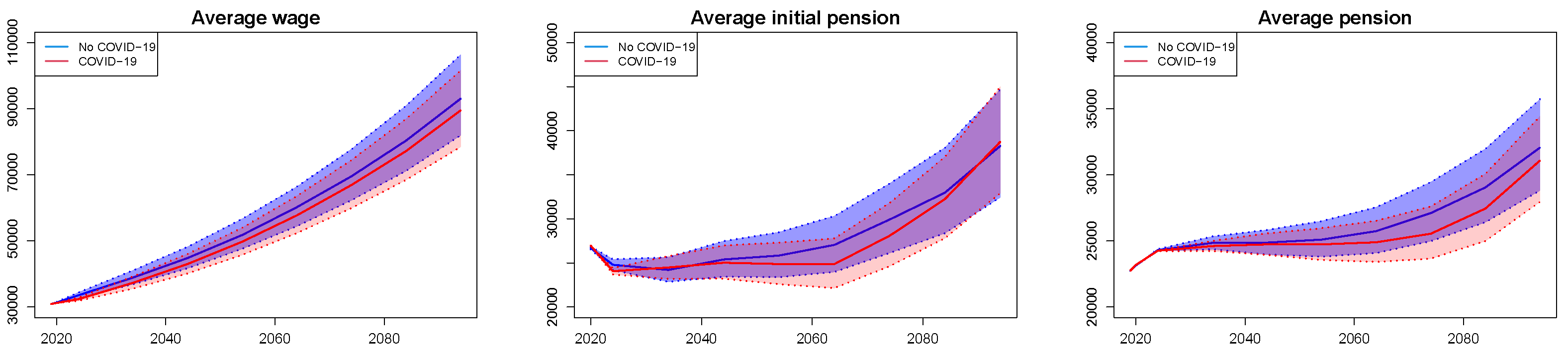
• $s\left(t\right)$ is the average wage at time t, which is given by $s\left(t\right)=\frac{S\left(t\right)}{N^1\left(t\right)}$, where $S\left(t\right)={\sum }_{x}S(x,t)$ is the total wage at time t, and $s(x,t)=s(x,t-1)\left[1+\xi \left(t\right)\right]$ is the individual wage depending on the growth rate of individual wage from $t-1$ to t, $\xi \left(t\right)$.
• $b\left(t\right)$ is the average pension paid to retirees in year t. It is given by $b\left(t\right)=\frac{B\left(t\right)}{N^2\left(t\right)}$, where $B\left(t\right)$ is the amount of total pensions paid to retirees at time t. It is given by $B\left(t\right)={\sum }_{x}B(x,t)$, where $B(x,t)$ is the total pensions paid to all retirees aged x at time t, which depends on the pension indexation rate $\lambda (t-1)$ and the total benefits paid to the new retirees in the year t, $B_z(x,t)$ ($B_z(x,t)$ is a function of the notional rate $g\left(t\right)$ that is the rate of return remunerated on the individual notional account, the expected indexation rate ${\lambda }^{*}\left(k\right)$ for $k\ge t$, and the expected rate of return, $g^{*}\left(k\right)$ for $k\ge t$ (see [20] for further details)).

We define the equilibrium contribution rate $\widehat{c}\left(t\right)$ as the contribution rate satisfying Equation (1):

$$\widehat{c}\left(t\right)=D\left(t\right)·r\left(t\right)$$

(2)

where $D\left(t\right)=\frac{N^2\left(t\right)}{N^1\left(t\right)}$ is the dependency ratio and $r\left(t\right)=\frac{b\left(t\right)}{s\left(t\right)}$ is the average replacement rate of the system in year t.

The economic dynamics and population structure evolution might threaten the stability of the PAYG pension system. While in a pure Defined Benefit-PAYG system, where benefits are fixed, the equilibrium can be restored by changing the contribution rate (for instance, Ref. [21] find the optimal contribution rate of a PAYG pension in a Nash equilibrium model to face the shrinking working population), in an NDC pension scheme, in which the contribution rate must be steady, the equilibrium is achieved by modifying (generally decreasing) the replacement rate. It can be attained by changing the notional rate that is related to the economic conditions and changes in the expected survival probabilities of pensioners, reflecting life expectancy evolution (as observed by [20], there are situations where an NDC system is not able to immediately restore the equilibrium, thus remaining vulnerable to demographic and economic shocks). Modifying the replacement rate on one side might assure the pension scheme is financially sustainable, while on the other side, it might fail to guarantee adequate benefits, lowering the living standard of beneficiaries as well as the attractiveness of the scheme for new members. In this situation, a “social sustainability” question could arise. We quantify it using the replacement rate, $r\left(t\right)$, which is the ratio between the average pension amount and the average wage of active members of the scheme.

The situation described above highlights the need, also in the case of non-funded pension systems such as the PAYG, to constitute a buffer or reserve fund that depends on the difference between income from contributions and expenditure on pensions. The reserve fund $F\left(t\right)$ at time $t\in [0,T]$ is calculated as follows:

$$F\left(t\right)=F(t-1)\left[1+g(t-1)\right]-UL\left(t\right)$$

(3)

where $UL$ represents the unfunded liabilities, $UL\left(t\right)=B\left(t\right)-C\left(t\right)$. We assume that $F\left(t\right)$’s rate of return equals the notional rate $g(t-1)$ and that, at initial time, the reserve fund is null, $F\left(0\right)=0$.

Evaluating the financial sustainability of the system requires drawing up the actuarial balance, which in PAYG systems is usually compiled by comparing the Net Present Value of the system over a long period, $NPV(0,T)$ [22]:

$$NPV(0,T)=\sum _{t=1}^{T}B\left(t\right)\prod _{h=0}^{t-1}{\left[1+g\left(h\right)\right]}^{-1}-\sum _{t=1}^{T}C\left(t\right)\prod _{h=0}^{t-1}{\left[1+g\left(h\right)\right]}^{-1}$$

(4)

Equation (4) can be expressed using the unfunded liabilities’s present value:

$$NPV(0,T)=-\sum _{t=1}^{T}UL\left(t\right)\prod _{h=0}^{t-1}{\left[1+g\left(h\right)\right]}^{-1}$$

(5)

Whether $NPV$ was non-negative in the long run ($NPV(0,T)\ge 0$), the pension system would be financially sustainable.

The system’s financial sustainability can be also measured by the annual value of the reserve fund. In this case, the system would be sustainable if $F\left(t\right)\ge 0$ in the long run.

The financial sustainability condition may be also explained using the reserve fund. Taking into account Equation (3), we can express the reserve fund at time T as follows:

$$F\left(T\right)=F\left(0\right)\prod _{h=0}^{t-1}\left[1+g\left(h\right)\right]-\sum _{t=1}^{T}UL\left(t\right)\prod _{h=t}^{T-1}\left[1+g\left(h\right)\right]$$

(6)

Dividing by ${\prod }_{h=0}^{t-1}\left[1+g\left(h\right)\right]$, we obtain:

$$F\left(T\right)\prod _{h=0}^{T-1}{\left[1+g\left(h\right)\right]}^{-1}-F\left(0\right)=NPV(0,T)$$

(7)

Consequently, $NPV(0,T)\ge 0$ equates $F\left(T\right)\ge 0$, whether $F\left(0\right)=0$.

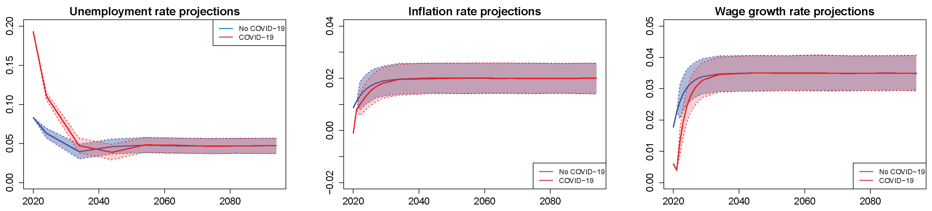
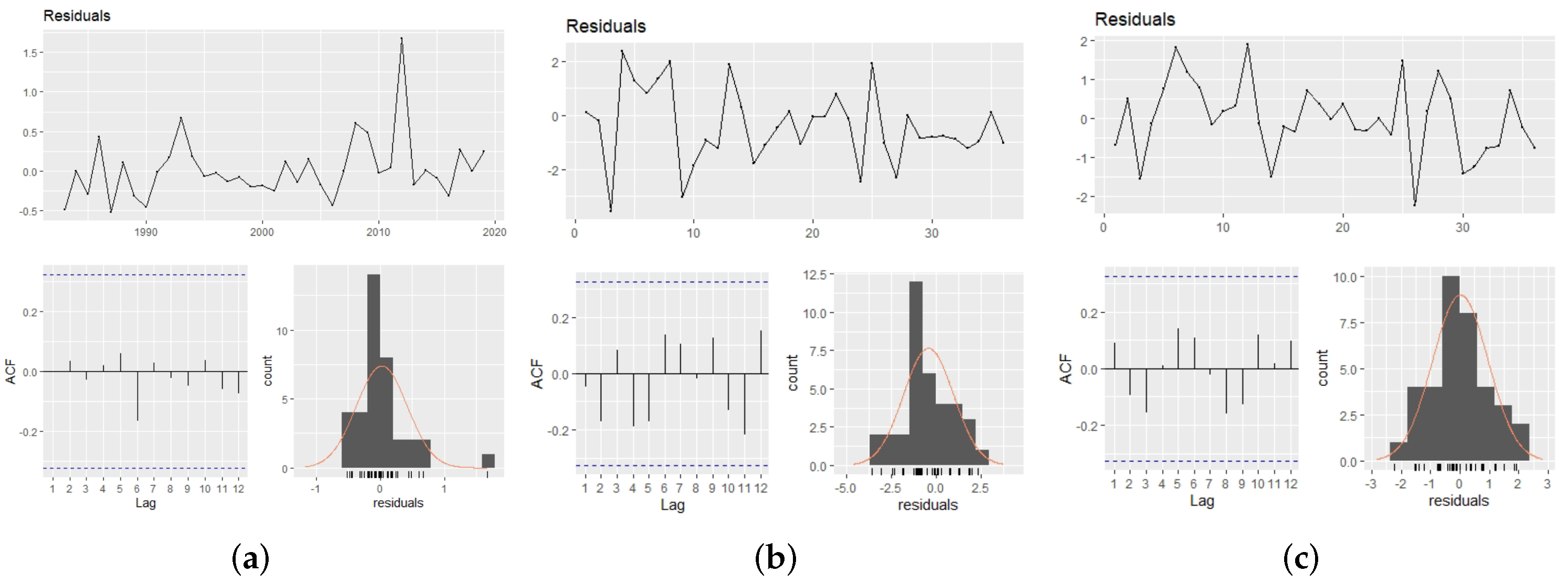
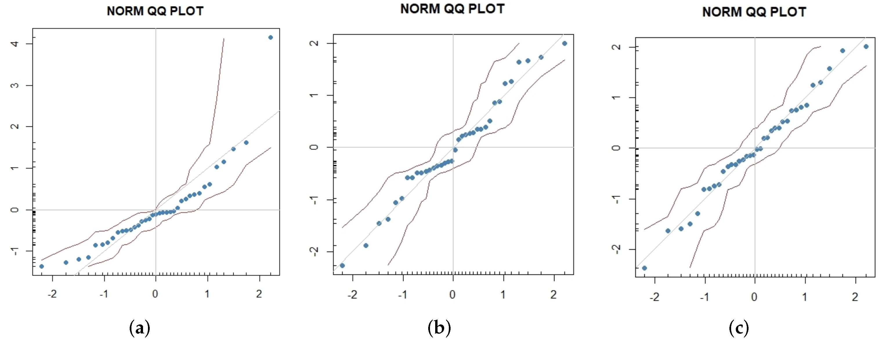
2.2. Macroeconomic Variables Modeling

To investigate the evolution of an NDC scheme during the COVID-19 pandemic, we have to make assumptions on the evolution of the transition probabilities and the macroeconomic variables relevant to the system. It is extremely complex to forecast the evolution of the main economic variables following the pandemic crisis. COVID-19 has led to high economic uncertainty, and projections are consequently variable, requiring particularly strong assumptions [23,24]. In particular, Ref. [24] highlight that some lessons can be learned from the global financial crisis (GFC) that occurred in 2008 in projecting the GDP values during the COVID-19 crisis and recovery period. They suggest adjusting the original GDP forecasts by an amount similar to the forecast errors made during the GFC. Other scholars have compared the impacts of the COVID-19 pandemic on the economy to those of GFC. For instance, Ref. [25] studied the efficiency of the US market for each industrial sector, during the GFC and COVID-19 pandemic. During the first, real estate, which caused the crisis, and information technology (IT) were the lowest-efficiency sectors; during the second, the materials sector, which suffered a big reduction in consumption and production, was the lowest-efficiency sector. Ref. [26] found that the COVID-19 pandemic affected the US economic activity more severely than GFC, while the opposite occurred in the recession probabilities.

However, the aim of the paper is not to provide an exact projection of the evolution of economic variables, which would be hard to reach but to measure the NDC pension system’s resilience to an economic shock produced by the COVID-19 pandemic. Therefore, in the following, we adopt some simplifying assumptions. We assume that all the transition probabilities are deterministic, except for the pensioners’ death probabilities, $p^{23}(x,t)$, which is modeled through a standard stochastic mortality model. While we model the inflation rate $i\left(t\right)$, the wage growth rate $\xi \left(t\right)$, and the unemployment rate $\upsilon \left(t\right)$ as stochastic processes, then we introduce two sources of uncertainty in the model: the demographic and the economic risk.

The data considered in the analysis refer to the time period immediately preceding the COVID-19 crisis, while the information, available at the time of writing, about the impact of the pandemic on mortality and the economy is used to determine the magnitude of the shock in the first two years of the pension system projections. Finally, we suppose that the demographic variables are independent from the economic variables. Details on the model selection process are provided in the following.

When dealing with the macroeconomic variables modeling, autoregressive (AR), autoregressive integrated moving average (ARIMA), and vector autoregressive (VAR) models and their variants are, by far, the most popular time series models in the macroeconomic literature. We can mention several contributions relating to modeling and forecasting the macroeconomic variables considered in this paper. For instance, ref. [27] analyzed the forecasting performance of ARIMA models, bivariate vector autoregressive moving average (VARMA) models, threshold autoregressive (TAR) models, and Markov switching autoregressive (MSA) models applied to the US unemployment rate. Ref. [28] modeled the real wage growth rate implied in the forecasts of the Social Security trust fund as an AR(1) constrained to a fixed value in the long run. Ref. [29] developed forecasts for some macroeconomic variables (inflation and unemployment rate included) in the Euro area using AR and VAR models. Ref. [30] considered both univariate and multivariate linear time series models (random walk, AR, VAR) for forecasting Euro area inflation. Ref. [31] used VAR models for obtaining forecasts for Swiss inflation, while [32] analyzed the performance of VAR and ARIMA models (in addition to factor models) for forecasting Austrian inflation. Ref. [33] used AR and VAR models to forecast a set of US macroeconomic time series. Ref. [34] provided predictions for macroeconomic variables like the unemployment rate using VAR models and considering data revisions. Ref. [35] used a time-varying coefficients VAR with stochastic volatility to predict the inflation rate and unemployment rate in the US. Ref. [36] used ARIMA and VAR models to forecast the Italian youth unemployment rate combining official and Google Trends data.

However, in recent years, advanced non-linear time series methods and artificial neural networks or hybrid approaches combining linear models with autoregressive neural networks have become popular also in the macroeconomic literature. Ref. [37] studied the forecast accuracy of AR, smooth transition autoregressive, and autoregressive neural network (AR-NN) time series models for a wide set of macroeconomic variables of the G7 economies. Refs. [38,39] forecast the unemployment rate, respectively, for some European countries and some Asian countries, using ARIMA models combined with AR-NN and support vector machines. Ref. [40] forecast inflation of the Euro using Jordan and feedforward neural networks.

Following the relevant literature, we model the inflation rate and wage growth rate through VAR models. The unemployment rate is modeled apart using an ARIMA process as it has a different nature from inflation and wage growth rate. These latter variables represent rates of change between two consecutive years, while the unemployment rate is a ratio between specific groups of people. Each macroeconomic variable is projected using a mean-reversion to an exogenous long-run trend, similar to the approach in [41] (the authors observed that the structural changes that happened in recent years in some key variables of a social security system, such as fertility, productivity, and interest rate, resulted in mean values that differ from the average of their past values. After much experimentation, they found that satisfactory forecasts were obtained by pre-specifying the long-term means of the series rather than estimating them from the data), where the main reason to include an exogenous long-run trend is to control the long-run simulations to obtain realistic forecasts. This approach meets our scope, which is to obtain reliable forecasts in line with the expected long-term trends and give a robust stochastic structure to our framework to study the impact of COVID-19 on the NDC pension systems. Our approach is also compliant with the literature dealing with the financial sustainability of the pension systems, which generally adopts the hypothesis that the macroeconomic variables are deterministic and consistent with the paths projected by the main financial institutions [22,42,43] or makes a trivial hypothesis [44].

For our analysis, we consider the following data provided by the Italian National Institute of Statistics (ISTAT):

• The unemployment rate of the male population aged 25–75 in the years 1983–2015; the rates for the residual period (2016–2019) are estimated by regression using the unemployment rate of the male population aged 15–64. These data provide values of $\upsilon \left(t\right)$.
• The wage growth rate in the years 1983–2015, and the gross contractual hourly remuneration of employees for the last four years, which are used to estimate $\xi \left(t\right)$.
• The consumer price index for blue and white-collar worker households (FOI) in the years 1983–2019, which are used to estimate $i\left(t\right)$.

Before choosing the model, for all the macroeconomic variables, we initially inspect their stationarity using the Phillips–Perron (PP) test (null hypothesis: no stationarity) and the Kwiatkowski–Phillips–Schmidt–Shin (KPSS) test (null hypothesis: stationarity), both at a 5% significance level. The results show that the wage growth rate and inflation rate are stationary, leading to reject the vector error correction model (VECM), which adds to the VAR model an error-correction term, modeling a linear combination of the variables. Then, we analyze the structure of the causal relationships between these variables through the Granger causality test, which is a statistical test for determining whether a one-time series is useful for forecasting another. We perform the Granger causality test at a 10% level. Then, we look for the optimal number of parameters in the VAR model using the R package autoarima and test the validity of the model through a set of well-known goodness of fit measures: the Akaike Information Criterion (AIC), the Hannan-Quinn information criterion (HQ), the Schwarz Criterion (SC) and the Final Prediction Error (FPE). We find VAR(1) as the best model. In the case of unemployment rate, we cannot reject the null hypothesis of PP and KPSS tests, thus questioning the presence of stationarity. Consequently, we consider the ARMA models and not the ARIMA.

The choice of the best model for each macroeconomic variable is made by analyzing the plots of the Auto-Correlation function (ACF) and Partial Auto-Correlation functions (PACF), the Akaike Information Criterium (AIC), and checking the stationarity of residuals and their normality distributions (see Appendix A.1). As a result, we model the inflation rate and wage growth rate through a VAR(1) with an exogenous long-run trend of 3.5% for the wage growth rate and 2% for the inflation rate, and the unemployment rate through an AR(4) with a 4.7% exogenous long-run trend in line with the long-term values adopted by the Ministry of Finance for the long-term projections of the national pensions expenditure [45]. Therefore, the unemployment rate considering the exogenous long-run trend ${\tau }_{\upsilon }$, and denoted as $\overline{\upsilon }\left(t\right)=\upsilon \left(t\right)-{\tau }_{\upsilon }$, is described as follows:

$$\overline{\upsilon }\left(t\right)=c_{\overline{\upsilon }}+\sum _{i=1}^4{\phi }_i·\overline{\upsilon }(t-i)+e_{\overline{\upsilon }}\left(t\right)$$

(8)

where ${\phi }_1,\dots ,{\phi }_4$ are the parameters of the model, $c_{\overline{\upsilon }}$ is a constant serving as the intercept of the model, and $e_{\overline{\upsilon }}\left(t\right)$ is a white noise process. While the inflation rate and the wage growth rate considering the exogenous long-run trends ${\tau }_i$ and ${\tau }_{\xi }$, which are denoted as $\overline{i}\left(t\right)=i\left(t\right)-{\tau }_i$ and $\overline{\xi }\left(t\right)=\xi \left(t\right)-{\tau }_{\xi }$, respectively, are jointly modeled as a VAR(1) process:

$$\overline{i}\left(t\right)=c_{\overline{i}}+{\varphi }_1·\overline{i}(t-1)+{\varphi }_2·\overline{\xi }(t-1)+e_{\overline{i}}\left(t\right)$$

(9)

$$\overline{\xi }\left(t\right)=c_{\overline{\xi }}+{\theta }_1·\overline{i}(t-1)+{\theta }_2·\overline{\xi }(t-1)+e_{\overline{\xi }}\left(t\right)$$

(10)

where ${\varphi }_1$, ${\varphi }_2$, ${\theta }_1$ and ${\theta }_2$ are the parameters of the model, $c_{\overline{i}}$ and $c_{\overline{\xi }}$ are constants serving as the intercept of the model, and $e_{\overline{i}}\left(t\right)$ and $e_{\overline{\xi }}\left(t\right)$ are zero-mean white noise processes. Equation (9) implies that the inflation rate in a certain year is related not only to the previous inflation rate (through parameter ${\varphi }_1$) but also to the previous wage growth rate (through parameter ${\varphi }_2$). A similar consideration can be made for the wage growth rate in Equation (10).

2.3. Mortality Modeling

The mortality data contain 35 historical observations in the years 1983–2017 given from the Human Mortality Database. For the years 2018–2019, we use values estimated by the Lee–Carter model. For the pensioners’ probability of death, we assume that the number of deaths $D(x,t)$ follows a Poisson distribution: $D(x,t)\sim Poisson\left(E\right(x,t\left)m\right(x,t\left)\right)$, where $E(x,t)$ are the exposure to risk, and $m(x,t)$ are the central death rate for age x and year t. For mortality modeling, we refer to the Lee–Carter model [46], which is the most widely used mortality model in the literature. The Lee–Carter model describes the logarithm of the central death rates by age x and time t as:

$$logm(x,t)={\alpha }_x+{\beta }_x{\kappa }_t$$

(11)

where ${\alpha }_x$ is the age-specific parameter describing the average age profile of mortality, ${\kappa }_t$ is the level of mortality at time t, and ${\beta }_x$ is the age pattern of mortality change at age x. From the previous equation, we can easily obtain the death probabilities $p(x,t)$ using the following formula:

$$p(x,t)=1-exp(-m(x,t\left)\right)$$

(12)

We develop the mortality projections by forecasting ${\kappa }_t$ through an Auto-Regressive Integrated Moving Average (ARIMA) process. Following the standard literature, we model ${\kappa }_t$ as an ARIMA(0,1,0):

$${\kappa }_t={\kappa }_{t-1}+\delta +ϵ\left(t\right)$$

(13)

where $\delta$ is the drift parameter and $ϵ\left(t\right)$ are the error terms, which are normally distributed with null mean and variance ${\sigma }_k^2$, $ϵ\left(t\right)\sim N(0,{\sigma }_{\kappa }^2)$. The plots of the estimated parameters are reported in Appendix A.2.

2.4. The COVID-19 Macroeconomic and Demographic Scenario

We denote $j\left(t\right)=\left\{j_{\upsilon }\left(t\right),j_i\left(t\right),j_{\xi }\left(t\right)\right\}$ as the COVID-19 shock over the macroeconomic variables here considered, where $j_{\upsilon }\left(t\right)$ represents the shock on the unemployment rate, $j_i\left(t\right)$ represents the shock on the inflation rate, and $j_{\xi }\left(t\right)$ represents the shock on the wage growth rate. We set $j\left(t\right)=0$ for all t with the exception of $t^{*}$ and $t^{*}+1$, where $t^{*}=2020$. Therefore, $\overline{\upsilon }\left(t\right)$, $\overline{i}\left(t\right)$ and $\overline{\xi }\left(t\right)$ under the COVID-19 scenario are, respectively, modeled as follows:

$$\overline{\upsilon }\left(t\right)=c_{\overline{\upsilon }}+\sum _{i=1}^4{\phi }_i·\overline{\upsilon }(t-i)+e_{\overline{\upsilon }}\left(t\right)+j_{\upsilon }\left(t\right)$$

(14)

$$\overline{i}\left(t\right)=c_{\overline{i}}+{\varphi }_1·\overline{i}(t-1)+{\varphi }_2·\overline{\xi }(t-1)+e_{\overline{i}}\left(t\right)+j_i\left(t\right)$$

(15)

$$\overline{\xi }\left(t\right)=c_{\overline{\xi }}+{\theta }_1·\overline{i}(t-1)+{\theta }_2·\overline{\xi }(t-1)+e_{\overline{\xi }}\left(t\right)+j_{\xi }\left(t\right)$$

(16)

Concerning the COVID-19 impact on mortality, many proposals have been made in the literature to model adverse mortality jumps. Ref. [46] suggest to introduce a dummy variable in the time index process to treat the impact of Spanish flu on US mortality. According to this approach, denoting $j_{\kappa }\left(t\right)$ as the COVID-19 mortality shock, ${\kappa }_t$ should be modeled as:

$${\kappa }_t={\kappa }_{t-1}+\delta +ϵ\left(t\right)+j_{\kappa }\left(t\right)$$

(17)

Since then, many models that incorporate adverse jumps in mortality have been proposed in the literature, most of them with the aim to value catastrophic mortality bonds. For instance, Ref. [47] considered a compound Poisson process to model permanent mortality jumps. Ref. [48] used independent Bernoulli distribution for transitory jump occurrence and normal distribution for jump severity. Ref. [49] proposed a stochastic diffusion model with double-exponential jumps. Recently, Ref. [50] used a Lee–Carter model with a jump diffusion process and a lognormal renewal process for modeling the arrival of mortality jumps.

Most of the proposed models assumed that the sensitivity of each age to the mortality jumps was the same as that of general mortality improvements, which is not supported by the empirical evidence. To avoid this limitation, Ref. [51] explicitly introduced an age pattern of temporary adverse mortality jumps distinct from that of general mortality improvements, while [52] proposed two alternative models: in the first, the age pattern of jump effects is represented through a separate constant vector; in the second, they assumed that jump effects for different age groups are not perfectly correlated, allowing the age response to different mortality jumps to be different.

Since in our paper, the objective is not to model the effect of future adverse jumps on mortality but to estimate only the impact of the COVID-19, we propose a simple solution consisting of adding an extra term for the year 2020, ${\alpha }_{x,2000}$, to the log mortality rates, which allows representing the shift of mortality age profile due to the pandemic:

$$logm(x,t)={\alpha }_x+{\alpha }_{x,2000}+{\beta }_x{\kappa }_t$$

(18)

The increase in mortality due to COVID-19 has affected both the working and retired populations. A comparison of deaths by age group in 2020 and 2019 (see [53]) shows that only 6.4% of extra deaths in 2020 referred to the 15–64 age group. On the Italian population as a whole, the highest number of deaths recorded in the 15–64 age group in 2020 compared to 2019 is just over 7000. Thus, the effect of extra mortality due to COVID-19 on the total working population is negligible as well as its impact on employment equilibrium. Hence, we can conclude that the number of employees has much more been influenced by the change in the unemployment rate rather than by the change in mortality rates. For this reason, we have neglected the effect of COVID-19 mortality on the working population and measured only the effect on the retired population.

3. Numerical Application

3.1. Main Assumptions

We consider a reference population built from the demographic and economic structure of the National Employees’ Pension Fund members (FPLD) in 2019, taken from the Italian National Institute of Social Security (data available at www.inps.it). Specifically:

• The initial age distribution of both actives and pensioners, the initial wage distribution by age, and the initial pension benefits distribution by age derive from the corresponding observed distribution of the FPLD pension scheme.
• The new actives’ age distribution $d_z^1(x,t)$ comes from the observed age distribution of actives with a past service duration of less than 2 years in 2019.
• Analogously for the new unemployed population’s age distribution, $d_z^4(x,t)$, which we supposed to be equal to the new actives’ age distribution.
• $d_z^1(x,t)$ and $d_z^4(x,t)$ are assumed constant over time.
• $N^1\left(0\right)$, which is the initial active population, includes 1000 males.
• The initial number of pensioners is fixed by the dependency ratio of the FPLD pension scheme, i.e., $N^2\left(0\right)=N^1\left(0\right)·D\left(0\right)$ with $D\left(0\right)=43.4\%$.

With regard to the transition probabilities, we made the following assumptions:

• We assume that all the actives retire at age 63; therefore, $p^{12}(x,t)=0$$\forall x<63$ and $p^{12}(x,t)=1$$\forall x\ge 63$. Age 63 has been chosen consistently with the average retirement age of Italian employees in 2019.
• We assume that all the unemployed retire at age 63 ($p^{42}(x,t)=0$$\forall x<63$ and $p^{42}(x,t)=1$$\forall x\ge 63$).
• We set aside the mortality of the active population due to the characteristics of the Italian NDC scheme that does not consider the distribution of inheritance gains from people who die before the earliest possible retirement age. Hence, $p^{13}(x,t)=0$ for all ages and time.
• We make the same assumption for the unemployed, $p^{43}(x,t)=0$$\forall x,t$.
• The death probabilities of pensioners, $p^{43}(x,t)$, are assumed equal to the probabilities for the general Italian population.
• The term ${\alpha }_{x,2000}$ in Equation (18) is estimated from the difference between the observed and expected death rates in 2020.

With regard to the economic variables, we made the following assumption:

• Coherently with the macroeconomic assumptions of the Ministry of Finance for the long-term projection of the national pension expenditure [45], we suppose that the GDP growth rate equals the sum of the active population’s growth rate, growth rate of labor productivity and inflation rate.
• Following the prevailing literature (see for example [19,42,54,55,56]), we suppose that the individual wage’s growth rate equals the labour productivity’s growth rate.
• Following the structure of the Italian pension scheme, the notional rate $g\left(t\right)$ is set equal to the GDP growth rate, and the pension indexation rate $\lambda \left(t\right)$ equals the inflation rate $i\left(t\right)$.
• As specified in Section 3, to deal with the influence of COVID-19 on the Italian system, we include a shock in $t^{*}=2020$ and $t^{*}+1$ on the inflation rate $i\left(t\right)$, the wage growth rate $\xi \left(t\right)$, and the unemployment rate $\upsilon \left(t\right)$.

  -

  The shock level for the inflation rate is based on the estimates provided by the European Economic Forecast in 2021 [57].

  -

  The shock for the wage growth rate is estimated by [58]

  -

  The shock for the unemployment rate is estimated from [59].

The contribution rate $c\left(t\right)$ is set to 30% according to the Italian pension system (the Italian NDC legislation fixes the contribution rate at 33%. At retirement, the pension benefit is calculated by dividing the notional amount by the sum of the annuity rate for the pensioner and of the annuity rate for the pensioner’s survivors. Both annuity rates are determined as an average between male and female rates. The weight of the annuity rate for the pensioner on the sum is close to 91%. In our application, we disregard survivors’ benefits. Therefore, to obtain benefits values consistent with the benefits provided in the Italian system, we reduce the contribution rate to 30% (≃$33\%·91\%$)).

We develop the analysis for 75 years, which is the period typically used in actuarial reports evaluating the financial sustainability of pension systems (see, for example, the United States and Canada). A 75-year period is necessary if we want to study the baby-boom cohort until its elimination from the pension system, thus almost deleting its influence on the final demographic structure of the system. The last long-term projections of Italian pension expenditure produced by the Ministry of Finance in 2020–2070 [45] use 50 years. The numerical analysis has three phases. We first select the model and its parameters for the macroeconomic variables and the parameters of the Lee–Carter model describing the mortality of retirees. Secondly, we develop the stochastic projections of the NDC key variables with and without the COVID-19 pandemic by simulating 10,000 paths. Finally, we analyze the effect of the COVID-19 crisis in the hypothesis of its different impacts on the unemployment rate.

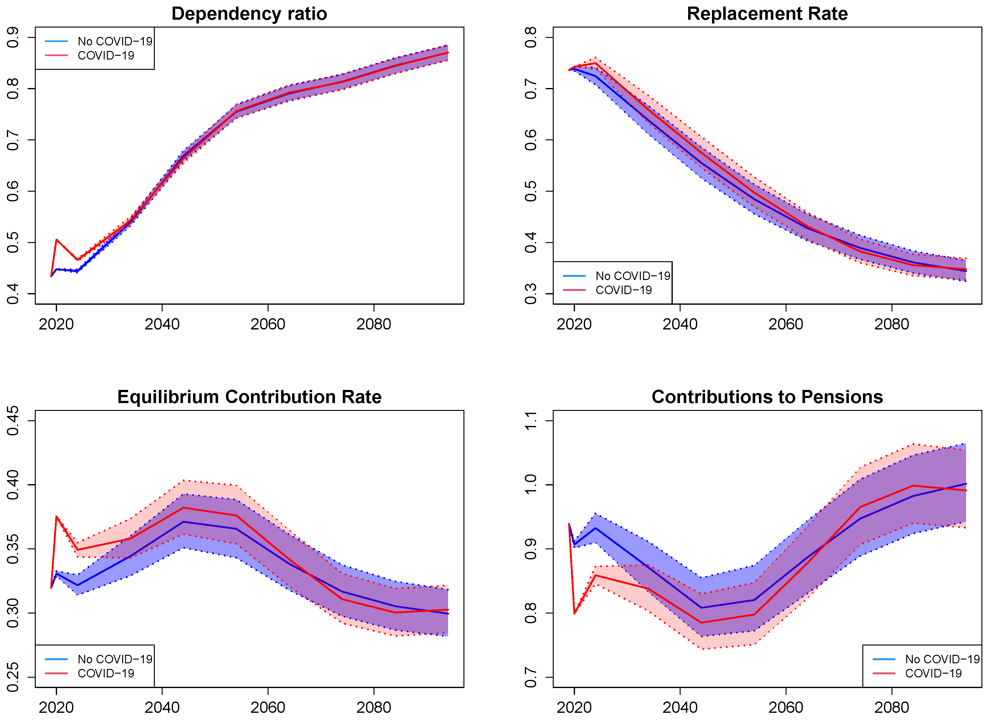
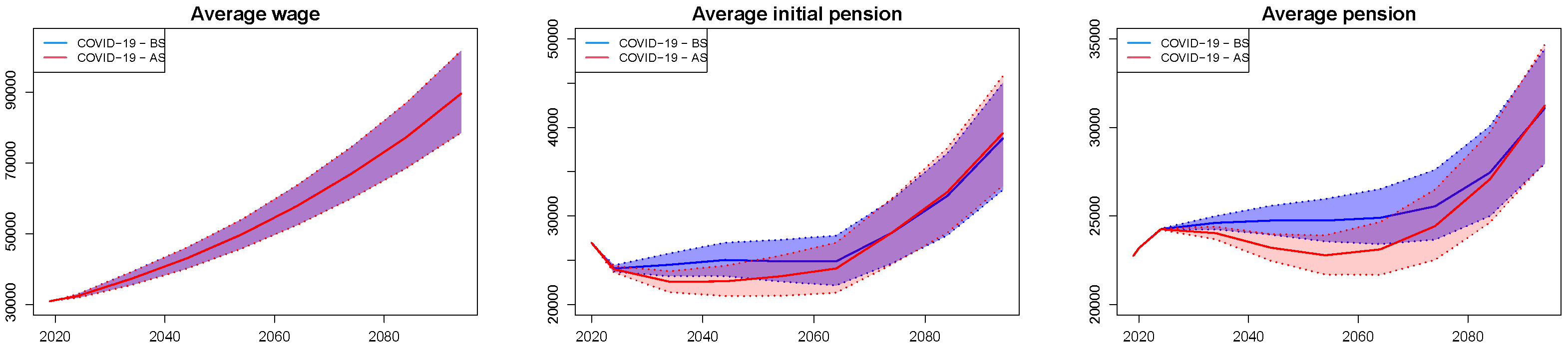
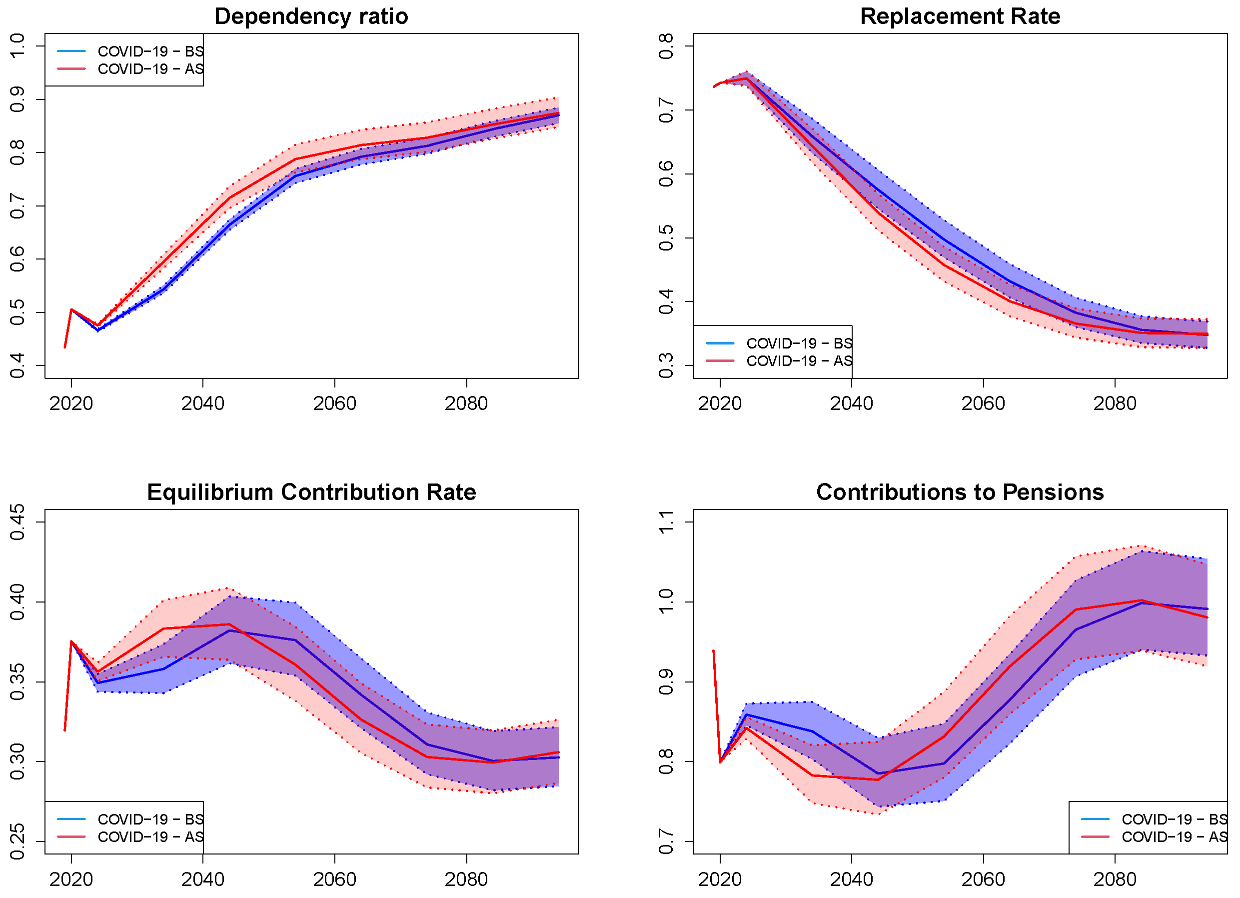
3.2. Baseline Results with and without COVID-19

Figure 1 shows the projected values over the years 2019–2094 for unemployment rate, inflation rate and wage growth rate, while Figure 2 illustrates the evolution of average wage, average initial pension and average pension (all net of inflation). The No COVID-19 scenario is depicted in blue, while the COVID-19 scenario is depicted in red.

From Figure 1, we can appreciate the strong impact of the COVID-19 shock on the unemployment rate. The rates in the two scenarios are very different in the first 15 years of the projection, and the differences appear negligible only from 2055. The initial shock on the inflation rate and wage growth rate is about −1%. However, while inflation rises immediately, the wage growth rate is assumed to shock further in the second year. As a result, inflation is approaching its long-term rate faster than wage growth. Differences in the wage growth rate between the No COVID-19 scenario and the COVID-19 one will become negligible only from 2030. This induces a reduction in the average wage net of inflation (before the payment of contributions) of 4%, ten years from the crisis. Since then, the inflation rate and wage growth rate will follow a similar pattern. Therefore, the COVID-19 shock impact on the average wage (net of inflation) will persist over time (Figure 2—left panel).

The biggest impact of the COVID-19 shock on the initial pension (net of inflation) is after 2040 (Figure 2—central panel). Since then, the nominal account of the new pensioners will have suffered for a large number of years from the negative effects of COVID-19. The greatest reduction is obtained for cohorts that begin to work during the crisis (−8% in 2064). With reference to the average pension (net of inflations) (Figure 2—right panel), the impact of COVID-19 is more visible in the long run. The shock affects the notional account of the active population that will originate the pension benefit in the subsequent years in three ways: firstly, some workers will be deprived of their jobs for the growing unemployment rate.Secondly, the reduction of the average wage results in a reduction in the average contributions paid (at the same contribution rate). Thirdly, GDP reaches negative values, implying a reduction of the notional rate of return in 2020. The COVID-19 impact on average pensions is only −0.2% after 5 years and −0.9% after 15 years, but it is −5.7% in 2074 and is partially reduced to −3.1% at the end of the time horizon (the average pension accounts for 24,615 Euros in the COVID-19 scenario vs. 24,847 Euros in the No COVID-19 one in $t=$ 2034, 25,610 Euros vs. 27,164 Euros in $t=$ 2074, and 31,168 Euros vs. 32,162 Euros in 2094, all net of inflation).

Figure 3 illustrates the dynamics of dependency ratio, replacement rate, equilibrium contribution rate, and the ratio of contributions to pensions for the baseline scenario (in blue color) and for the COVID-19 scenario (in red color). The expected values of the dependency ratio, replacement rate, and equilibrium contribution rate over the 75-year time horizon under the No COVID-19 scenario and the COVID-19 scenario are both reported in

Table 1. Evolution of the expected values of Dependency Ratio (DR), Replacement Rate (RR), Equilibrium Contribution Rate (ECR) and Contributions to Pensions (CP) under the No-COVID-19 scenario (No COVID-19) and the COVID-19 scenario (COVID-19), and the percentage change between the two scenarios ($\Delta \%$ COVID-19).

Year		2019	2020	2024	2034	2044	2054	2064	2074	2084	2094
DR	No COVID-19	0.434	0.448	0.444	0.539	0.669	0.755	0.791	0.813	0.845	0.870
	COVID-19		0.506	0.466	0.543	0.664	0.756	0.792	0.813	0.844	0.870
	$\Delta \%$ COVID-19		12.9%	4.9%	0.7%	−0.7%	0.1%	0.2%	−0.1%	−0.1%	0.0%
RR	No COVID-19	0.736	0.738	0.724	0.639	0.556	0.485	0.429	0.390	0.362	0.345
	COVID-19		0.743	0.750	0.659	0.576	0.498	0.432	0.383	0.356	0.348
	$\Delta \%$ COVID-19		0.5%	3.5%	3.2%	3.6%	2.7%	0.8%	−1.8%	−1.6%	1.0%
ECR	No COVID-19	0.320	0.331	0.322	0.345	0.372	0.366	0.339	0.317	0.305	0.300
	COVID-19		0.375	0.349	0.358	0.382	0.376	0.342	0.311	0.301	0.303
	$\Delta \%$ COVID-19		13.5%	8.6%	3.9%	2.9%	2.9%	1.0%	−1.9%	−1.6%	1.1%
CP	No COVID-19	0.939	0.907	0.933	0.872	0.809	0.822	0.887	0.948	0.984	1.003
	COVID-19		0.799	0.859	0.839	0.786	0.799	0.878	0.966	1.001	0.993
	$\Delta \%$ COVID-19		−11.9%	−7.9%	−3.8%	−2.9%	−2.8%	−1.0%	2.0%	1.6%	−1.0%

, together with the percentage change between the two scenarios. Expectation and quantile at a 0.5% level of the final reserve fund ($E\left[F\right(T\left)\right]$ and $Q_{0.5\%}\left[F\left(T\right)\right]$, respectively) and their absolute change are reported in

Table 2. Expectation ($E\left[F\right(T\left)\right]$) and quantile at 0.5% ($Q_{0.5\%}\left[F\left(T\right)\right]$) of the final reserve fund under the No COVID-19 scenario (No COVID-19) and the COVID-19 scenario (COVID-19), and the absolute change between the two scenarios ($\Delta$ COVID-19).

Scenario	$\mathit{E}\left[\mathit{F}\right(\mathit{T}\left)\right]$	${\mathit{Q}}_{0.5\%}\left[\mathit{F}\left(\mathit{T}\right)\right]$
No COVID-19	−1,028,956,271	−1,529,673,097
COVID-19	−1,160,895,524	−1,620,110,175
$\Delta$ COVID-19	−131,939,253	−90,437,078

for both scenarios.

From Table 1, we observe that the dependency ratio increases in 75 years from 0.434 to 0.870 in the two scenarios, highlighting a minimal influence of COVID-19 in the medium/long run (with a percentage variation between the two scenarios of less than 1% from 2034 onwards). In both scenarios, however, the number of pensioners per active redoubles in the observed period for the increment in life expectancy, consequently worsening the financial sustainability of the system. In the short term, we notice a still relevant effect of COVID-19 on the dependency ratio following the unforeseen increase in the unemployment rate: in 2020, the pandemic shock caused, on average, a 0.058 rise of the dependency ratio (0.506 vs. 0.448, with a percentage change of +12.9%). The increase falls to 0.022 after 5 years and becomes 0.007 after 15 years. The dependency ratio is influenced by the mortality shock, which lowers the number of pensioners, and by the unemployment shock, which decreases the number of workers. However, the latter shock is characterized by a small variability in the forecast horizon (for example, in $T=2094$, the standard deviation is approximately 0.0113 for both scenarios, while the 90% confidence interval of $D\left(t\right)$ is (0.851, 0.889) for both scenarios).

The replacement rate declines by 0.736 to 0.345 in the No COVID-19 scenario and 0.348 in the COVID-19 one (Table 1). These findings pose the question of the social adequacy of the Italian pension system in the medium/long run independently from the shock occurrence. Actually, in the early years, the COVID scenario presents better social adequacy than the No COVID scenario. After 5 years, the replacement rate in the COVID scenario is 0.026 higher (3.5% increase) than in the No COVID one. The reason is due to the pandemic shock that has an immediate impact on the average wage and not on the average pension. In subsequent years, the average pension is also affected by the pandemic. As a result, the replacement rate decreases more rapidly in the COVID-19 scenario and becomes about −1.8% compared with the No COVID scenario in 2074. At the end of the time horizon, this difference is reduced to 1%. The model adopted for the evolution of the wage implies that the wage growth rate, $\xi \left(t\right)$, moves toward a long-term value of ${\tau }_{\xi }$. This involves that in the long run, the COVID-19 and No COVID-19 scenarios have close growth rates, but monetary values in the first scenario remain lower as a result of the shock. Lower wages in the COVID-19 scenario, even in the long run, lead to minor contributions and consequently lower notional amounts and then lower pensions. This long-term effect on the monetary values of wages and pensions does not affect the replacement rate, which is a relative measure.

In the No COVID-19 scenario, the equilibrium contribution rate (it is the ratio between total pensions and total wages. It could be rewritten as the product of dependency ratio and replacement rate) fluctuates from a minimum of 0.3 (at the end of the projection horizon) to a maximum of 0.372 (in 2044) (Table 1). In fact, the replacement rate and the dependency ratio shift in opposite directions. The effect of the dependency ratio increase prevails until 2044, while the effect of the replacement rate reduction predominates later. This latter ratio shows sustainable values over time and, finally, is very close to the contribution rate. The COVID-19 shock has an immediate adverse impact on the system by increasing the equilibrium contribution rate (0.375 in 2020 and 0.349 in 2024, with an increase compared to the No COVID-19 scenario equal to 13.5% and 8.6%, respectively), which reduces in the following years (less than 2% from 2064 onwards).

Looking at the liquidity of the system, we consider the ratio between contributions income and pensions expenditure, $\frac{C\left(t\right)}{P\left(t\right)}$. If $\frac{C\left(t\right)}{P\left(t\right)}=1$, the PAYG pension system is in equilibrium. If $\frac{C\left(t\right)}{P\left(t\right)}>$1, the reserve fund $F\left(t\right)$ is increased. The opposite is true when $\frac{C\left(t\right)}{P\left(t\right)}<1$. We find that the average ratio remains in the range of (0.809, 1.003) during the whole time horizon in the No COVID-19 scenario and in the range of (0.786, 1.001) in the COVID-19 one (Table 1). It already shows significant variability in the medium/long term, i.e., its standard deviation in both scenarios is close to 0.03 for $t=2034$ and the 90% confidence interval, at the end of the time horizon, is (0.924, 1.084) in the No COVID-19 scenario and (0.916, 1.073) in the COVID-19 one. The pandemic shock remarkably reduces $\frac{C\left(t\right)}{P\left(t\right)}$ in 2020 (−11.9%), which partially recovers in the medium term (−3.8% in 2034) and backs to the pre-pandemic value in the long term (−1% in 2094).

The overall pandemic effect (joint with the timing of the deficits/surpluses) can be analyzed by the reserve fund in the final year, $F\left(T\right)$ (Table 2). Without the shock, the pension system is not financially sustainable, providing an expected final fund $E\left[F\right(T\left)\right]$ of about −1.029 million euros. To better understand the size of the deficit, it must be considered that the amount of total wages in the same year amounts to 1.653 million euros. Therefore, the liability is equal to 62% of the total wages. In the COVID-19 scenario, $E\left[F\right(T\left)\right]$ is about −1.161 million euro, while total wages in the same year account for 1.488 million euro (the liability is equal to 78% of the total wages). Therefore, the shock has worsened the financial sustainability of the system.

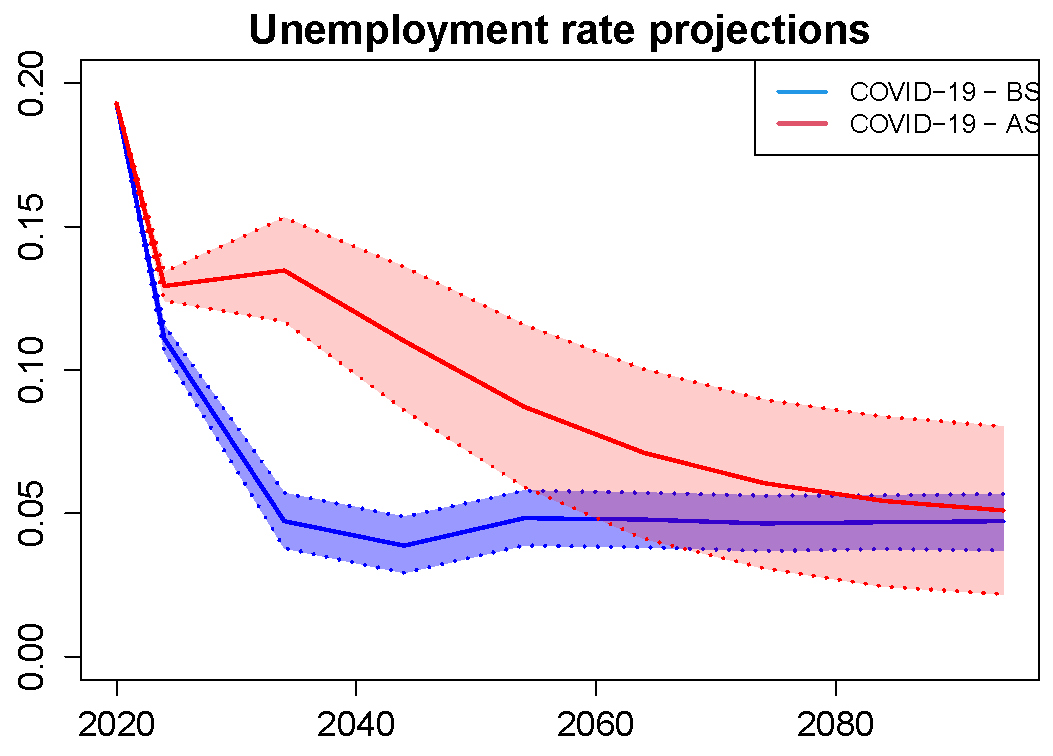
3.3. Unemployment Rate Sensitivity Analysis

To evaluate how the results vary with some of the key parameters, we develop a sensitivity analysis. In particular, in light of the findings discussed in Section 3.2, it is clear that the unemployment rate is the key economic variable. This result is consistent with the theoretical analysis that demonstrates the relevance of the unemployment rate on the balance of the pension system and how its unexpected fluctuations can generate deficits (or surpluses) (see [60]).

First, the unemployment rate influences the evolution of the dependency ratio. Secondly, it influences the evolution of GDP, which is the rate of return of the notional amount, and thus the amount of future pensions. In particular, our goal is to measure how the results change if it takes longer for workers unemployed due to the pandemic to find a new job. We define a new scenario increasing the AR term in Equation (8) by 5% (COVID-19—AS), leading the unemployment rate process to more slowly converge toward the long-run trend. Therefore, we are assuming a worsening of the labor market dynamics. We compare the results of the COVID-19—AS scenario to the scenario with the standard evolution of the unemployment rate (COVID-19—BS).

The effect of varying the process parameters followed by the unemployment rate (Figure 4) on the results is shown in Figure 5 and Figure 6, and

Table 3. Evolution of the expected values of Dependency Ratio (DR), Replacement Rate (RR), Equilibrium Contribution Rate (ECR) and Contributions to Pensions (CP) under the COVID-19 scenario with standard evolution of the unemployment rate (COVID-19—BS) and the COVID-19 scenario with alternative evolution of the unemployment rate (COVID-19—AS), and the percentage change between the two scenarios ($\Delta \%$ AS).

Year		2019	2020	2024	2034	2044	2054	2064	2074	2084	2094
DR	COVID-19—BS	0.434	0.506	0.466	0.543	0.664	0.756	0.792	0.813	0.844	0.870
	COVID-19—AS		0.506	0.475	0.595	0.715	0.788	0.815	0.829	0.854	0.875
	$\Delta \%$ AS		0.0%	2.0%	9.6%	7.7%	4.3%	2.8%	2.0%	1.1%	0.6%
RR	COVID-19—BS	0.736	0.743	0.750	0.659	0.576	0.498	0.432	0.383	0.356	0.348
	COVID-19—AS		0.743	0.750	0.644	0.540	0.458	0.401	0.366	0.351	0.350
	$\Delta \%$ AS		0.0%	0.0%	−2.3%	−6.2%	−8.0%	−7.1%	−4.4%	−1.4%	0.5%
ECR	COVID-19—BS	0.320	0.375	0.349	0.358	0.382	0.376	0.342	0.311	0.301	0.303
	COVID-19—AS		0.375	0.356	0.383	0.386	0.361	0.327	0.303	0.300	0.306
	$\Delta \%$ AS		0.0%	2.0%	7.1%	1.0%	−4.1%	−4.5%	−2.5%	−0.3%	1.1%
CP	COVID-19—BS	0.939	0.799	0.859	0.839	0.786	0.799	0.878	0.966	1.001	0.993
	COVID-19—AS		0.799	0.842	0.783	0.778	0.833	0.920	0.992	1.004	0.982
	$\Delta \%$ AS		0.0%	−2.0%	−6.6%	−1.0%	4.3%	4.8%	2.6%	0.3%	−1.0%

.

In the alternative scenario, the initial average pension is reduced even further before 2040 due to the persistence of high unemployment rates. On the contrary, in the COVID baseline scenario, the employment growth in the first 15 years allows for offsetting the initial shock and the lower values of contributions. As a result, the average pensions in COVID-19—AS are lower than in COVID-19—BS up to 2085. In the COVID-19—AS scenario, the dependency ratio grows faster (0.595 versus 0.543 in 2034, an increase of 9.6%), but the long-term values are roughly aligned. In the period 2040–2070, the average pension in the COVID-19—AS scenario is substantially lower than in the COVID-19—BS scenario as a consequence of the reduced contributions due to unemployment and the slower recovery of the GDP (note that as previously specified, we have assumed that the GDP is given by the sum of the labor productivity’s growth rate, the active population’s growth rate, and the inflation rate). Therefore, in the medium term, the replacement rate in the COVID-19—AS scenario is lower than in the COVID-19—BS one (0.458 versus 0.498 in 2054; 8% reduction), but at the end of the period, these values converge. No change in the average wage is assumed in the two scenarios. We can state that the Italian NDC system will have a social adequacy problem in the mid-term if the impact of the shock on the unemployment rate will be longer than expected. In addition, concerning ECR, the alternative scenario is more critical than the basic one. In 2034, the ECR in the COVID-19—AS is equal to 0.383 versus 0.358 in the COVID-19—BS (7.1% increase). However, the reduction in average pensions in the following years leads to a reduction of ECR in 2064 (0.327 versus 0.342, with a reduction of 4.5%). The CP results move in the opposite direction.

The overall effect of the alternative assumption on the unemployment evolution can be addressed by examining the reserve fund in the final year $F\left(T\right)$ (see

Table 4. Expectation ($E\left[F\right(T\left)\right]$) and quantile at 0.5% ($Q_{0.5\%}\left[F\left(T\right)\right]$) of the final reserve fund under the COVID-19—BS scenario and the COVID-19—AS scenario, and the absolute change between the two scenarios ($\Delta$ AS).

Scenario	$\mathit{E}\left[\mathit{F}\right(\mathit{T}\left)\right]$	${\mathit{Q}}_{0.5\%}\left[\mathit{F}\left(\mathit{T}\right)\right]$
COVID-19—BS	−1,160,895,524	−1,620,110,175
COVID-19—AS	−1,146,928,808	−1,600,542,927
$\Delta$ AS	−13,966,716	−19,567,248

). The results show a very similar value of $F\left(T\right)$ in the two scenarios. The persistence of high unemployment rates does not worsen the financial sustainability of the NDC system (which, however, is not achieved in both cases) due to the lowering of the average pension, which reduces the pension benefits social adequacy.

4. Discussion

The paper measures the potential impact of the unemployment and mortality rate shock produced by COVID-19 on the future evolution of the Italian pension system, concentrating on financial sustainability and social adequacy. In particular, we have shown the evolution of the equilibrium contribution rate (an index of financial liquidity), average pension (a measure of adequacy), replacement rate (a relative index of adequacy), and dependency rate (an index of sustainability). Finally, the system’s long-term financial sustainability is evaluated through the expected value and quantile at an 0.5% level of the final reserve fund. All these measures are determined under three different scenarios (No COVID-19 scenario, COVID-19 baseline scenario, COVID-19 alternative scenario) as described in the previous section. Despite the limitations arising from the difficulty of projecting the demographic and economic variables of a pension system over a long time horizon, the results enable us to make some reflections on the future of the system and how it will be affected by the pandemic. Below, we examine some of the main results obtained to try to answer the research questions we posed.

In the short–medium term, COVID-19 affects the dependency ratio due to the rapid growth of the unemployment rate. In addition, it increases the equilibrium contribution rate (that exceeds 37% in the medium term, pointing out that a fixed rate is insufficient to guarantee the liquidity of the system) and worsens the financial sustainability of the system (as shown by the reduction of the reserve fund at the end of the time horizon). This is in line with the finding of [16] that the COVID-19 pandemic will exacerbate the financial sustainability of the Romanian public pension system in the short term.

In terms of social adequacy, in the two COVID-19 scenarios, a reduction of the average pension in monetary value is observed. This does not necessarily cause a worsening of the pensioners’ economic conditions, as the value of average pensions relative to average wages (i.e., the replacement rate) does not decrease. Such a result might be compared with the findings of [17], according to which COVID-19 would produce a positive effect on future pensioners that would benefit from expected higher replacement rates at retirement.

In the long run, the main demographic and economic indicators of the COVID-19 baseline scenario tend to converge to the values assumed in the No COVID-19 one. On one hand, the pension system shows critical values for the dependency ratio and social adequacy. On the other hand, the equilibrium contribution rate approaches the fixed contribution rate (30%), and the Contributions to Pensions ratio stabilizes at values close to 1, ensuring the liquidity of the system. Long-term financial sustainability is not achieved as for the existence of medium-term imbalances between contributions and pensions (already present in the No COVID-19 scenario and more seriously in the COVID-19 scenario) and not for their long-term ratio.

The convergence of the results of the different scenarios over the long term is a consequence of the models representing the evolution of unemployment rate, inflation rate, and wage growth rate. Actually, these variables converge to the same values both in the COVID-19 and No COVID-19 scenarios. Although this is a possible limitation of the approach adopted (already discussed in the previous sections), some general considerations can be drawn.

The pandemic shock will impoverish pensioners, especially those generations that were at the beginning of their working life at the time of the crisis. However, the benefits reduction will not substantially aggravate the social adequacy of the Italian pension system in the medium–long term as the replacement rate hereafter guaranteed by the system is, in all scenarios, very low.

The pension system presents liquidity and solvency issues in the medium term that COVID-19 will aggravate. However, as observed in Section 2.1, the NDC system is characterized by an `automatic pilot’ that corrects notional amounts and pension benefits to balance contributions and benefits in the long run. The financial sustainability issues observed in the medium term are the effect of the retirement of the baby-boomers cohort that will partially benefit from the old pension calculation rules (before the introduction of the NDC system). Finally, from the results of the sensitivity analysis, we can deduce that the ability of the system to rebalance strongly depends on the speed of the return to long-term values of the unemployment rate. A social adequacy question may arise if the economic recovery were to be slower than expected.

Our analysis presents a number of limitations. Our findings are closely linked to the specific features and conditions of the Italian system and cannot be generalized to other NDC pension systems. The numerical analysis is developed on a long-term horizon (75 years) in line with most actuarial reports evaluating pension long-term financial sustainability. Nevertheless, a mathematical model can hardly be effective in predicting a complex reality such as the dynamics of a public pension system over such a long period. Therefore, our results should be considered more reliable in the short and medium-term.

5. Conclusions

This paper focused on the impact of the COVID-19 pandemic on the financial sustainability and social adequacy of the pension benefits to retirees of the Italian NDC pension system. Indeed, the restrictive measures on economic activity introduced to counter the spread of the virus are affecting the labor market by reducing employment and wages, thus probably lowering contributions income. Furthermore, the pandemic will also affect the rate of return on notional accounts, which in Italy is an average of the GDP growth rate, and future pensions will accordingly lower. Finally, the pandemic is producing an increase in mortality rates, mostly at older ages, reducing the cost of the benefits paid to pensioners.

To address the effects of COVID-19 on the Italian pension system, the macroeconomic variables involved in calculating contributions and pensions (unemployment rate, wage growth rate, and inflation rate) and mortality rates are modeled as stochastic time series. To this aim, we introduce a deterministic shock on the macroeconomic variables, whose level is based on the forecasts of the European Commission, and another one on the mortality of pensioners, whose level is based on the observed number of COVID-19 deaths registered at the time of writing.

The outcomes show that COVID-19 influences the dependency ratio only in the short run due to the rapid growth of the unemployment rate. Another consequence is the increase of the equilibrium contribution rate in the short–medium term that, however, strongly reduces in the long run. Overall, we note that the pandemic shock worsens the financial sustainability of the system as also detected by the reserve fund at the end of the time horizon. Conversely, the social adequacy of the pension system is not particularly weakened by the pandemic. Indeed, the replacement rate values in the shock-free scenario already exhibited critical values. The situation slightly worsens in the medium term in the alternative scenario, when the unemployment rate converges more slowly toward the long-run trend.

We can conclude that the Italian pension system seems to be seriously affected by the pandemic shock in the short and medium term but financially resilient in the long run. However, this system’s long-run resilience feature should be interpreted as just a hypothetical observation rather than a possible simulation result also considering the limitations related to a long-term horizon and described in Section 4.

The social adequacy level may worsen if the economic recovery were to be slower than expected. Our results show that the employment level is the key variable for the pension system’s financial sustainability and the social adequacy of benefits paid to pensioners. All individual (replacement rate, average initial pension, and average pension) and macro variables (dependency ratio, equilibrium contribution rate, and contribution to pensions) worsen in the most acute phase of the pandemic crisis and the years immediately following. We also observe a slower reversion of the employment rate to its long-term values both social adequacy and financial sustainability are put to the test.

Based on these findings, a possible policy suggestion should be the introduction of strong economic support that, on the one hand, will encourage the return to work of those who lost it during the crisis, and on the other hand, will provide for the payment of nominal contributions to reduce the negative effects of a lower notional amount on future benefits. As for social adequacy, the system appears to be characterized by insufficient levels of the replacement rate both under standard economic evolution and shocked one. A possible action (which would not affect the public balance) would be the provision of incentives to postpone retirement that would increase the notional amount at retirement and reduce the denominator in the pension calculation formula.

References

1. WHO. Virtual Press Conference on COVID-19. 11 March 2020. Available online: https://www.who.int/docs/default-source/coronaviruse/transcripts/who-audioemergencies-coronavirus-press-conference-fulland-final-11mar2020.pdf?sfvrsn=cb432bb3_2 (accessed on 20 March 2020).
2. Feher, C.; de Bidegain, I. Pension Schemes in the COVID-19 Crisis: Impact and Policy Considerations. Special Series on COVID-19. International Monetary Fund, Fiscal Affairs. 2020. Available online: https://www.imf.org/en/Publications/SPROLLs/covid19-special-notes (accessed on 12 October 2022).
3. Biggs, A.G. How the COVID-19 pandemic could reduce near-retirees’ Social Security benefits. J. Pension Econ. Financ. 2021, 20, 1–8. [Google Scholar] [CrossRef]
4. OECD. Retirement savings and old-age pensions in the time of COVID-19. In OECD Pensions Outlook 2020; OECD Publishing: Paris, France, 2020. [Google Scholar]
5. Rust, S. Macron Suspends Pension Reform Given Coronavirus Demands. 17 March 2020. Investment and Pensions Europe (IPE). 2020. Available online: https://www.ipe.com/news/macron-suspends-pension-reform-given-coronavirus-demands/10044357.article (accessed on 12 October 2022).
6. Sutcliffe, C. The implications of the COVID-19 pandemic for pensions. In A New World Post COVID-19: Lessons for Business, the Finance Industry and Policy Makers; Billio, M., Varotto, S., Eds.; Ca’ Foscari University Press: Venice, Italy, 2020; pp. 235–244. [Google Scholar]
7. Mitchell, O. Building Better Retirement Systems in the Wake of the Global Pandemic; NBER Working Paper No. 27261; NBER: Cambridge, MA, USA, 2020. [Google Scholar]
8. Natali, D. Pensions in the Age of COVID-19: Recent Changes and Future Challenges. ETUI Research Paper—Policy Brief 13/2020, 12 November 2020. Available online: https://papers.ssrn.com/sol3/papers.cfm?abstract_id=3729359 (accessed on 12 October 2022).
9. Grech, A.G. What Makes Pension Reforms Sustainable? Sustainability 2018, 10, 2891. [Google Scholar] [CrossRef] [Green Version]
10. European Commission. European Economic Forecast. Autumn 2020; European Economy Institutional Paper 136; European Commission: Brussels, Belgium, 2020. [Google Scholar]
11. American Academy of Actuaries. Impact of COVID-19 on Pension Plan Actuarial Experience and Assumptions, Including Mortality. Issue Brief, September 2020. Available online: https://www.actuary.org/node/13887 (accessed on 12 October 2022).
12. Cairns, A.J.G.; Blake, D.; Kessler, A.R.; Kessler, M. The Impact of COVID-19 on Future Higher-Age Mortality. The Pensions Institute, Cass Business School. May 2020. Available online: https://papers.ssrn.com/sol3/papers.cfm?abstract_id=3606988 (accessed on 12 October 2022).
13. Palmer, E. What’s ndc? In Pension Reform: Issues and Prospects for Non-Financial Defined Contribution (NDC) Schemes; Holzmann, R., Palmer, E., Eds.; The World Bank: Washington, DC, USA, 2006; Chapter 2; pp. 17–35. [Google Scholar]
14. Holzmann, R. The ABCs of nonfinancial defined contribution (NDC) schemes. Int. Soc. Secur. Rev. 2017, 70, 53–77. [Google Scholar] [CrossRef] [Green Version]
15. Izekenova, A.K.; Rakhmatullina, A.T.; Izekenova, A.K.; Tolegenova, A.; Yermekbayeva, D.D. Impact of COVID-19 on Ageing and Retirement System: Key Policy Considerations. Econ. Strategy Pract. 2021, 16, 167–176. [Google Scholar] [CrossRef]
16. Lörincz, A. Forecasts regarding on the sustainability of the Romanian pension system. In Challenges in the Carpathian Basin; Sapientia-Hungarian University of Transylvania: Cluj-Napoca, Romania, 2021; pp. 335–348. ISBN 978-973-53-2752-1. [Google Scholar]
17. Mielczarek, B. A Simulation Study of the Delayed Effect of COVID-19 Pandemic on Pensions and Welfare of the Elderly: Evidence from Poland. In Computational Science—ICCS 2022; Lecture Notes in Computer, Science; Groen, D., de Mulatier, C., Paszynski, M., Krzhizhanovskaya, V.V., Dongarra, J.J., Sloot, P.M.A., Eds.; Springer: Cham, Switzerland, 2022; Volume 13352. [Google Scholar]
18. Olivera, J.; Valderrama, J. The Impact of the COVID-19 Pandemic on the Future Pensions of the Peruvian Pension System. IADB: Inter-American Development Bank. 2022. Available online: https://policycommons.net/artifacts/3136512/the-impact-of-the-covid-19-pandemic-on-the-future-pensions-of-the-peruvian-pension-system/3929803/ (accessed on 10 November 2022).
19. Chlon-Dominczak, A.; Franco, D.; Palmer, E. The first wave of NDC reforms: The experiences of Italy, Latvia, Poland and Sweden. In NDC Pension Schemes in a Changing Pension World. Volume 1: Progress, Lessons, and Implementation; Holzmann, R., Palmer, E., Robalino, D., Eds.; World Bank: Washington, DC, USA, 2012. [Google Scholar]
20. Devolder, P.; Levantesi, S.; Menzietti, M. Automatic Balance Mechanisms for Notional Defined Contribution pension systems guaranteeing social adequacy and financial sustainability: An application to the Italian pension system. Ann. Oper. Res. 2021, 299, 765–795. [Google Scholar] [CrossRef]
21. He, L.; Liang, Z.; Song, Y.; Ye, Q. Optimal contribution rate of PAYGO pension. Scand. Actuar. J. 2021, 6, 505–531. [Google Scholar] [CrossRef]
22. Godinez-Olivares, H.; Boado-Penas, M.C.; Haberman, S. Optimal strategies for pay-as-you-go finance: A sustainability framework. Insur. Math. Econ. 2016, 69, 117–126. [Google Scholar] [CrossRef]
23. Baker, S.R.; Bloom, N.; Davis, S.J.; Terry, S.J. COVID-Induced Economic Uncertainty; NBER Working Paper No. 26983; NBER: Cambridge, MA, USA, 2020. [Google Scholar]
24. Foroni, C.; Marcellino, M.; Stevanović, D. Forecasting the COVID-19 recession and recovery: Lessons from the financial crisis. Int. J. Forecast. 2022, 38, 596–612. [Google Scholar] [CrossRef]
25. Choi, S.-Y. Analysis of stock market efficiency during crisis periods in the US stock market: Differences between the global financial crisis and COVID-19 pandemic. Phys. A 2021, 574, 125988. [Google Scholar] [CrossRef]
26. Li, Z.; Farmanesh, P.; Kirikkaleli, D.; Itani, R. A comparative analysis of COVID-19 and global financial crises: Evidence from US economy. Econ.-Res.-Ekon. Istraživanja 2021, 35, 2427–2441. [Google Scholar] [CrossRef]
27. Montgomery, A.L.; Zarnowitz, V.; Tsay, R.S.; Tiao, G.C. Forecasting the U.S. Unemployment Rate. J. Am. Stat. Assoc. 1998, 93, 478–493. [Google Scholar] [CrossRef]
28. Lee, R.; Anderson, M.W.; Tuljapurkar, S. Stochastic Forecasts of the Social Security Trust Fund. Report Prepared for the Social Security Administration; Working Paper 2003-043; Michigan Retirement Research Center: Ann Arbor, MI, USA, 2003. [Google Scholar]
29. Marcellino, M.; Stock, J.H.; Watson, M.W. Macroeconomic forecasting in the Euro area: Country specific versus area-wide information. Eur. Econ. Rev. 2003, 47, 1–18. [Google Scholar] [CrossRef]
30. Hubrich, K. Forecasting euro area inflation: Does aggregating forecasts by HICP component improve forecast accuracy? Int. J. Forecast. 2005, 21, 119–136. [Google Scholar] [CrossRef] [Green Version]
31. Lack, C. Forecasting Swiss Inflation Using VAR Models; Economic Studies 2; Swiss National Bank: Zurich, Switzerland, 2006. [Google Scholar]
32. Moser, G.; Rumler, F.; Scharler, J. Forecasting Austrian inflation. Econ. Model. 2007, 24, 470–480. [Google Scholar] [CrossRef] [Green Version]
33. Marcellino, M.; Stock, J.H.; Watson, M.W. A comparison of direct and iterated multistep AR methods for forecasting macroeconomic time series. J. Econom. 2006, 135, 499–526. [Google Scholar] [CrossRef] [Green Version]
34. Kishor, N.K.; Koenig, E.F. VAR estimation and forecasting when data are subject to revision. J. Bus. Econ. Stat. 2012, 30, 181–190. [Google Scholar] [CrossRef] [Green Version]
35. D’Agostino, A.; Gambetti, L.; Giannone, D. Macroeconomic forecasting and structural change. J. Appl. Econom. 2013, 28, 82–101. [Google Scholar] [CrossRef] [Green Version]
36. Naccarato, A.; Falorsi, S.; Loriga, S.; Pierini, A. Combining official and Google Trends data to forecast the Italian youth unemployment rate. Technol. Forecast. Soc. Chang. 2018, 130, 114–122. [Google Scholar] [CrossRef]
37. Teräsvirta, T.; Van Dijk, D.; Medeiros, M.C. Linear models, smooth transition autoregressions, and neural networks for forecasting macroeconomic time series: A re-examination. Int. J. Forecast. 2005, 21, 755–774. [Google Scholar] [CrossRef] [Green Version]
38. Ahmad, M.; Khan, M.A.; Jiang, C.; Kazmi, S.J.H.; Abbas, S.Z. The impact of COVID-19 on unemployment rate: An intelligent based unemployment rate prediction in selected countries of Europe. Int. J. Financ. Econ. 2021, 1–16. [Google Scholar] [CrossRef]
39. Lai, H.; Khan, Y.A.; Thaljaoui, A.; Chammam, W.; Abbas, S.Z. COVID-19 pandemic and unemployment rate: A hybrid unemployment rate prediction approach for developed and developing countries of Asia. Soft Comput. 2021, 1–16. [Google Scholar] [CrossRef]
40. Šestanović, T.; Arnerić, J. Neural network structure identification in inflation forecasting. J. Forecast. 2021, 40, 62–79. [Google Scholar] [CrossRef]
41. Lee, R.; Tuljapurkar, S. Stochastic forecasts for social security. In Frontiers in the Economics of Aging; National Bureau of Economic Research: Cambridge, MA, USA, 1998; pp. 393–428. [Google Scholar]
42. Belloni, M.; Maccheroni, C. Actuarial Fairness When Longevity Increases: An Evaluation of the Italian Pension System. Geneva Pap. Risk Insur. Issues Pract. 2013, 38, 638–674. [Google Scholar] [CrossRef] [Green Version]
43. Zhao, Y.; Bai, M.; Liu, Y.; Hao, J. Quantitative Analyses of Transition Pension Liabilities and Solvency Sustainability in China. Sustainability 2017, 9, 2252. [Google Scholar] [CrossRef] [Green Version]
44. Bisetti, E.; Favero, A. Measuring the Impact of Longevity Risk on Pension Systems: The Case of Italy. N. Am. Actuar. J. 2014, 18, 87–103. [Google Scholar] [CrossRef]
45. Ragioneria Generale dello Stato (RGS). Mid-Long Term Trends for the Pension, Health and Long Term Care Systems 2020; Update of the Report n. 21; Ragioneria Generale dello Stato (RGS): Rome, Italy, 2020.
46. Lee, R.; Carter, L.R. Modeling and forecasting U.S. mortality. J. Am. Stat. Assoc. 1992, 87, 659–675. [Google Scholar] [CrossRef]
47. Cox, S.H.; Lin, Y.; Wang, S. Multivariate exponential tilting and pricing implications for mortality securitization. J. Risk Insur. 2006, 73, 113–136. [Google Scholar] [CrossRef]
48. Chen, H.; Cox, S.H. Modeling mortality with jumps: Application to mortality securitization. J. Risk Insur. 2009, 76, 727–751. [Google Scholar] [CrossRef]
49. Deng, Y.; Brockett, P.L.; MacMinn, R.D. Longevity/mortality risk modeling and securities pricing. J. Risk Insur. 2012, 79, 697–721. [Google Scholar] [CrossRef]
50. Özen, S.; Şahin, Ş. Transitory Mortality Jump Modeling with Renewal Process and Its Impact on Pricing of Catastrophic Bonds. J. Comput. Appl. Math. 2020, 376, 112829. [Google Scholar] [CrossRef]
51. Cox, S.H.; Lin, Y.; Pedersen, H. Mortality risk modeling: Applications to insurance securitization. Insur. Math. Econ. 2010, 46, 242–253. [Google Scholar] [CrossRef]
52. Liu, Y.; Li, J.S.H. The age pattern of transitory mortality jumps and its impact on the pricing of catastrophic mortality bonds. Insur. Math. Econ. 2015, 64, 135–150. [Google Scholar] [CrossRef]
53. HMD. Human Mortality Database. Max Planck Institute for Demographic Research (Germany), University of California, Berkeley (USA), and French Institute for Demographic Studies (France). Available online: www.mortality.org (accessed on 31 October 2022).
54. Heckman, J.; Robb, R. Using longitudinal data to estimate age, period and cohort effects in earnings equations. In Cohort Analysis in Social Research: Beyond the Identification Problem; Mason, W., Fienberg, S., Eds.; Springer: New York, NY, USA, 1985. [Google Scholar]
55. Kapteyn, A.; Alessie, R.; Lusardi, A. Explaining the wealth holdings of different cohorts: Productivity growth and Social Security. Eur. Econ. Rev. 2005, 49, 1361–1391. [Google Scholar] [CrossRef] [Green Version]
56. Blake, D.; Mayhew, L. On the Sustainability of the UK State Pension System in the Light of Population Ageing and Declining Fertility. Econ. J. 2006, 116, 286–305. [Google Scholar] [CrossRef]
57. European Commission. European Economic Forecast, Winter 2021; Institutional Paper 144; European Commission: Brussels, Belgium, 2021. [Google Scholar]
58. Istituto Nazionale di Statistica (ISTAT). Le Prospettive per l’Economia Italiana nel 2020–2021; Istituto Nazionale di Statistica (ISTAT): Rome, Italy, 2020.
59. Banca d’Italia. Proiezioni Macroeconomiche per l’Economia Italiana, 11 Dicembre 2020; Banca d’Italia: Rome, Italy, 2020. [Google Scholar]
60. Gronchi, S.; Nisticò, S. Theoretical Foundations of Pay-as-You-Go Defined-Contribution Pension Schemes. Metroeconomica 2008, 50, 131–159. [Google Scholar] [CrossRef]
Figure 1. Economic variables evolution in the No COVID-19 (in blue color) and COVID-19 scenario (in red color). Years 2019–2094.
Sustainability 14 16274 g001
Figure 2. Average wage, average initial pension and average pension (all net of inflation) in the No COVID-19 (in blue color) and COVID-19 scenario (in red color). Years 2019–2094.
Sustainability 14 16274 g002
Figure 3. Pension system evolution in the No COVID-19 (in blue color) and COVID-19 scenario (in red color). Years 2019–2094.
Sustainability 14 16274 g003
Figure 4. Unemployment rate evolution under the baseline COVID-19 scenario (COVID-19—BS) (in blue color) and in the alternative COVID-19 scenario (COVID-19—AS) (in red color). Years 2019–2094.
Sustainability 14 16274 g004
Figure 5. Average wage, average initial pension and average pension (all net of inflation) in the scenario with standard evolution of the unemployment rate (COVID-19—BS) (in blue color) and in the scenario with alternative evolution of the unemployment rate (COVID-19—AS) (in red color). Years 2019–2094.
Sustainability 14 16274 g005
Figure 6. Pension system evolution in the scenario with standard evolution of the unemployment rate (COVID-19—BS) (in blue color) and in the scenario with alternative evolution of the unemployment rate (COVID-19—AS) (in red color). Years 2019–2094.
Sustainability 14 16274 g006