Risk Contagion between Commodity Markets and the Macro Economy during COVID-19: Evidence from China

Abstract

As the basic raw materials of economic activities, major commodities prices have a significant impact on the real economy. Due to the impact of the COVID-19 pandemic, major commodities prices have been fluctuating sharply in a “deep V” pattern since 2020. Therefore, accurately grasping the risk linkage between commodity markets and the macroeconomy is the key to preventing systemic risk and maintaining the smooth operation of the economy. Based on the MF-VAR model, this paper analyzed the risk contagion between China’s commodity markets and macroeconomic sectors from the perspective of volatility spillover, focusing on risk spillover and its dynamic evolution during the COVID-19 pandemic, and deeply analyzed the transmission mechanism of risk spillover based on the mixed-frequency causality test method. Our findings show that China’s commodity markets are the net exporter of risk contagion and that all macroeconomic sectors are the net recipient of risk contagion. During the period of COVID-19, the risk contagion effect was significantly intensified. The fluctuation of the commodity markets has a long-lasting negative impact on the investment sector and has caused changes in macroeconomic sectors, such as the reduction of medium- and long-term loans, the reduction of money circulation speed, and the weakening of micro-individual consumption willingness. The results of causality analysis show that wealth, interest rate, and expectation effects are present in the risk contagion between the commodity markets and macroeconomic sectors. While being directly or indirectly impacted by the commodity markets, each macroeconomic sector also generates adverse feedback to the commodity markets. The complete description of the risk contagion between the commodity markets and the macro economy has guiding significance for regulatory authorities to improve risk control policies and reinforce the macro regulatory system.

1. Introduction

Finance is the core of the modern economy; financial market shocks will inevitably threaten the smooth operation of the macroeconomy. The 2008 U.S. subprime debt crisis caused a severe impact on the world’s financial system, while further spread to the real economy caused a series of chain reactions. Holding the bottom line of no systemic financial risk to maintain the smooth operation of the economy has become a major problem overcome. Accurately grasping the risk linkage between the financial markets and the real economy and efficiently identifying the risk spillover transmission mechanism can help improve “macro-prudential” supervision and avoid systemic financial risk.

As an important part of the financial markets, the commodity markets cover all kinds of production factors and raw materials required for economic development, and their commodities price indices can accurately reflect the supply and demand of the market, which is closely linked to the macroeconomy. As China’s economy continues to advance, China has gradually become the largest consumer of many commodities, including crude oil and soybeans. Due to the impact of the COVID-19 pandemic, commodities prices have been fluctuating sharply in a “deep V” pattern since 2020. The State Council of China presented three issues for commodity prices: requiring strengthening market regulation, ensuring supply, and ensuring stable prices. Banerjee (2021) [1] investigated the risk contagion between China and its major trading partners in futures markets during the COVID-19 pandemic and revealed a significant correlation. Accurately grasping the risk linkage between the commodity markets and the macroeconomy has become the key to maintaining the stable operation of the economy. Therefore, this paper selects China’s commodity markets and macroeconomic sectors as the research objects to conduct a two-way study on the risk contagion between them and to completely discover the risk transmission paths.

With the widespread attention to systemic financial risk theory, systemic financial risk measurement methods have improved rapidly. The existing systemic risk measurement methods are mainly divided into three categories: risk measurement methods based on expected loss, including marginal expected loss (MES), systemic expected loss (SES), and SRISK [2,3,4]; the methods based on the value at risk, including conditional value at risk (CoVaR) and △CoVaR [5,6,7]; and the risk measurement methods from the perspective of financial institutions’ default probability [8,9]. The above methods can measure the individual risk but ignore its transmission path. Diebold and Yilmaz (2012) [10] proposed a method based on the generalized forecast error variance decomposition and examined the risk spillovers from the perspective of network topology [11,12]. Liu et al. (2021) [13] used this method to examine the risk spillover among 16 major stock markets during the COVID-19 pandemic. This method can accurately measure the direction, scale, and intensity of risk spillovers, which helps us accurately identify important markets and achieve an overall grasp of systemic risk. Since financial markets have strong risk contagion between them and the real economy, exploring the risk linkages from an empirical perspective has become a hot topic of research nowadays.

The pro-cyclical effect of the real economy and financial markets makes them resonant [14], which means that the risk spillover between them is two-way: on the one hand, fluctuations in the real economy transfer to various financial markets, and a weak real economy will cause investors’ investment expectations to fall, triggering capital market shocks and increasing systemic risk accumulation [15]. Studies have shown that the changes in many macro variables such as interest rates, output, money supply, inflation rate, and macro policy adjustments can have volatile shocks on financial markets [16,17,18,19]. On the other hand, financial markets’ volatility can induce increased systemic risk, and uncertainty shocks caused by financial market contraction can lead to a decline in consumer demand and widen the credit gap, which adversely affects the real economy [20,21,22,23].

In financial markets that deal with stocks and bonds, there is a two-way risk spillover relationship between the commodity markets and the macroeconomy. The imbalance between supply and demand caused by economic growth and lack of liquidity levels can push commodities prices [24,25]. Macro variables such as interest rates, exchange rates, monetary policy, and price levels can effectively explain the commodities’ price volatility and predict price movement [26,27,28]. Studies on the impact of commodities prices on macroeconomic fluctuations tend to focus on the impact of some international commodities prices, such as oil prices. Studies have shown that commodities price fluctuations, as an external price shock, can have an inverse impact on macro factors [29,30,31,32]. Therefore, commodities prices can be used as an early indicator of economic performance for macroeconomic monitoring.

When the research involves macro sectors, it is often difficult to keep the data frequency of macroeconomics consistent with financial data, and the high-frequency financial data information is often the key to identifying macroeconomic shocks from financial markets. In order to meet the consistency of data frequency, traditional studies often reduce the frequency of high-frequency data to low-frequency data by interpolation, summation, or the substitution method [33,34,35], which can lead to the loss of potentially useful information in high-frequency data [36] and thus result in bias in conclusions. Ghysels et al. (2016) [37] proposed a mixed-frequency vector autoregressive model (MF-VAR) in their latest research, which reconstructs the data at different frequencies by performing prediction error variance decomposition to reduce the information loss without involving the estimation of potential variables, effectively overcoming the shortcomings of traditional mixed-frequency methods such as bridge equations and the mixed data sampling model (MIDAS). Based on the MF-VAR model, Cotter et al. (2017) [20] further proposed the mixed frequency spillover index method in combination with the network topology analysis method to realize the accurate quantification of risk spillover effects among different frequency variables. On this basis, Zhao and Wang (2018) [38] analyzed the time-varying spillover effects between the real economy, stock market, and bond market in China and found that the spillover effects are vulnerable to extreme events, especially during the financial crisis. Yang (2020) [39] analyzed the risk contagion relationship between the Chinese stock market, foreign exchange markets, and the macroeconomy using the mixed frequency model and the common frequency model at the same time and found that the mixed frequency model is superior in estimation.

It can be seen that the risk linkage between the macroeconomy and financial markets has attracted the attention of many scholars, but at present, most of the studies on commodities are focused on energy and metal varieties, and most of them are one-way studies with commodities or a single macroeconomic factor such as currency or interest rate as the subject. Few papers have conducted a systematic, multidimensional analysis on the direction and scale of risk spillover, and there are few specific explanations of the risk transmission mechanism. Therefore, this paper selected China’s CFCI commodity index and macroeconomic variables as the research objects, and used the MF-VAR model to systematically discover the risk contagion relationship and dynamic evolution between China’s commodity markets and macroeconomic sectors from the perspective of volatility spillover, to play a rule in economic early warning and to provide references for the formulation of relevant economic policies and the improvement of the existing risk management system.

Compared with the mentioned literature, the innovations of this paper are: firstly, we consider multi-sectoral indicators such as consumption, investment, loans, interest rates, and currency to form a comprehensive understanding of the risk linkages between macroeconomy and the commodity markets; secondly, we use the MF-VAR model to solve the “dimensional curse” of mixed-frequency data, and the mixed-frequency and common-frequency methods are simultaneously applied to the empirical study of the risk contagion relationship and risk transmission mechanism to form a comparison; third, the dynamic evolution of risk contagion between the commodity markets and macroeconomic sectors is investigated during the COVID-19 pandemic by combining network diagrams and impulse responses.

2. Research Method and Data Description

2.1. Construction of Mixed Frequency Spillover Index

In this paper, the MF-VAR model is used to construct different frequency variables. First, a Kx-dimensional mixed frequency vector series is constructed, containing K_L < Kx low-frequency series and K_H = Kx − K_L high-frequency series; each high-frequency time period is equivalent to m times each low-frequency time period, Kx ≡ (mK_H +K_L) (e.g., m is 4 when matching weekly data with monthly data). When K_H > 1, the high-frequency variables are matched and stacked according to the time intervals of the low-frequency variables to construct the following multidimensional time series:

$$x_{H,\mathrm{i}}({\tau }_L)=[x_{H,i}({\tau }_L,1),\cdot \cdot \cdot ,x_{H,i}({\tau }_L,\mathrm{m}){]}^{\prime }$$

(1)

where $x_{H,i}({\tau }_L,j),j=1,\cdots ,m$ denotes the jth high-frequency data observed for the ith high-frequency variable in the ${\tau }_L$ low-frequency time scale. We stack the K_L-dimensional low-frequency sequences of low-frequency observations with the K_H-dimensional high-frequency sequences into a Kx-dimensional mixing vector $x({\tau }_L)$:

$$x({\tau }_L)=[x_{H,1}({\tau }_L),\cdot \cdot \cdot ,x_{H,K_H}({\tau }_L),x_L({\tau }_L){]}^{\prime }$$

(2)

$$x({\tau }_L)=A_0+{\displaystyle \sum _{u=1}^p{A}_u}x({\tau }_L-u)+\epsilon ({\tau }_L)$$

(3)

$x({\tau }_L)$ satisfies the p-order MF-VAR process:

A₀ and $\epsilon ({\tau }_L)$ are Kx-dimensional parameter vectors and error vectors, and Au, I = 1,... ,p is the (Kx × Kx)-dimensional parameter array. In the next step, the H-step prediction error variance decomposition is performed using the MF-VAR model described above:

$$\left[\begin{array}{ccc}{\theta }_{11}(H)& \cdots & {\theta }_{1K_x}(H)\\ ⋮& \ddots & ⋮\\ {\theta }_{K_{x}1}(H)& \cdots & {\theta }_{K_x{K}_x}(H)\end{array}\right]$$

(4)

In Equation (4), ${\theta }_{ij}(H)$ is the prediction error variance of variable j for variable i in the forward H steps, ${\theta }_{ij}(H)={\lambda }_{ij}(H)/{\rho }_{ij}(H)$, and satisfies:

$${\lambda }_{ij}(H)={\sigma }_{jj}{\displaystyle \sum _{h=0}^{H-1}{(e_j^{\prime }{B}_h{\displaystyle \sum e_j})}^2},{\rho }_{ij}(H)={\displaystyle \sum _{h=0}^{H-1}(e_j^{\prime }{B}_h{\displaystyle \sum B_h^{\prime }{e}_i})}$$

(5)

where, ∑ is the variance matrix of the error vector $\epsilon ({\tau }_L)$ and ${\sigma }_{jj}^{}$ is the standard deviation of the error term of the jth equation. From this, each variable in the prediction error variance decomposition matrix for the first H steps is calculated:

$${\varphi }_{ij}(H)=\frac{{\displaystyle {\sum }_{i\in L_{k\prime } j\in J_{\mathrm{l}}}{\lambda }_{ij}(H)}}{{\displaystyle {\sum }_{i\in L_k}{\rho }_{ij}(H)}}$$

(6)

In Equation (6), L_k, J_l is the set of data in the mixed frequency and conventional prediction error variance decomposition matrix. In order to use the available information in the variance decomposition matrix in the calculation of the spillover index, we normalize ${\varphi }_{ij}(H)$ according to Cotter (2017) as follows:

$${\tilde{\varphi }}_{ij}(H)={\varphi }_{ij}(H)/{\displaystyle \sum _{j=1}^N{\varphi }_{ij}(H)}$$

(7)

Using the volatility contribution of the KPPS variance decomposition, an aggregate volatility spillover index S(H) can be constructed to identify the shock contribution of the mutual spillover effects among major asset classes to the aggregate volatility spillover.

$$S(H)=\frac{{\displaystyle \sum _{\underset{i\ne j}{i,j=1}}^N{\tilde{\varphi }}_{ij}(H)}}{{\displaystyle \sum _{i,j=1}^N{\tilde{\varphi }}_{ij}}}\cdot 100=\frac{{\displaystyle \sum _{\underset{i\ne j}{i,j=1}}^N{\tilde{\varphi }}_{ij}(H)}}{N}\cdot 100$$

(8)

Next, the directional volatility spillover index received by market i from all other markets j (j ≠ i) is calculated as $S_{\mathrm{i}\leftarrow •}^{}(H)$, and the directional volatility spillover index passed from market i to all other markets j (j ≠ i) is calculated as $S_{•\leftarrow \mathrm{i}}^{}(H)$:

$$\begin{array}{ccc}{S}_{\mathrm{i} \leftarrow •}^{}(H)={\displaystyle \sum _{\underset{j\ne i}{j=1}}^N{\tilde{\varphi }}_{ij}(H)\cdot \frac{100}{N}}& ,& S_{ •\leftarrow \mathrm{i}}^{}(H)={\displaystyle \sum _{\underset{j\ne i}{j=1}}^N{\tilde{\varphi }}_{ji}(H)}\cdot \frac{100}{N}\end{array}$$

(9)

This directional spillover is viewed as a decomposition of the total spillover “to” or “from” a particular source. The net volatility spillover index for market i to all other markets j (j ≠ i) can further be obtained as $N{S}_{\mathrm{i}}^{}(H)$:

$$N{S}_{\mathrm{i}}^{}(H)=S_{•\leftarrow \mathrm{i}}^{}(H)-S_{\mathrm{i}\leftarrow •}^{}(H)$$

(10)

The net volatility premium is the difference between total volatility shock transmitted to all other markets and the shock received from all other markets. On this basis, a cross net volatility spillover index between the two markets is calculated as $N{S}_{ij}(H)$ to measure the net volatility spillover contribution of one market to the other markets:

$$N{S}_{ij}^{}(H)=\left(\frac{{\tilde{\varphi }}_{ij}(H)-{\tilde{\varphi }}_{ji}(H)}{N}\right)\cdot 100$$

(11)

We further calculate the total net volatility spillover effect transmitted by market i to all other markets j (j ≠ i) $TN{S}_i^{OUT}(H)$ and the total net volatility spillover effect received by market i from all other markets j (j ≠ i) $TN{S}_i^{IN}(H)$:

$$TN{S}_i^{OUT}(H)={\displaystyle \sum _{\begin{array}{l}j=1\\ j\ne i\end{array}}^{N}N{S}_{ji}(H)}, TN{S}_i^{IN}(H)={\displaystyle \sum _{\begin{array}{l}j=1\\ j\ne i\end{array}}^{N}N{S}_{ij}(H)}$$

(12)

2.2. Mixed-Frequency Granger Causality Test

In this paper, the mixed-frequency Granger causality test developed by Ghysels (2013) is used, and the ratio of the frequencies of the high-frequency variables to the low-frequency variables remains m. The form of the mixed-frequency vector is as follows:

$$x({\tau }_L)=[x_H({\tau }_L,1)\prime ,\cdot \cdot \cdot ,x_H({\tau }_L,m)\prime ,x_L({\tau }_L)\prime {]}^{\prime }$$

(13)

Assuming that $x({\tau }_L)$ applies to the VAR (p) model:

$$X({\tau }_L)={\displaystyle \sum _{\mathrm{k}=1}^p{A}_k}X({\tau }_L-k)+\epsilon ({\tau }_L)$$

(14)

The coefficient A_k is a k × k matrix, k = 1,... ,p. Further extending the VAR (p) model to the MF-VAR (p,h) model for period h:

$$X({\tau }_L+h)={\displaystyle \sum _{\mathrm{k}=1}^p{A}_{\mathrm{k}}^{(h)}}X({\tau }_L+1-k)+{\epsilon }^{(h)}({\tau }_L)$$

(15)

where $A_k^{(1)}=A_K$, $A_k^{(i)}=A_{K+i-1}+{\displaystyle \sum _{\mathrm{l}=1}^{i-1}{A}_{i-1}}{A}_k^{(1)}(i\ge 2)$ and the residual ${\epsilon }_{}^{(h)}({\tau }_L)={\displaystyle \sum _{k=0}^{h-1}{\psi }_k}\epsilon ({\tau }_L-k)$. Next, Ghysels (2004) [36] bounded the coefficients as follows:

$$H_0(h):R\mathrm{vec}\left[B(h)\right]=r$$

(16)

In Equation (16), $B(h)$ is the MF-VAR (p,h) model coefficient, R is the row full rank selection matrix, and r is the constraint vector. Based on the estimation results of the coefficients and residuals and the corresponding constraints, the following Wald statistics are constructed:

$$W_{T*}\equiv T\ast (Rvec\left[\hat{B}(h)\right]-r)\prime \times (R{\displaystyle \sum {}_p}(h)R\prime {)}^{-1}\times (Rvec\left[\widehat{B}(h)\right]-r)$$

(17)

where T* is the number of valid samples in the model, and $\hat{B}(h)$ is the least squares estimated coefficient of the original hypothesis at $B(h)$. In addition, the significance level is further tested in this paper using the parameter bootstrap method.

2.3. Data Description

In this paper, the daily Commodity Futures Composite Index (CFCI commodity) is chosen as the proxy variable for China’s commodity markets, since the CFCI commodity selects all commodity futures varieties as samples for measurement, which is a good indicator of China’s commodity markets. At the same time, the industrial value added is chosen to measure the real economy; the economic–sentiment index is chosen to measure economic expectations; and the total retail sales of consumer goods, the completion of fixed asset investment, new RMB loans from financial institutions, the weighted average interbank lending rate, money, and quasi money (M2) are chosen as the proxy variables. The consumer confidence index is also added to build the information set, which includes 33 department detailed classification indicators. The above data were obtained from the Wind database, and the selected sample came from January 2005 to March 2022.

In order to meet the requirements of the MF-VAR model and ensure that the ratio of high-frequency commodity market data to low-frequency macroeconomic data is fixed, each month is fixed at 4 weeks in this paper (i.e., the frequency ratio of commodity market data to macroeconomic data m is fixed at 4). The total number of monthly days of high-frequency data is divided by 4 and the division of the excess days is from backward to forward (i.e., if there are 23 trading days in the month, the number of trading days in the 4 weeks of the month is 5, 6, 6, and 6 days, respectively). At the same time, this paper further converts the CFCI commodity index into weekly and monthly annualized volatility with the log return using the method of Paye et al. (2012) [40] after taking it to the log return. For the annualized realized volatility for week j of month t ${\sigma }_{t,j}=\sqrt{48\cdot {\displaystyle \sum _i^{W_j}{r}_i^2(t,j)}}$, $W_j$ denotes the number of trading days in week j and the annualized realized volatility for month t${\tilde{\sigma }}_t=\sqrt{12\ast {\displaystyle \sum _i^{M_t}{{\displaystyle r}}_i^2(t,j)}}$, $M_t$ is the number of trading days in month t. For comparability, the CPI-based index is used to construct a fixed price index for macro variables, which is seasonally adjusted by the X11 method.

3. Analysis of Risk Spillover

3.1. Static Analysis of Risk Spillover

We use CFCI commodity weekly annualized volatility and monthly annualized volatility as the volatility spillover indicators of China’s commodity markets and examine the average volatility spillover effect between the commodity markets and macroeconomy for the full sample using the mixed-frequency and common-frequency methods, respectively. The results are shown in

Table 1. Risk spillover matrix for the full sample.

		CFCI Commodity	Loans	Interest Rate	M2	Consumption	Investment	Industrial Added Value	Economic Sentiment Index	FROM
CFCI commodity	MF CF	89.95 88.73	1.26 0.21	1.77 1.06	1.99 3.45	0.71 0.48	1.18 0.90	1.04 0.86	2.10 4.31	10.05 11.27
Loans	MF CF	5.69 0.20	71.15 75.33	2.51 2.11	15.71 16.03	1.12 1.03	0.39 0.59	2.14 2.47	1.30 2.24	28.85 24.67
Interest Rate	MF CF	5.63 1.31	2.64 2.15	80.14 84.66	4.33 4.31	1.07 1.26	1.03 1.13	3.06 3.04	2.09 2.14	19.86 15.34
M2	MF CF	12.07 4.85	11.77 12.64	9.39 9.06	64.32 70.84	0.65 0.76	0.49 0.27	0.46 0.55	0.85 1.03	35.68 29.16
Consumption	MF CF	8.06 2.03	0.51 0.37	0.67 0.85	0.80 1.21	74.63 76.70	7.18 10.31	6.43 6.76	1.72 1.78	25.37 23.30
Investment	MF CF	13.33 3.88	0.41 0.44	1.47 1.14	0.83 0.33	0.44 0.17	66.03 74.40	12.52 15.17	4.98 4.48	33.97 25.60
Industrial Added Value	MF CF	12.27 6.88	0.55 0.44	0.89 0.74	1.28 1.50	2.00 1.57	13.02 14.48	65.05 69.74	4.94 4.65	34.95 30.26
Economic Sentiment Index	MF CF	14.04 7.59	0.18 0.40	0.44 0.64	0.88 0.66	1.15 1.03	3.35 3.73	6.85 7.44	73.10 78.51	26.90 21.49
TO	MF CF	71.08 26.75	17.33 16.66	17.14 15.59	25.82 27.49	7.14 6.31	26.62 31.40	32.51 36.27	17.98 20.63	215.62 181.09
NET	MF CF	61.03 15.48	–11.52 −8.00	−2.72 0.25	−9.85 −1.68	−18.23 −17.00	−7.35 5.80	−2.43 6.01	−8.92 −0.87	32.96% 14.77%

¹Table 1 reports the volatility spillover matrix for a forecast period of 6 months; ² the ith element in the column where “FROM” is located indicates the volatility spillover effect of other varieties on variety i from the perspective of total size, and the jth element in the row where “TO” is located indicates the volatility spillover effect of variety j to other markets from the perspective of total size; ³ the element in the lower right corner measures the total systematic volatility spillover effect;⁴ “MF” indicates the analysis result is based on the mixed-frequency spillover method, and “CF” indicates the analysis result is based on the common-frequency spillover method.

.

The results of the mixed-frequency spillover analysis in Table 1 show that since 2005, the total size of the external volatility spillover from the commodity markets has reached 71.08. By calculating the ratio of the total size of the external volatility spillover from the commodity markets to the sum of the volatility spillover received from all sectors, we find that the volatility spillover from the commodity markets accounts for as much as 32.96% of the total systemic volatility spillover effect. Among the macroeconomic indicators, the total size of the volatility spillover effect received externally by M2, investment, and industrial value added reached more than 30, among which the shock from commodity markets accounted for 33.8%, 39.2%, and 35.1% respectively, which indicates that the volatility spillover from China’s commodity markets, to a certain extent, has a shock impact on the stable operation of China’s macroeconomy. However, under the common-frequency method, the total size of the external volatility spillover of commodity markets only accounts for 14.8% of the total systemic volatility spillover effect, which shows that the method fails to fully capture the impact of volatility spillover of commodity markets on the macroeconomy. From the net spillover relationship, the commodity markets are the net exporter of risk contagion, and all macroeconomic sectors are the net receiver of risk contagion, among which the volatility spillover of the CFCI commodity to investment and the economic sentiment index is the strongest, with the net volatility spillover index reaching 12.15 and 11.94, respectively.

From the perspective of the fluctuation among macroeconomic sectors, using the mixed-frequency method, investment, industrial added value, and the economic sentiment index are the main risk exporters, and loans and consumption are the main risk recipients. The volatility spillover values of M2 to loans and loans to M2 are 15.71 and 11.77, respectively, which is due to the fact that loose monetary policy tends to lower lending rates and lower money supply costs will lead to money supply expansion, while credit, as the main channel of M2 derivation, has a reverse monetary impact due to changes in its funding scale. In addition, there is also a significant relationship between investment and industrial value added, with the volatility spillover of investment to industrial value added and industrial value added to investment reaching 13.02 and 12.52, respectively, which also reflects the strong correlation between investment and industrial output.

We further use Table 1 to compare the difference and ratio of fluctuation spillover under mixed-frequency and common-frequency methods, and the results are shown in

Table 2. Comparison of fluctuation spillover effects under the mixed-frequency and the common-frequency methods.

Full Sample	TO		FROM		NET
	MF-CF	MF/CF	MF-CF	MF/CF	MF-CF	MF/CF
CFCI Commodity	44.33	2.66	−1.22	0.89	45.54	3.94
Loans	0.67	1.04	4.19	1.17	−3.52	1.44
Interest Rate	1.56	1.10	4.53	1.30	−2.97	−10.78
M2	−1.66	0.94	6.51	1.22	−8.18	5.88
Consumption	0.83	1.13	2.06	1.09	−1.23	1.07
Investment	−4.78	0.85	8.37	1.33	−13.15	−1.27
Industrial Added Value	−3.75	0.90	4.69	1.15	−8.44	−0.41
Economic Sentiment Index	−2.65	0.87	5.40	1.25	−8.06	10.31

¹ “MF-CF” indicates the value of the result based on the mixed-frequency method minus the result of the analysis based on the common-frequency method; ² “MF/CF” indicates the value of the result based on the mixed-frequency method divided by the result based on the common-frequency method.

.

As shown in Table 2, the intensity of volatility spillover in the commodity markets under the mixed-frequency method is significantly higher than that under the common-frequency method, and the difference in volatility spillover in the external output is as much as 44.33 and 2.66 times higher than that under the common-frequency method. At the same time, some values of “MF/CF” under “NET” index are negative and the absolute value is large, which indicates that there is also a significant difference between the net fluctuation spillover direction under the mixed-frequency and the common-frequency methods. It can be seen that the common-frequency method may ignore useful information in the high frequency data, which makes the intensity and direction of the volatility spillover deviate from the real level of volatility spillover and leads to biased conclusions.

3.2. Dynamic Analysis of Risk Spillover

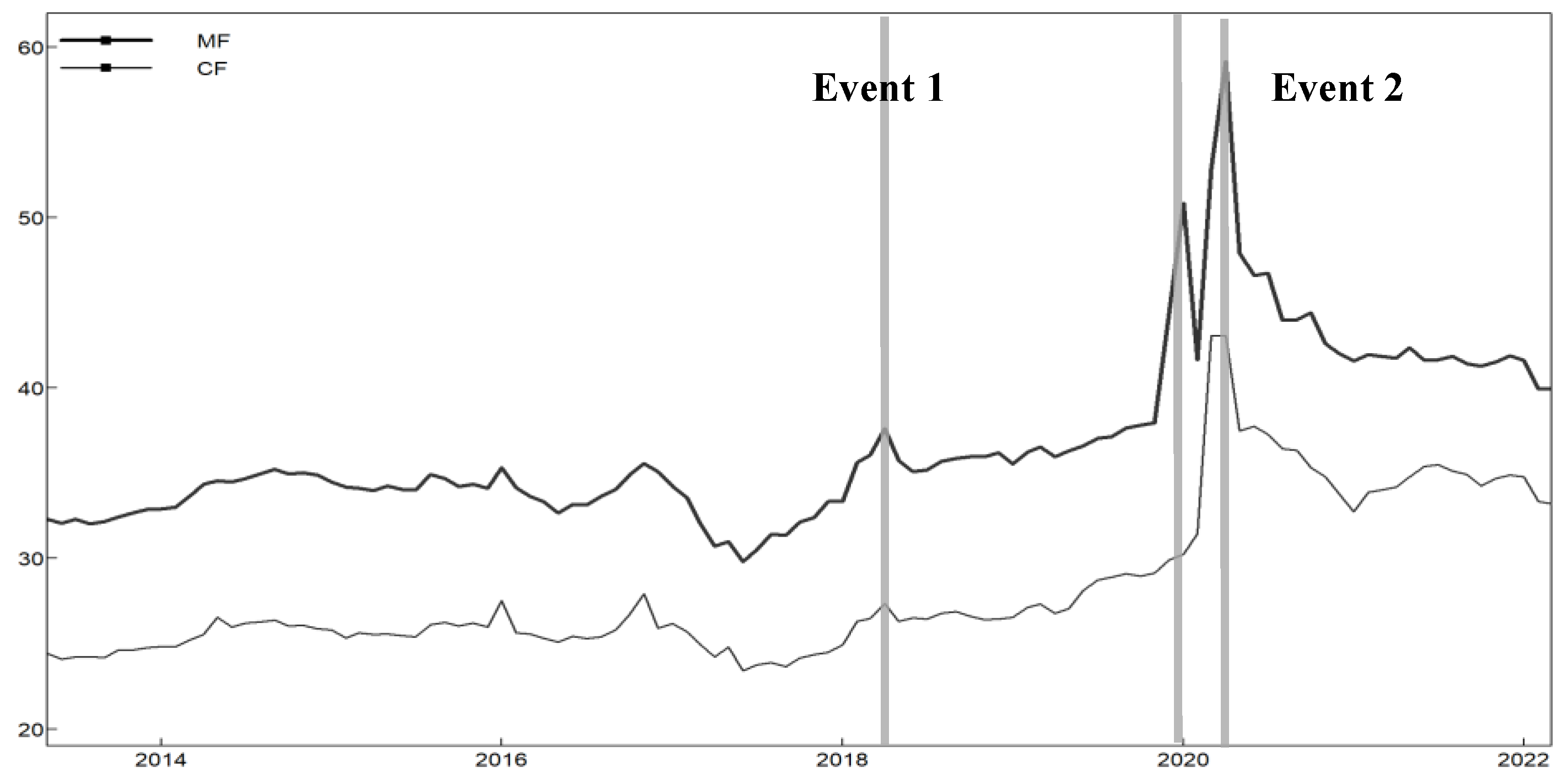
We further adopt a rolling window approach to calculate the dynamics of the total volatility spillover index under the mixed-frequency and common-frequency methods in the selected sample and analyze the time trend of the risk spillover effect. The results are shown in Figure 1, where the date of the horizontal axis is the end date of the rolling window.

As can be seen from Figure 1, the total volatility spillover index values for the mixed-frequency and the common-frequency methods are basically coincident over the full sample period, indicating that both methods can portray the risk contagion relationship between the commodity markets and the macroeconomy. However, the volatility spillover (thick line) for the mixed-frequency method is generally higher than that for the common-frequency method (thin line), with the mean value of the total volatility spillover index for the mixed-frequency method being 36.80, while the mean value of the total volatility spillover index for the common-frequency method is only 27.17. This suggests that using the common-frequency method to portray risk contagion underestimates the impact of the commodity markets on the macroeconomy by ignoring high frequency data.

The total volatility spillover index has obvious time-varying characteristics in the full sample period. Before 2018, the volatility spillover trend is generally relatively calm, but in early 2018 in China, “structural deleveraging” accelerated, money supply growth slowed down, and the credit policy was increasingly tight. The trade friction between China and the United States has further intensified the uncertainty of markets, with great downward pressure on the economy and the accumulation of financial risks. In 2018, the total external volatility spillover from the commodity markets rose by 2.51 compared with 2017, and the external volatility spillover from macroeconomic sectors such as loans and consumption also increased significantly; overall, the economy was generally stable in the late stage, basically achieving a new balance.

In early 2020, Chinese commodities prices showed V-shaped fluctuations due to the outbreak of the COVID-19 pandemic, and the risk contagion effect between the commodity markets and the macroeconomy was exacerbated by the sharp fluctuation in commodities prices. As can be seen from Figure 1, the total volatility spillover index has increased significantly since the outbreak of the COVID-19 pandemic, peaking at 59.16 in March 2020 and remaining at a high level, with an average total spillover index of 43.65 since the outbreak. This shows that the impact of COVID-19 on the risk contagion between commodity markets and the macroeconomy is significant and persistent compared with the economic downturn in 2018.

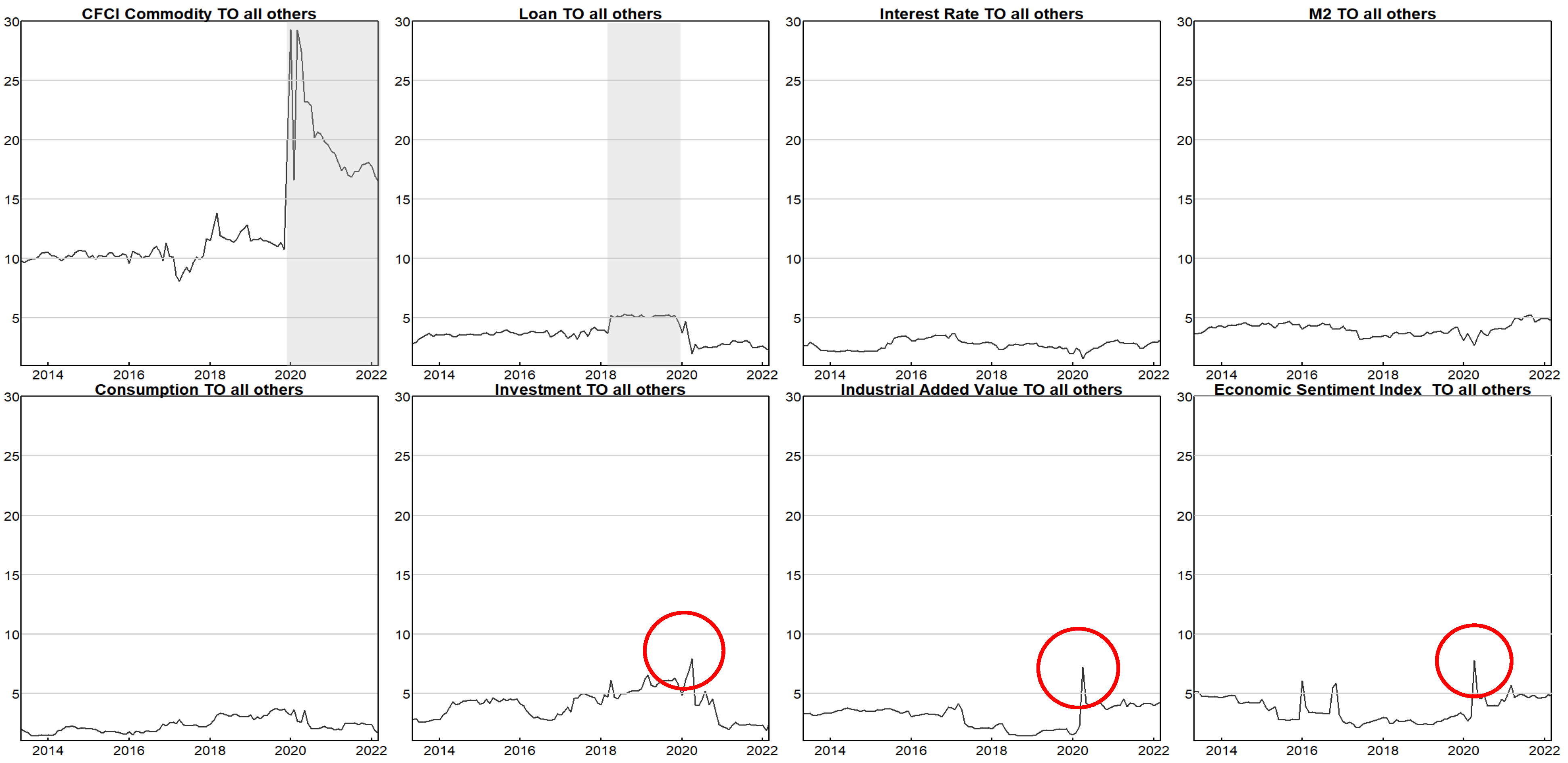
Next, we dynamically consider the rows and columns of Table 2 and observe the dynamics of the targeted volatility spillover. Figure 2 shows the dynamics of the sum of volatility spillovers from the CFCI commodity and macroeconomic sectors to all other sectors (corresponding to the “TO” row in Table 1).

As can be seen from Figure 2, the total volatility spillover from the CFCI commodity is the largest; the average value of the spillover index is 13.05; and the total volatility spillover from each macroeconomic sector is small, among which the spillover effect from investment and loans is relatively large. Loans have a phase of growth in 2018–2019, in which the average value of the total volatility spillover index rose by 1.26 compared with 2017. Due to the “structural deleveraging” policy, there existed a significant decline in new RMB loans from financial institutions, while China has gradually shifted from “deleveraging” to “stabilizing leverage” since the second quarter of 2018 in response to the dual challenges of economic downturn and trade friction, with annual loan growth in 2018 reaching a record high of 19.5%.

In January 2020, the sudden outbreak of the COVID-19 pandemic brought a sharp shock to the commodity markets, causing the CFCI commodity closing price to plummet from 164.9 to 140.7 during the first quarter of 2020, and the volatility spillover effect from the CFCI commodity also increased significantly, peaking at 29.31 in January. Commodities prices returned to their previous level in July and then showed a strong upward trend, with the CFCI commodity closing price peaking at 235.6 on October 19, 2021, and the total volatility spillover effect of the CFCI commodity also remaining high, with the average spillover index reaching 19.91. The total volatility spillover from investment, industrial added value, and the economic sentiment index all showed a small increase in March 2020, and the total volatility spillover from industrial added value and the economic sentiment index remained high in the later period, with a certain degree of risk resonance within the commodity markets. The risk level in the system has been greatly improved.

Figure 3 shows the dynamics of the total volatility spillover received by the CFCI commodity and macroeconomic sectors from all other sectors (corresponding to the “FROM” row in Table 1). It can be seen that the volatility spillover from external sources increased in early 2020, among which loans, interest rates, and M2 have fallen back significantly in the later period and the total volatility spillovers are lower than the original level; however, consumption, investment, industrial added value, and economic sentiment index have increased more and fallen back less in the later period, with the average value increasing by 1.88, 2.87, 3.04, and 1.53, respectively, compared with 2019. Next, we document the results of the dynamics of the net volatility spillover of the CFCI commodity and macroeconomic sectors in the selected sample interval in Figure 4.

As seen in Figure 4, the net external volatility spillover of the CFCI commodity is positive and dominates the risk contagion relationship within all sectors of the macroeconomy. The net external volatility spillover index surged from 18.00 to 27.32 in January 2020 due to the impact of the COVID-19 pandemic, and the average value during the pandemic rose by 7.69, or 76.4%, compared to 2019. Except for a slight increase in the economic sentiment index, all macroeconomic sectors show a negative peak in early 2020, with consumption and investment being more significantly affected by the impact of the COVID-19 pandemic and the net external volatility spillover index showing a significant decline, with the average value falling by 2.78 and 5.35, respectively, compared to 2019.

3.3. Analysis of Volatility Spillover Effects since the Outbreak of the COVID-19 Pandemic

With the global spread of the COVID-19 pandemic, commodities prices have fluctuated and market risks have increased dramatically. Therefore, this paper focuses on the impact of the sudden public event of the COVID-19 pandemic on the commodity markets and macroeconomic sectors by using a net risk spillover framework. We examine the risk contagion relationship between China’s commodity markets and macro sectors since the outbreak of the COVID-19 pandemic (since December 2019) using mixed-frequency and common-frequency methods, respectively, in

Table 3. Volatility spillover matrix since the outbreak of the COVID-19 pandemic.

		CFCI Commodity	Loans	Interest Rate	M2	Consumption	Investment	Industrial Added Value	Economic Sentiment Index	FROM
CFCI commodities	MF CF	42.74 24.17	7.79 15.40	6.47 6.20	14.34 4.90	9.76 19.38	4.86 9.23	5.01 4.32	9.02 16.41	57.26 75.83
Loans	MF CF	39.73 7.97	2.37 24.43	3.02 6.02	15.38 8.61	12.21 14.07	3.02 17.31	9.42 2.53	14.84 19.05	97.63 75.57
Interest Rate	MF CF	42.60 16.90	2.94 15.09	1.72 27.80	17.09 6.61	18.73 12.11	5.05 4.30	3.89 10.42	7.98 6.76	98.28 72.20
M2	MF CF	35.99 12.62	4.38 14.14	2.66 16.82	6.98 29.58	17.75 1.15	12.48 5.60	3.00 9.97	16.75 10.11	93.02 70.42
Consumption	MF CF	46.90 1.42	3.84 18.18	3.13 2.76	16.71 0.13	17.10 26.60	1.45 25.66	0.35 14.83	10.52 10.43	82.90 73.40
Investment	MF CF	39.89 12.45	1.40 15.70	3.14 7.88	14.30 8.99	18.49 10.78	3.34 18.16	7.27 10.65	12.16 15.38	96.66 81.84
Industrial Added Value	MF CF	32.95 8.32	1.41 15.74	4.89 2.95	4.38 2.38	16.76 21.84	7.57 14.07	9.08 19.98	22.95 14.72	90.92 80.02
Economic Sentiment Index	MF CF	46.44 15.31	5.32 14.35	3.93 2.15	18.25 0.51	12.39 24.70	1.43 5.09	3.04 7.48	9.20 30.40	90.80 69.60
TO	MF CF	284.51 74.99	27.09 108.61	27.25 44.79	100.45 32.12	106.09 104.04	35.87 81.25	31.98 60.20	94.22 92.86	707.46 598.87
NET	MF CF	227.26 −0.83	−70.53 33.05	−71.04 −27.41	7.44 −38.30	23.19 30.64	−60.79 −0.58	−58.94 −19.82	3.42 23.26	40.22% 12.52%

.

The difference between the volatility spillover matrices during the pandemic period and the full sample period is almost always positive, indicating that the volatility between the CFCI commodity and macroeconomic sectors and within the macroeconomic sectors increased significantly during the pandemic period, whether using the mixed-frequency or the common-frequency methods. Although the direction of volatility change is consistent for both methods, the growth of the external volatility spillover effect of the CFCI commodity is more significant under the mixed-frequency method, and the net volatility spillover of the CFCI commodity is in the opposite direction under both methods, which indicates that using the common-frequency method may cause significant bias in the conclusions and that the mixed-frequency method can more accurately portray the risk shock of China’s commodity markets to the macroeconomy during the period of the COVID-19 pandemic.

Table 3 shows that the CFCI commodity has significant risk spillovers to all macreconomic sectors during the pandemic, and its value range from 32.95 to 46.90, with strong net risk spillovers to consumption and economic sentiment index of 37.14 and 37.43, respectively. Volatility from the macroeconomic sectors has a small impact on the CFCI commodity, with volatility spillover ranging from 4.86 to 14.34. During this period, the total external volatility spillover of the CFCI commodity increased to 40.22% of the total systemic volatility spillover. The volatility spillover of the commodity markets has become the main cause of systemic risk contagion.

Within the macroeconomy, M2, consumption, and the economic sentiment index are the main exporters of risk contagion. This is due to the fact that consumer confidence in China was shaken during the COVID-19 pandemic and consumption slowed down severely, with total retail sales of consumer goods in China falling by 3.9% year-on-year in 2020. At the same time, with the significant stagnation of economic and social activities, China’s economic sentiment index also dropped below 90 for the first time in January–April 2020, and the economic operation continued to be under pressure. To cope with this downward pressure on the economy, the Chinese central bank implemented countercyclical adjustment through accommodative monetary policy, with a year-on-year growth rate of M2 reaching 11.1% in April 2020, a record high since 2017. The sharp fluctuations in M2, consumption, and the economic sentiment index have produced strong volatilities to loans and interest rates. The net volatility spillover of the three sectors to the rest of the macroeconomy reached 29.08, 60.33, and 40.85, respectively.

Based on these results, we conducted a network analysis of the net volatility spillover effects of the commodity markets interacting with the macroeconomic sectors over the full sample period and since the outbreak of the COVID-19 pandemic, and the results are shown in Figure 5.

Figure 5a shows that the volatility spillover network is sparse; the blue and orange lines are thin in the full sample period, while the volatility spillover network lines are significantly larger and thicker during the COVID-19 period, as seen in Figure 5b, indicating that the risk contagion effect from the commodity markets to the macroeconomic sectors and within the macroeconomic sectors increased significantly since the outbreak of the COVID-19 pandemic. The blue node for the CFCI commodity is the largest in both the full sample and the pandemic period and is the main exporter of risk. Among all the orange nodes in Figure 5b, M2, consumption, and the economic sentiment index have larger nodes and lines pointing to multiple markets such as investment, consumption, and industrial added value, indicating that M2, consumption, and the economic sentiment index are the main sources of risk contagion within the macroeconomy during the pandemic.

3.4. Impulse Analysis of the Commodity Markets on the Macroeconomy

Next, we investigate the impulse response of macroeconomic shocks caused by China’s commodity markets during the COVID-19 pandemic based on the factor-augmented vector autoregressive model.

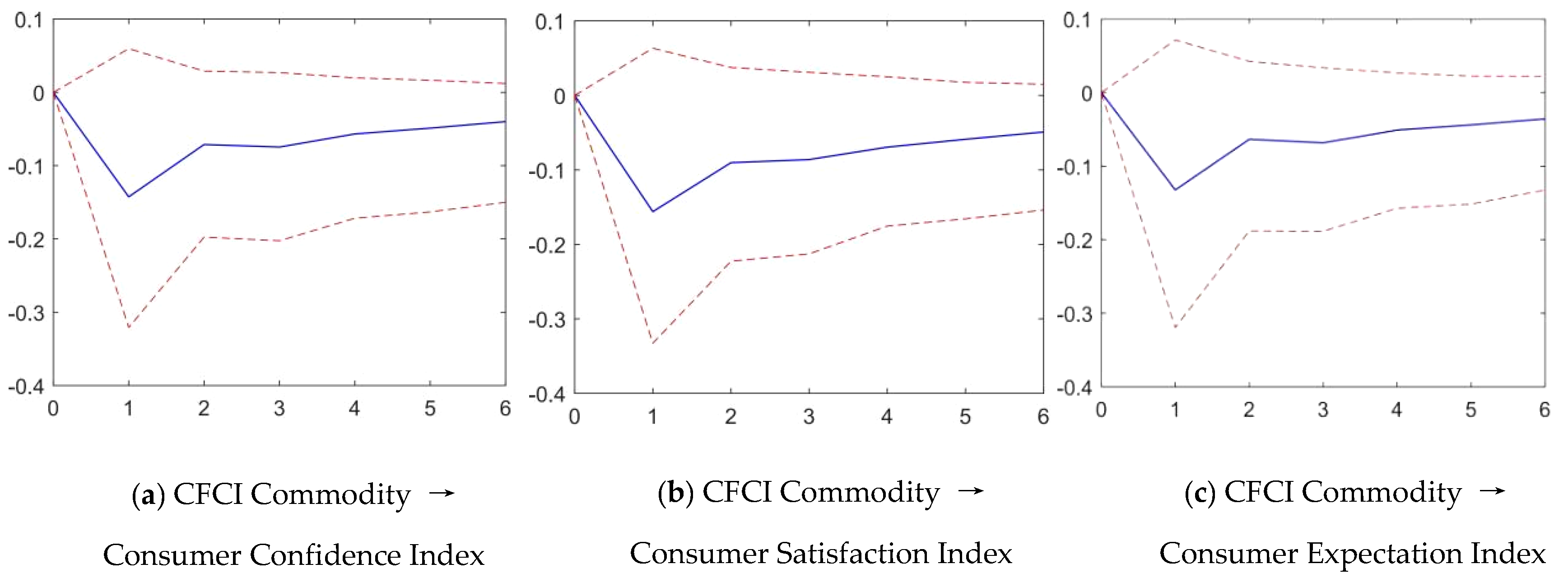
In Figure 6a–c, we can see that the consumer confidence index, satisfaction index, and expectation index reached a negative peak at 1 month after the impact occurred, with late rapid rebound, but were still slightly lower than before after six months. It shows that although the targeted policies and measures adopted at the beginning of the outbreak by China to maintain the stability of material supply and market prices worked in boosting consumer confidence, market confidence has not fully recovered to the original level.

From Figure 7a–c, it can be seen that the fluctuation of commodity markets at the beginning of the pandemic has a certain negative impact on the consumption of grain oil and food, automobiles, and clothing industries. Due to the impact of the COVID-19, consumers in China are paying more attention to health care and national fitness. From Figure 7d, we find that the consumption of sports and entertainment products in China showed a strong growth during the pandemic period.

Figure 8 shows that the CFCI commodity volatility during the COVID-19 pandemic caused negative shocks to investment sectors for a long time, and the adverse effects did not fully disappear until six months after the shock, which indicates that the violent volatility in commodity markets can cause investors’ market expectations to fall for a longer period of time and can cause increased uncertainty about the future and a significant weakening of investment intentions.

From Figure 9a,b, we find that during the pandemic, the volatility of commodity markets had a significant negative and positive impact on medium- and long-term loans and short-term loans and bill financing, respectively, which indicates that banks and other financial institutions are more inclined to cede their loan quota to more liquid short-term loans and to reduce long-term loans during the crisis, while the shrinkage of medium- and long-term loans will further inhibit investment, discourage consumption, and hinder domestic economic recovery. From Figure 9c,d, it can be seen that residential loans and loans to enterprises and institutions are subject to negative and positive shocks from the commodity markets, respectively, which indicates that the high volatility of commodities will have a significant negative spillover on residents’ consumption intentions by affecting the consumer prices, which in turn leads to a weakened demand for medium- and long-term consumer loans. While the credit pressure of many small and micro enterprises with weak risk resistance has increased due to the crisis, their demand for loans has been strengthened by monetary policies such as “refinancing and rediscounting” and “lowering of interest rates”.

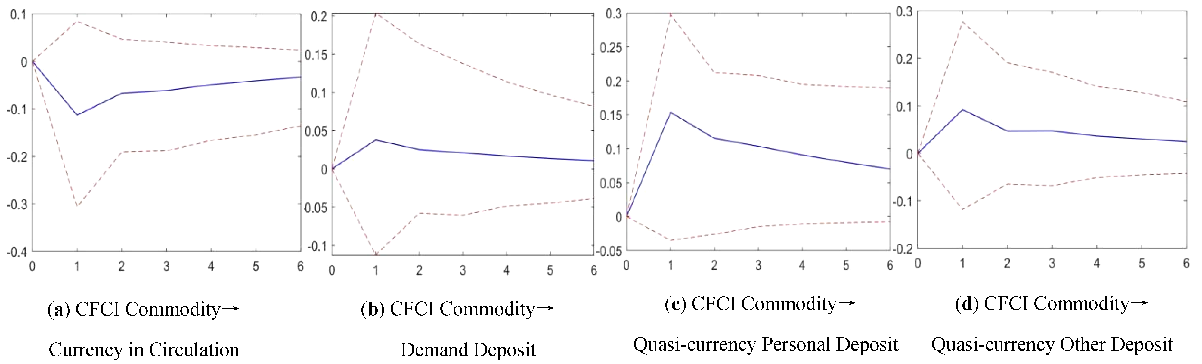
Figure 10a shows that China’s currency in circulation generally slowed down during the pandemic. The currency in circulation suffered a brief negative shock from the commodity markets, but the adverse impact was generally manageable. Meanwhile, Figure 10b–d show that all types of deposits received a brief positive shock at the beginning of the pandemic, with quasi-currency personal deposit receiving the sharpest shock, with a peak of 0.15. This suggests that the sharp fluctuations in the commodity markets will increase the propensity of micro-individuals to save and that enterprises and residents are more willing to deposit funds in banks during a crisis. The market activity and money liquidity will be reduced, which will restrict the rapid recovery and sustainable development of the national economy to a certain extent.

4. Analysis of Risk Spillover Contagion Mechanism

This paper further incorporates consumer confidence into the analytical framework and studies the contagion mechanism of risk spillovers between the commodity markets and macroeconomic sectors for the full sample.

Table 4. Mixed-frequency causal analysis of risk contagion for the full sample.

		CFCI Commodity	Loans	Interest Rate	M2	Consumption	Investment	Industrial Added Value	Consumer Confidence
CFCI Commodity	MF CF		0.00 *** 0.82	0.01 *** 0.73	0.00 ** 0.38	0.06 * 0.62	0.92 0.19	0.00 ** 0.35	0.08 * 0.72
Loans	MF CF	0.05 ** 0.27		0.12 0.45	0.02 ** 0.39	0.85 0.06 *	0.59 0.90	0.82 0.62	0.81 0.13
Interest Rate	MF CF	0.08 * 0.34	0.18 0.43		0.53 0.25	0.90 0.03 **	0.94 0.57	0.12 0.47	0.18 0.91
M2	MF CF	0.00 *** 0.12	0.07 * 0.18	0.06 * 0.04 **		0.74 0.12	0.92 0.87	0.10 * 0.14	0.00 *** 0.41
Consumption	MF CF	0.67 0.98	0.91 0.92	0.39 0.79	0.10 * 0.11		0.13 0.11	0.00 *** 0.84	0.00 *** 0.53
Investment	MF CF	0.04 ** 0.16	0.51 0.84	0.68 0.48	0.02 ** 0.04 **	0.67 0.99		0.33 0.56	0.66 0.63
Industrial Added Value	MF CF	0.03 ** 0.88	0.95 0.51	0.02 ** 0.01 **	0.39 0.72	0.97 0.19	0.19 0.22		0.27 0.99
Consumer Confidence	MF CF	0.52 0.80	0.00 *** 0.11	0.19 0.46	0.14 0.40	0.27 0.08 *	0.09* 0.19	0.07 * 0.45

¹ The p-values of the test statistics are reported in the table, and the original hypothesis is “no causality from column elements to row elements”; ² ***, **, * denote the rejection of “no Granger causality” at 1%, 5%, and 10% significance levels, respectively; ³ The lag order is 2, and the number of test repetitions N is 500.

shows that under the mixed-frequency approach, most macroeconomic sectors significantly reject the original hypothesis of “no Granger causality from the commodity market to the sector,” which indicates that the risk spillover from the commodity markets in China will cause direct shocks to macroeconomic sectors such as loans and interest rates. In addition, combining the causality within macroeconomic sectors, we find that the volatility of commodity markets has a direct impact on the smooth operation of macroeconomic sectors and an indirect impact on other macroeconomic sectors, such as consumption and consumer confidence through loan and money sectors. Table 4 also shows that there exists a causal relationship from most macroeconomic sectors to the commodity markets, which indicates that the commodity markets are subject to feedback shocks from the macroeconomy while causing risk shocks to the macroeconomic sectors. The risk contagion paths from the commodity markets to the macroeconomy are not accurately identified by using the traditional common-frequency method. Combining the results of causality analysis in Table 4, we further draw the corresponding risk spillover contagion mechanism in Figure 11.

Figure 11 shows that in addition to direct shocks to the investment sector, the risk spillover from the commodity markets is also reflected in indirect shocks to the consumption sector. The causal relationships of Commodity markets →Macroeconomic Sectors → Consumer Confidence → Commodity markets and Commodity markets → Macroeconomic Sectors → Consumption → Commodity markets suggest that macro environment changes such as output decline and credit crunch triggered by commodity market shocks will lower consumers’ economic expectations and cause significant shocks to the consumption sectors, which will further cause feedback shocks to the commodity markets by increasing economic uncertainty. At the same time, the causality of Commodity markets → M2 → Loans → Commodity markets under the expectation effect suggests that changes in monetary liquidity will increase banks’ risk expectations, forcing them to raise interest rates or reduce credit supply and increasing the uncertainty of funding costs [41]. In the context of volatile commodity markets, however, traders tend to raise their margins significantly to avoid trading risk, and changes in currency liquidity and credit market shocks further affect market participants’ cash flow expectations and increase their nervousness. There is also a causal relationship of Commodity markets →M2 → Investment, which suggests that macro uncertainty caused by changes in market liquidity affects investors’ investment expectations and creates a wait-and-see mentality, which is in line with the findings of Bloom (2009) [42].

In addition, the interest rate effects of Commodity markets → Interest Rate →Industrial Added Value → Commodity markets and Commodity markets → Interest Rate → M2 → Commodity markets in Figure 11 indicate that, under the risk shock from the commodity markets, shocks in the interbank lending market will lead to changes in monetary liquidity, which will increase financing costs and financial risks of industrial enterprises, depress the enthusiasm of production, and cause the output value of industrial enterprises to fall. The rising cost of funds and the downward pressure on the economy caused by them will further feed back to the commodity markets and intensify the volatility of the commodity markets. The common-frequency method cannot accurately identify the above risk contagion path.

5. Conclusions and Recommendations

This paper examined the risk contagion between China’s commodity markets and macroeconomic sectors from the perspective of volatility spillover by using mixed-frequency and common-frequency methods. It was found that the traditional common-frequency method has many biases in portraying the risk contagion relationship due to the neglect of high frequency data information and that the common-frequency causality test cannot accurately identify risk spillover contagion paths. Therefore, the findings of this paper were based on the MF-VAR model and mixed-frequency causality test.

The study found that China’s commodity markets were the net exporter of risk contagion and had significant shock effects on all sectors of the macroeconomy. Since the outbreak of the COVID-19 pandemic, the risk contagion effect between China’s commodity markets and the macroeconomy has increased significantly, with the commodity markets fluctuation generating negative shocks to the investment sector with a longer duration. This caused changes in macroeconomic sectors, such as reduced medium- and long-term loans, reduced currency circulation rate, and weakened individual consumption willingness, which further increased the downward pressure on the economy and held back economic recovery. The commodity markets have multiple paths of risk contagion, such as wealth effect, interest rate effect, and expectation effect. Commodity market fluctuation has a direct impact on loans, interest rates, M2, investment, and industrial added value, as well as indirect impacts on consumption and consumer confidence through the above variables. The fluctuations in macroeconomic sectors cause feedback shocks to the commodity markets through the contagion paths of Macroeconomic Sectors → Consumption → Commodity markets and M2 → Loans → Commodity markets.

Since serving the real economy is the vocation and purpose of finance, the complete description of the risk contagion between commodity markets and the macroeconomy in this paper can provide an important reference for the soundness of the existing systemic risk prevention system. The commodity markets are an important risk exporter. In the environment of the COVID-19 pandemic and intensified geopolitical conflicts, regulators should fully clarify the driving factors behind the commodities price fluctuations and prevent risk spillover by adjusting interest rates and taxes, optimizing import and export policies, and strengthening strategic reserves on the basis of establishing a sound price warning mechanism and enhancing market transparency. In addition, the risk spillover contagion mechanism shows that risk shocks from the commodity markets will accumulate through other macroeconomic sectors and eventually reverse back to the commodity markets. Therefore, regulators should be alert to abnormal fluctuations in the monetary and consumption sectors, strengthen monetary policy, and stabilize consumption fundamentals to block the indirect shock channels of risks. They should also strengthen guidance for loans and interest rates to efficiently meet credit demand, ensure the smooth operation of industrial enterprises, and prevent feedback shocks and multiple superimpositions of risks.