Article

Spatio-Temporal Network for Sea Fog Forecasting

1
School of Industrial and Management Engineering, Korea University, Seoul 02841, Republic of Korea
2
Underwater Survey Technology (UST) 21, Incheon 21999, Republic of Korea
3
Korea Hydrographic and Oceanographic Agency, Busan 49111, Republic of Korea
*
Author to whom correspondence should be addressed.
Sustainability 2022, 14(23), 16163; https://doi.org/10.3390/su142316163
Submission received: 2 November 2022 / Revised: 27 November 2022 / Accepted: 30 November 2022 / Published: 3 December 2022

Abstract

:
Sea fog can seriously affect schedules and safety by reducing visibility during marine transportation. Therefore, the forecasting of sea fog is an important issue in preventing accidents. Recently, in order to forecast sea fog, several deep learning methods have been applied to time series data consisting of meteorological and oceanographic observations or image data to predict fog. However, these methods only use a single image without considering meteorological and temporal characteristics. In this study, we propose a multi-modal learning method to improve the forecasting accuracy of sea fog using convolutional neural network (CNN) and gated recurrent unit (GRU) models. CNN and GRU extract useful features from closed-circuit television (CCTV) images and multivariate time series data, respectively. CCTV images and time series data collected at Daesan Port in South Korea from 1 March 2018 to 14 February 2021 by Korea Hydrographic and Oceanographic Agency (KHOA) were used to evaluate the proposed method. We compare the proposed method with deep learning methods that only consider temporal information or spatial information. The results indicate that the proposed method using both temporal and spatial information at the same time shows superior accuracy.

1. Introduction

Sea fog is an important atmospheric phenomenon generated by warm and humid air passing over the cold sea or cold air passing over the warm sea. It mainly occurs in July around the coast of South Korea. Sea fog causes low visibility, limiting various marine activities. In South Korea, marine accidents caused by sea fog account for 29.5% of all marine accidents. Thus, early forecasting of sea fog is essential in maritime safety and route management [1]. Traditionally, statistical and numerical analyses of sea fog occurrence are mostly used. However, numerical analysis currently used by the Korea Meteorological Administration is vulnerable to accurate meteorological forecasting due to climate change over time.
Numerical analysis predicts future weather using numerical calculations through meteorological observation, provided that dynamics and physical equations which govern atmospheric conditions and motion on Earth are sufficiently known [2]. The mesoscale model version 5 (MM5) used for numerical prediction is based on the Pennsylvania State University/National Center for Atmospheric Research model designed by Antes et al. [3] and has been improved and supplemented to suit the South Korea meteorological environment [4]. The MM5 predicts sea fog by substituting observation values into a predetermined coefficient as a three-dimensional primitive equation model. However, the method of substituting observations into a calculated equation cannot quickly represent changing weather conditions, and predicting sea fog in detail in time is a challenge.
It is possible to collect many observational data of various types with the recent development of meteorological observation equipment. Miao et al. [5] predicted fog through a deep learning method using time series meteorological data. However, because of the characteristic of the time series model, the longer the input data, the more information in front of the input data is lost. Consequently, the meteorological data do not change significantly over time, so it is difficult to improve the predictive performance.
In this study, we propose a spatio-temporal network for sea fog (STN-SF) forecasting. Our purpose is to accurately forecast sea fog that adversely affects marine transportation. To improve sea fog forecasting performance, we simultaneously use multivariate time series meteorological data and closed-circuit television (CCTV) images to reflect temporal and spatial information. The overall architecture of STN-SF consists of sequence-to-sequence (Seq2Seq) with attention [6] based on gated recurrent unit (GRU) cells [7]. In STN-SF with an encoder and decoder, the encoder sequentially receives information from CCTV images extracted from the convolutional neural network (CNN) and time series data and generates a context vector reflecting spatio-temporal information. Meanwhile, the decoder receives the context vector generated by the encoder as input and then forecasts sea fog. In particular, data augmentation techniques that can show distinct differences by modifying the texture of CCTV images were used to effectively extract spatial information regarding sea fog from the encoder. CCTV images collected by Korea Hydrographic and Oceanographic Agency (KHOA) at Daesan Port in South Korea from 1 March 2018 to 14 February 2021 and a meteorological time series public dataset from the Korea Meteological Administration (KMA) that matches the time of the CCTV images were used. Results show that the proposed method takes advantage of the complementary benefits by simultaneously using time series meteorological data and CCTV images and improves sea fog forecasting performance by applying data augmentation techniques.
The main contributions of this study can be summarized as follows:
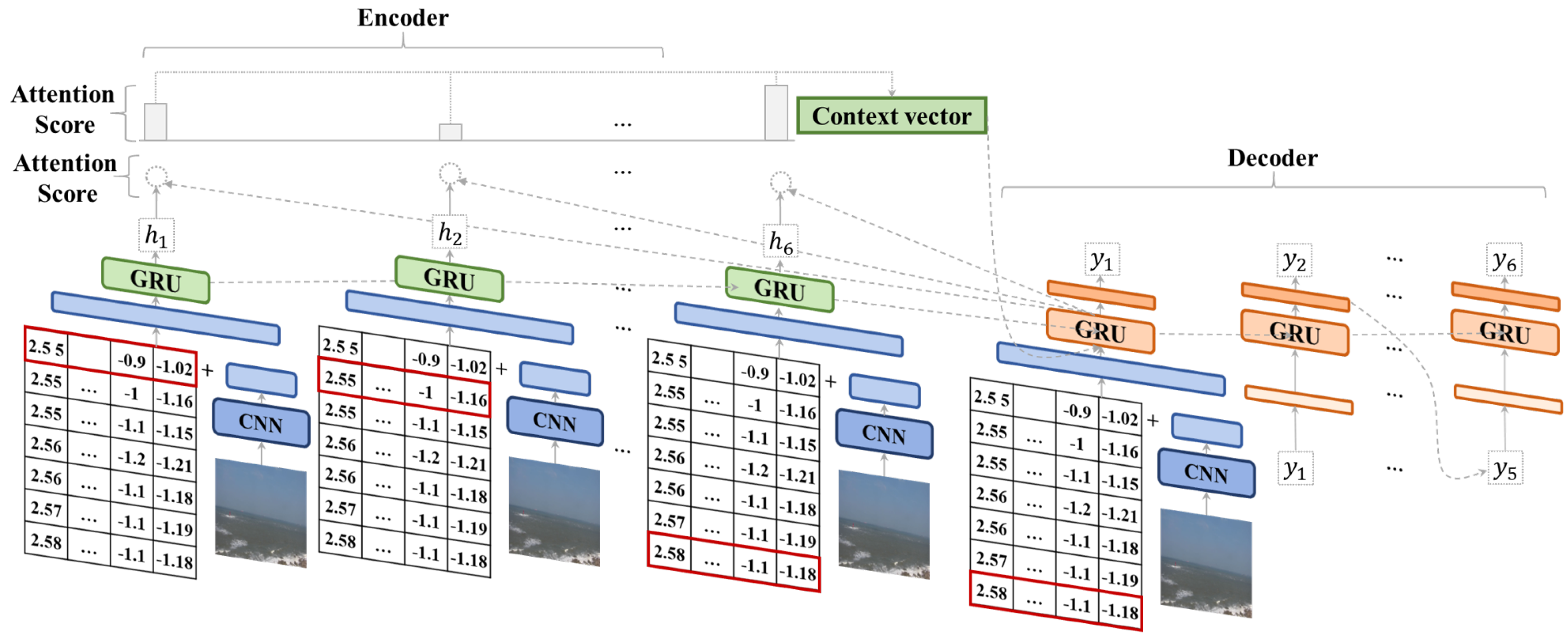
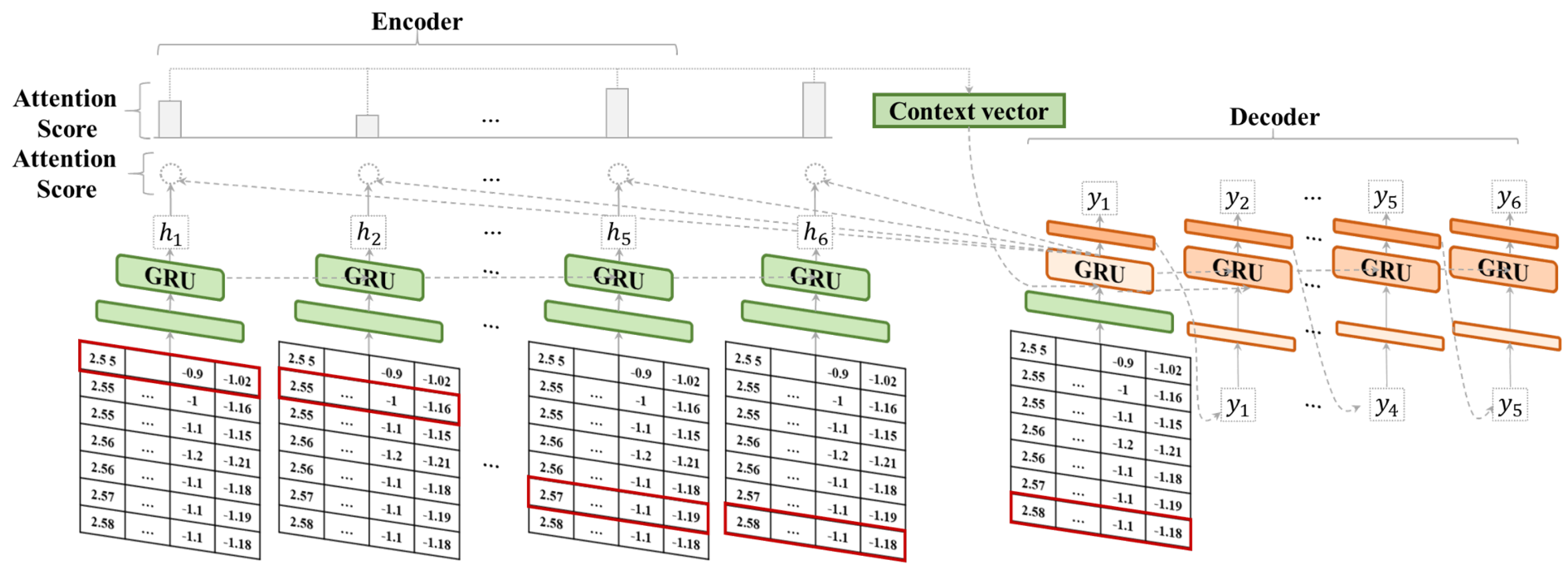
  • A spatio-temporal network for sea fog forecasting is proposed. The method aims to take advantage of the complementary benefits by simultaneously using time series meteorological data and CCTV images. To the best of our knowledge, this has not been previously studied in the field of fog forecasting.
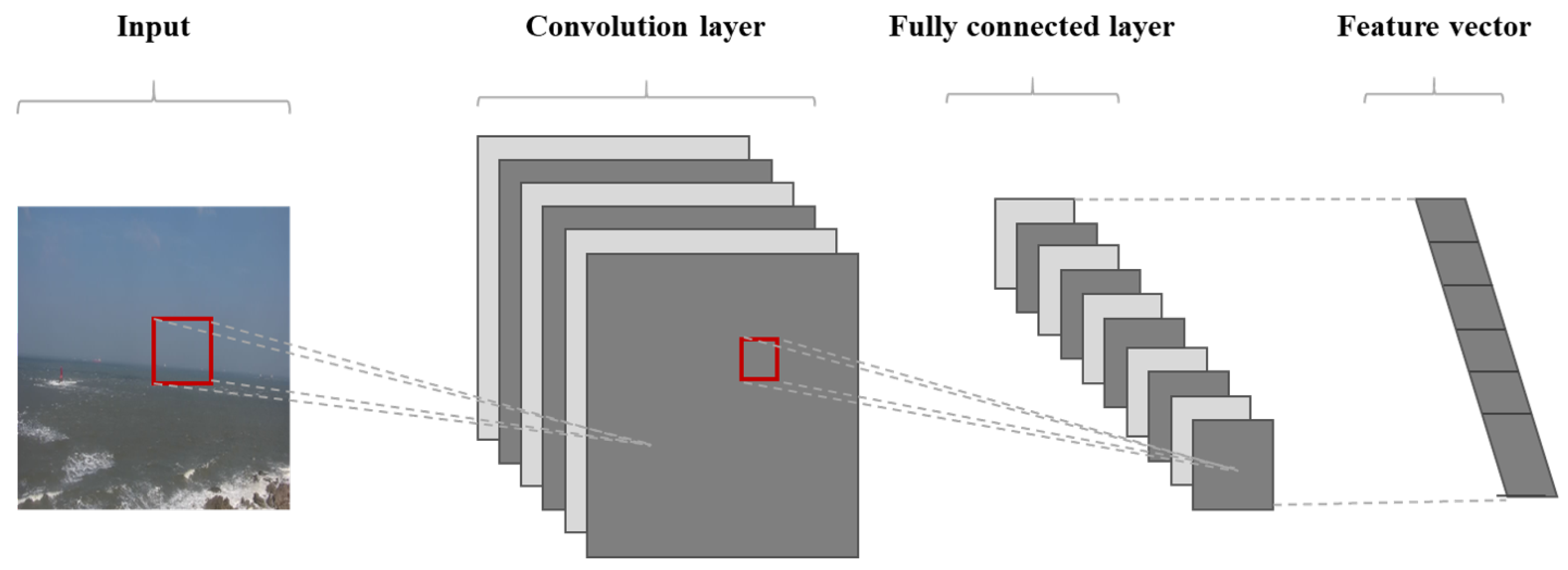
  • Data augmentation techniques were applied to the image. CCTV images contain information such as sea fog, sea, sky, and clouds. Data augmentation techniques modify the texture of the image to reveal distinct differences to effectively extract spatial information about sea fog.
  • Experiments on data augmentation techniques were conducted to improve the sea fog forecasting performance of the proposed method. An experiment was conducted by applying random invert, color jitter, Gaussian blur, random solarization, and random posterization, showing what augmentation techniques can effectively capture information about sea fog information.
The remainder of the paper is organized as follows. Section 2 reviews recent advances in a climate with artificial intelligence. Section 3 describes the details of the proposed method. Section 4 presents the experimental results and discussion. Section 5 gives the concluding remarks and future research directions.

2. Related Works

Heuristic algorithms or machine learning has been proposed to forecast fog (or sea fog). Dev et al. [8] proposed a heuristic algorithm based on meteorological variables to predict the occurrence of heavy fog. This algorithm is divided into test and check blocks with the threshold for each variable and makes the correct prediction when all thresholds are satisfied. Guijo-Rubio et al. [9] proposed a hybrid prediction model that adjusts the window size of the data according to the dynamics of the time series to predict daily low visibility events. Dewi et al. [10] used random forest (RF), gradient boosting machine (GBM), extreme randomized tree, and stacked ensemble to predict fog events at Wamena Airport in Indonesia. Han et al. [11] applied support vector machine (SVM) and ensemble-based machine learning methods to predict the fog dissipation problem occurring at Incheon Port and Haeundae Beach in South Korea. Castillo-Botón et al. [12] predicted the atmospheric low visibility by applying AdaBoost, GBM, and RF models to multivariate data composed of meteorological variables (temperature, pressure, humidity, visibility, and wind) in Mondonedo, Spain. However, these methods have difficulties in improving prediction performance because they cannot effectively handle meteorological information that changes over time.
Recently, deep learning methods have been used to address climate change problems. Son et al. [13] forecasted solar power generation using satellite imagery, a means to study and detect climate change. Guerra et al. [14] classified weather conditions based on three classes of weather images, namely, rain, snow, and fog. This method uses data augmentation techniques and CNNs that can effectively process images and classifies weather conditions through an SVM classifier. Pulukool et al. [15] applied CNN to meteorological observations to predict the occurrence of hail. Zhao et al. [16] proposed multi-task learning that can simultaneously process segmentation and weather classification tasks on weather cues, such as fog or clouds, to provide a comprehensive description of weather conditions. Dewi et al. [10] used an artificial neural network and meteorological data to predict the fog phenomenon at the airport. Han et al. [11] used a multi-layer perceptron and time series meteorological and oceanographic data to predict fog dissipation for Incheon port and Haeundae beach in South Korea. They also applied a recurrent neural network (RNN) to reflect meteorological information that changes over time, demonstrating the effectiveness in predicting fog dissipation. Zhao et al. [17] applied CNNs to classify fog levels for outdoor video based on three classes, namely, fog-free, mist, and dense fog. FogNet [18] uses a dense block-based 3D-CNN architecture to predict fog using complex meteorological data with 3D patterns. However, these methods make prediction using only a single image; thus, they could not consider temporal characteristics that frequently occur in fog prediction problems. Consequently, these methods are vulnerable to minute meteorological changes.
In recent deep learning research, multi-modal learning has been used to understand the characteristics of multiple data types, integrating them into a single piece of information. Ngiam et al. [19] proposed a multi-modal learning method based on a deep neural network to learn audio and video modalities. Wang et al. [20] proposed using a CNN-based multi-modal deep fusion method based on both typical and infrared image pairs to predict visibility, a measure of atmospheric transparency. Bijelic et al. [21] proposed a multi-modal learning method that fuses lidar, RGB, gated, and radar images collected from vehicle driving. This method effectively detects objects in autonomous vehicles using images taken in adverse weather, using lidar, radar, and gated near-infrared sensors. The multi-modal vehicle detection network (MVDNet) [22] leverages the complementary advantages of lidar and radar with multi-modal learning to accurately detect objects in foggy weather conditions that reduce visibility. Zhang et al. [23] proposed using CNN and transformer to handle spatial and temporal information of meteorological data. In the present study, we use a multi-modal learning framework that can take advantage of the complementary benefits between meteorological time series data and CCTV images.

3. Proposed Method

3.1. Data Acquisition

The purpose of our study is to forecast sea fog using multivariate time series meteorological data and CCTV images. Multivariate time series meteorological data were obtained from sensors installed around the lighthouse at Daesan Port (37 00 49 N, 126 25 14 E) in South Korea. CCTV images were obtained through video taken by a camera attached near the lighthouse. Time series data consist of meteorological data (air temperature, relative humidity, wind speed, and sea-level air pressure) and oceanographic data (water temperature) in one-minute increments. Minimum, maximum, mean, and standard deviation of the observations in 10 min increments were calculated so as to have data with 32 meteorological and oceanographic features. The images were extracted from CCTV videos and annotated with the help of experts for the presence or absence of sea fog. The dataset was divided into training, validation, and test sets. The training dataset contains 9178 observations from 1 March 2018 to 19 October 2019. The validation dataset contains 1000 observations from 11 November 2019 to 4 June 2020. The test dataset contains 2108 observations from 5 June 2020 to 14 February 2021.

3.2. Model Architecture and Data Augmentation Techniques

In this study, we propose the STN-SF using multivariate meteorological time series data and CCTV images to forecast sea fog. In STN-SF with the encoder and decoder, the encoder sequentially receives information from CCTV images extracted from the CNN and time series data and generates a context vector reflecting spatio-temporal information. Meteorological time series observations include tabular data with 10 min intervals. CCTV images are composed of parts in the video that match with the meteorological observation points. Figure 1 shows the overall architecture of the proposed STN-SF, consisting of an encoder−decoder of Seq2Seq with attention.
GRU cells [7] are used to reflect temporal information in the encoder and the decoder. The encoder generates a context vector containing spatio-temporal information by sequentially receiving vectors that combine CCTV images information extracted from the CNN and time series data. The decoder then receives the context vector generated by the encoder and spatio-temporal information and forecasts sea fog. In particular, data augmentation techniques that can show distinct differences by modifying the texture of CCTV images are used to effectively extract spatial information regarding sea fog from the encoder.
In the Seq2Seq with attention architecture, the encoder takes the input data in time order and compresses all data at the end into a single context vector. The context vector is then fed into the decoder that receives data from time points after the input data as start tokens and predicts future points sequentially. The attention mechanism is used to prevent loss of information in the first received data when taking input and output long-term data [6]. In the attention mechanism, whenever the decoding phase predicts a specific point in time, a different context vector is applied at each timestep instead of a single context vector that represents the input data. The attention mechanism is represented as follows:
s i j = s c o r e ( p i 1 , h j ) ,
a i j = s o f t m a x ( s i j ) ,
c i = j = 1 m a i j h j ,
p i = f ( p i 1 , y i 1 , c i ) ,
where p i 1 is the hidden state of the previous step used to predict the i t h data in the decoder. h j is the hidden state of the encoder, and s i j is the similarity score calculated through the dot product of p i 1 and h j . Equation (2) normalizes the probability by applying the softmax function to the score s i j as the attention weights a i j . The context vector c i is computed as the weighted sum of the hidden states h j and the attention weights a i j . A different value is input for each step of the decoder. Finally, in the decoder, to predict the next timestep, p i 1 is represented as Equation (4). p i 1 is the hidden state for predicting the next data through the hidden state p i 1 and data y i 1 of the previous step and the computed context vector c i . Fog is forecasted using a Seq2Seq structure with the attention mechanism applied to time series meteorological data. The encoder outputs a context vector with meteorological observations in six timesteps organized in 10 min intervals, and the decoder predicts the fog after 1 h. Figure 2 shows the Seq2Seq with attention architecture using meteorological time series data.
We consider spatial information as well as temporal information. In the encoder, CNN is used to extract CCTV images information. CNN consists of three main structures, namely, a convolution layer, a pooling layer, and a fully connected layer. In CNN, feature maps of the input image are generated by convolution layers, and feature information is compressed through pooling and fully connected layers. Figure 3 shows the CNN architecture using images. Various methods have been proposed for the CNN architecture. Representative CNN architectures include AlexNet [24], VGG16 [25], and ResNet [26]. In particular, this study uses VGG16, ResNet−18, and ResNet−50, which can effectively extract image features. In addition, pretrained CNN architectures are used with ImageNet, a vast dataset, when extracting feature vectors of sea fog images. Consequently, vectors that combine CCTV image information extracted from a pretrained CNN and meteorological time series data are processed to reflect spatio-temporal information in the encoder of Seq2Seq with attention.
The CCTV images used in this study include sea, sky, and clouds as well as sea fog. Sea fog occurs between the sea and the sky and resembles clouds. CNN architectures that process CCTV images can be confused by similar information when extracting feature vectors for sea fog. When sea fog information was extracted from CCTV images, it was determined that there will be performance changes depending on the image texture. Therefore, data augmentation techniques that can show a distinct difference by modifying the texture of an image are used to extract an accurate feature vector. The data augmentation techniques used in this study include random invert, color jitter, Gaussian blur, random solarization, and random posterization. Figure 4 shows images with data augmentation applied to the original image. As shown in Figure 4, some images to which data augmentation techniques have been applied have texture differences between fog, sea, sky, and clouds. The proposed method uses data augmentation techniques on CCTV images in the encoder while simultaneously utilizing the complementary advantages of meteorological time series data and CCTV image features to forecast sea fog.

4. Experimental Results

This study trained STN-SF consisting of CNN and RNN structures. In the encoder, we used ResNet−50, which is pretrained by the ImageNet dataset [27]. In the encoder and decoder, we used the GRU with Xavier weight initialization [28]. The proposed method was trained for 20 epochs with a batch size of 16. The parameters were optimized with the AdamW optimizer [29] using a learning rate of 0.001. The time length of the input data in the encoder is 1 h, and a total of six pieces of 10 min data were used. The decoder autoregressively infers the occurrence of sea fog at 10 min intervals until one hour. All experiments were implemented with a single NVIDIA TITAN RTX GPU with PyTorch 1.11.0.
The proposed method was compared with various machine learning and deep learning methods in the aspect of the unimodal method, including RF [30], light gradient boosting machines (LGBM) [31], GRU, and ResNet−50. RF and LGBM cannot effectively reflect the temporal characteristic of time series data. Therefore, for an equivalent comparison with the proposed method, time-lagged features at one hour behind at 10 min intervals were generated so that RF and LGBM could handle past information as well as present information. GRU can effectively reflect the temporal information of time series data. However, ResNet−50 reflects only spatial information of the image, not the temporal information. In the case of ResNet−50, only CCTV images were used to see if the presence of sea fog could be judged well. The GRU and STN-SF, considering temporal information, were trained to forecast sea fog one hour later using six observations at 10 min intervals as input data. RF and LGBM were trained based on the processed time-lagged data.
The performance was evaluated using specialized metrics in the field of sea fog forecasting, including accuracy, probability of detection (POD), success ratio (SR), and critical success index (CSI). These metrics are calculated using the confusion matrix presented in Table 1 containing the instances in the predicted and actual classes. Accuracy is the proportion of predicted successfully for either fog or no fog among the total number of predictions. POD is the proportion of fogs predicted successfully among the real fogs. SR is the proportion of fog predicted successfully among the predicted fogs. CSI is a balanced metric of POD and SR. Accuracy, POD, SR, and CSI can be calculated by the following equations:
Accuracy = H + C H + C + F + M ,
POD = H H + M ,
SR = H H + F ,
CSI = H H + F + M .
Table 2 shows the comparative results of sea fog forecasting models. STN-SF yielded the best result in terms of accuracy, SR, and CSI. For POD, ResNet−50 performed better than the proposed method but not a significant degree. RF and LGBM performed poorly on both datasets with and without historical information. This indicates that machine learning methods lack the ability to extract time series contexts. GRU, i.e., deep learning methods specialized for time series data, showed better performance than machine learning because it has strong ability to extract temporal information. ResNet−50, i.e., deep learning methods specialized for images, achieved good performance by using sea fog image. This indicates that sea fog image also has rich information for sea fog forecasting. Because STN-SF used both time series and image data, it showed the best performance among the comparative models. POD of ResNet−50 was good, but SR was relatively low. This demonstrated that STN-SF was better in CSI, reflecting the balance between POD and SR.
STN-SF uses a CNN architecture on CCTV images to extract features for sea fog. An experiment was conducted with VGG16, ResNet−18, and ResNet−50 to examine the performance impact with different CNN architectures. Table 3 shows the results of comparison experiments while changing the CNN architecture in STN-SF. The results showed that ResNet−50 produced better results than others although their differences are not significant.
The performance of CNN can be degraded by similar information when extracting feature vectors. The CCTV images contain sea fog information. When sea fog information is extracted from CCTV images, we hypothesize that more important information can be captured using augmentation techniques. Random solarization, Gaussian blur, random posterization, color jitter, and random invert techniques are used. Table 4 shows the performance results by applying various data augmentation techniques. Regardless of the CNN architecture, the performance was improved with augmentation. In terms of CSI, random posterization performed the best, implying that it can help effectively extract sea fog information.

5. Conclusions

In this study, we propose the STN-SF to forecast sea fog using both meteorological and oceanographic time series data, and CCTV images simultaneously. Our method takes advantage of the complementary benefits of temporal and spatial information. STN-SF consists of GRU-based Seq2Seq with attention and ResNet−50. In particular, spatio-temporal information is simultaneously reflected in the encoder of STN-SF by extracting spatial information of CCTV images from ResNet−50 and extracting temporal information from meteorological and oceanographic data. Moreover, the performance is further improved by using data augmentation techniques that can show distinct differences by modifying the texture of CCTV images to effectively extract spatial information about sea fog. Real data collected from Daesan Port in South Korea are used, and sea fog is forecasted one hour later using six observations at 10 min intervals as input data. Results show that the proposed method is superior in terms of various metrics by using time series meteorological data and CCTV images simultaneously to take advantage of the complementary benefits and apply data augmentation techniques.
Our study can be extended in new directions in terms of the architecture of forecast models that reflect spatio-temporal information. The Seq2Seq with attention architecture used in this study does not effectively reflect the information of the previous time, as the time length of the input data is longer, and parallel processing is impossible. Transformer [32] using the self-attention mechanism is widely used in time series forecasting as a method to solve the above problems. Therefore, extending to transformer to input and output long-term data may be advantageous for new and fog forecasting studies. A more accurate forecasting will be possible if data augmentation techniques that can better reflect the texture in the image from a spatial point of view are considered. In future work, we hope to develop a method to improve sea fog forecasting performance by considering transformer and suitable data augmentation techniques. In addition, since we used data collected over three years, we will additionally collect and test time series meteorological data and CCTV images to prevent overfitting.

Author Contributions

Conceptualization, Y.T.K., J.H.H., K.J.K. and S.B.K.; methodology, J.P., Y.J.L., Y.J. and J.K.; investigation, J.P., Y.J.L., Y.J., J.K. and S.B.K.; data curation, J.H.H., K.J.K. and Y.T.K.; writing—original draft preparation, J.P., Y.J.L., Y.J. and J.K.; writing—review and editing, Y.J.L., Y.T.K. and S.B.K.; supervision, S.B.K. All authors have read and agreed to the published version of the manuscript.

Funding

This research was supported by Korea Hydrographic and Oceanographic Agency (Tender notice of Busan Regional Public Procurement Service: 2021031390600), Brain Korea 21 FOUR, the Ministry of Science and ICT (MSIT) in Korea under the ITRC support program supervised by the IITP (IITP-2020-0-01749), and the National Research Foundation of Korea grant funded by the Korea government (RS-2022-00144190).

Data Availability Statement

The data presented in this study are not publicly available due to privacy and legal restrictions.

Conflicts of Interest

The authors declare no conflict of interest.

References

  1. Heo, K.Y.; Park, S.; Ha, K.J.; Shim, J.S. Algorithm for sea fog monitoring with the use of information technologies. Meteorol. Appl. 2014, 21, 350–359. [Google Scholar] [CrossRef]
  2. Wang, S.; Li, H.; Zhang, M.; Duan, L.; Zhu, X.; Che, Y. Assessing Gridded Precipitation and Air Temperature Products in the Ayakkum Lake, Central Asia. Sustainability 2022, 14, 10654. [Google Scholar] [CrossRef]
  3. Anthes, R.A.; Warner, T.T. Development of hydrodynamic models suitable for air pollution and other mesometerological studies. Mon. Weather Rev. 1978, 106, 1045–1078. [Google Scholar] [CrossRef]
  4. Han, K.K.; Kim, Y.C. Numerical forecasting of sea fog at West sea in spring. J. Korean Soc. Aviat. Aeronaut. 2006, 14, 94–100. [Google Scholar]
  5. Miao, K.c.; Han, T.t.; Yao, Y.q.; Lu, H.; Chen, P.; Wang, B.; Zhang, J. Application of LSTM for short term fog forecasting based on meteorological elements. Neurocomputing 2020, 408, 285–291. [Google Scholar] [CrossRef]
  6. Bahdanau, D.; Cho, K.; Bengio, Y. Neural machine translation by jointly learning to align and translate. arXiv 2014, arXiv:1409.0473. [Google Scholar]
  7. Chung, J.; Gulcehre, C.; Cho, K.; Bengio, Y. Empirical evaluation of gated recurrent neural networks on sequence modeling. arXiv 2014, arXiv:1412.3555. [Google Scholar]
  8. Dev, K.; Nebuloni, R.; Capsoni, C. Fog prediction based on meteorological variables—An empirical approach. In Proceedings of the 2016 International Conference on Broadband Communications for Next Generation Networks and Multimedia Applications (CoBCom), Graz, Austria, 14–16 September 2016; IEEE: Hoboken, NJ, USA, 2016; pp. 1–6. [Google Scholar]
  9. Guijo-Rubio, D.; Gutiérrez, P.; Casanova-Mateo, C.; Sanz-Justo, J.; Salcedo-Sanz, S.; Hervás-Martínez, C. Prediction of low-visibility events due to fog using ordinal classification. Atmos. Res. 2018, 214, 64–73. [Google Scholar] [CrossRef]
  10. Dewi, R.; Harsa, H.; Prawito. Fog prediction using artificial intelligence: A case study in Wamena Airport. In Proceedings of the Journal of Physics: Conference Series; IOP Publishing: Bristol, UK, 2020; Volume 1528, p. 012021. [Google Scholar]
  11. Han, J.H.; Kim, K.J.; Joo, H.S.; Han, Y.H.; Kim, Y.T.; Kwon, S.J. Sea Fog Dissipation Prediction in Incheon Port and Haeundae Beach Using Machine Learning and Deep Learning. Sensors 2021, 21, 5232. [Google Scholar] [CrossRef]
  12. Castillo-Botón, C.; Casillas-Pérez, D.; Casanova-Mateo, C.; Ghimire, S.; Cerro-Prada, E.; Gutierrez, P.; Deo, R.; Salcedo-Sanz, S. Machine learning regression and classification methods for fog events prediction. Atmos. Res. 2022, 272, 106157. [Google Scholar] [CrossRef]
  13. Son, Y.; Yoon, Y.; Cho, J.; Choi, S. Cloud Cover Forecast Based on Correlation Analysis on Satellite Images for Short-Term Photovoltaic Power Forecasting. Sustainability 2022, 14, 4427. [Google Scholar] [CrossRef]
  14. Guerra, J.C.V.; Khanam, Z.; Ehsan, S.; Stolkin, R.; McDonald-Maier, K. Weather Classification: A new multi-class dataset, data augmentation approach and comprehensive evaluations of Convolutional Neural Networks. In Proceedings of the 2018 NASA/ESA Conference on Adaptive Hardware and Systems (AHS), Edinburgh, UK, 6–9 August 2018; IEEE: Hoboken, NJ, USA, 2018; pp. 305–310. [Google Scholar]
  15. Pulukool, F.; Li, L.; Liu, C. Using deep learning and machine learning methods to diagnose hailstorms in large-scale thermodynamic environments. Sustainability 2020, 12, 10499. [Google Scholar] [CrossRef]
  16. Zhao, B.; Hua, L.; Li, X.; Lu, X.; Wang, Z. Weather recognition via classification labels and weather-cue maps. Pattern Recognit. 2019, 95, 272–284. [Google Scholar] [CrossRef]
  17. Zhao, X.; Jiang, J.; Feng, K.; Wu, B.; Luan, J.; Ji, M. The Method of Classifying Fog Level of Outdoor Video Images Based on Convolutional Neural Networks. J. Indian Soc. Remote Sens. 2021, 49, 2261–2271. [Google Scholar] [CrossRef]
  18. Kamangir, H.; Collins, W.; Tissot, P.; King, S.A.; Dinh, H.T.H.; Durham, N.; Rizzo, J. FogNet: A multiscale 3D CNN with double-branch dense block and attention mechanism for fog prediction. Mach. Learn. Appl. 2021, 5, 100038. [Google Scholar] [CrossRef]
  19. Ngiam, J.; Khosla, A.; Kim, M.; Nam, J.; Lee, H.; Ng, A.Y. Multimodal deep learning. In Proceedings of the International Conference on Machine Learning (ICML), Bellevue, WA, USA, 28 June–2 July 2011. [Google Scholar]
  20. Wang, H.; Shen, K.; Yu, P.; Shi, Q.; Ko, H. Multimodal deep fusion network for visibility assessment with a small training dataset. IEEE Access 2020, 8, 217057–217067. [Google Scholar] [CrossRef]
  21. Bijelic, M.; Gruber, T.; Mannan, F.; Kraus, F.; Ritter, W.; Dietmayer, K.; Heide, F. Seeing through fog without seeing fog: Deep multimodal sensor fusion in unseen adverse weather. In Proceedings of the IEEE/CVF Conference on Computer Vision and Pattern Recognition, Seattle, WA, USA, 14–19 June 2020; pp. 11682–11692. [Google Scholar]
  22. Qian, K.; Zhu, S.; Zhang, X.; Li, L.E. Robust multimodal vehicle detection in foggy weather using complementary lidar and radar signals. In Proceedings of the IEEE/CVF Conference on Computer Vision and Pattern Recognition, Nashville, TN, USA, 20–25 June 2021; pp. 444–453. [Google Scholar]
  23. Zhang, X.; Jin, Q.; Yu, T.; Xiang, S.; Kuang, Q.; Prinet, V.; Pan, C. Multi-modal spatio-temporal meteorological forecasting with deep neural network. ISPRS J. Photogramm. Remote Sens. 2022, 188, 380–393. [Google Scholar] [CrossRef]
  24. Krizhevsky, A.; Sutskever, I.; Hinton, G.E. Imagenet classification with deep convolutional neural networks. Commun. ACM 2017, 60, 84–90. [Google Scholar] [CrossRef] [Green Version]
  25. Simonyan, K.; Zisserman, A. Very deep convolutional networks for large-scale image recognition. arXiv 2014, arXiv:1409.1556. [Google Scholar]
  26. He, K.; Zhang, X.; Ren, S.; Sun, J. Deep residual learning for image recognition. In Proceedings of the IEEE Conference on Computer Vision and Pattern Recognition, Las Vegas, NV, USA, 27–30 June 2016; pp. 770–778. [Google Scholar]
  27. Deng, J.; Dong, W.; Socher, R.; Li, L.J.; Li, K.; Fei-Fei, L. Imagenet: A large-scale hierarchical image database. In Proceedings of the 2009 IEEE Conference on Computer Vision and Pattern Recognition, Miami, FL, USA, 22–24 June 2009; IEEE: Hoboken, NJ, USA, 2009; pp. 248–255. [Google Scholar]
  28. Glorot, X.; Bengio, Y. Understanding the difficulty of training deep feedforward neural networks. In Proceedings of the Thirteenth International Conference on Artificial Intelligence and Statistics, JMLR Workshop and Conference Proceedings, Sardinia, Italy, 13–15 May 2010; pp. 249–256. [Google Scholar]
  29. Loshchilov, I.; Hutter, F. Decoupled weight decay regularization. arXiv 2017, arXiv:1711.05101. [Google Scholar]
  30. Breiman, L. Random forests. Mach. Learn. 2001, 45, 5–32. [Google Scholar] [CrossRef]
  31. Ke, G.; Meng, Q.; Finley, T.; Wang, T.; Chen, W.; Ma, W.; Ye, Q.; Liu, T.Y. Lightgbm: A highly efficient gradient boosting decision tree. In Proceedings of the Advances in Neural Information Processing Systems 30 (NIPS 2017), Long Beach, CA, USA, 4–9 December 2017; Volume 30. [Google Scholar]
  32. Vaswani, A.; Shazeer, N.; Parmar, N.; Uszkoreit, J.; Jones, L.; Gomez, A.N.; Kaiser, Ł.; Polosukhin, I. Attention is all you need. In Proceedings of the Advances in Neural Information Processing Systems 30 (NIPS 2017), Long Beach, CA, USA, 4–9 December 2017; Volume 30.
Figure 1. Overall architecture of the STN-SF.
Sustainability 14 16163 g001
Figure 2. Application of the attention mechanism to the Seq2Seq architecture of the encoder−decoder structure. The encoder receives a continuous input of time series data and produces a context vector. The decoder uses a different computed context vector for prediction for each timestep.
Sustainability 14 16163 g002
Figure 3. CNN architecture for extracting features from images. In the convolution layer, a feature map is generated through a compound multiplication operation and a slide of the input image. The information on the image is then compressed through the pooling process in the pooling layer, and the feature vector is finally generated through the fully connected layer.
Sustainability 14 16163 g003
Figure 4. Examples of various data augmentation techniques that can transform the texture of the original image.
Sustainability 14 16163 g004
Table 1. Confusion matrix for sea fog forecasting. Each column indicates the instances in a predicted class, and each row represents the instances in an actual class.
PredictionNo Fog Fog 
Real
No FogTrue Negative (C)False Positive (F)
FogFalse Negative (M)True Positive (H)
Table 2. Performance results of STN-SF and comparative methods. Unlike STN-SF considering all spatio-temporal information, the rest of the methods considered only one of the two. RF, LGBM, and GRU used meteorological and oceanographic tabular data in a time series, and ResNet−50 used sea fog image data. STN-SF used both tabular and image data. (* indicates using time-lagged features as historical information).
ModelsAccuracyPODSRCSI
RF0.6090.5530.6920.443
RF *0.5810.4550.6960.380
LGBM0.6080.5190.7080.427
LGBM *0.6040.5000.7130.416
GRU0.5680.8560.5790.528
ResNet−500.7150.9080.6870.642
STN-SF
(Proposed)
0.7990.8860.7850.713
Table 3. Performance of the proposed STN-SF with different CNN architectures.
ModelsAccuracyPODSRCSI
VGG160.7850.8420.7910.688
ResNet−180.7930.8330.8060.694
ResNet−500.7990.8860.7850.713
Table 4. Comparative results with different augmentation techniques. The best-performing augmentation techniques for each CNN architecture are shown in bold.
Encoder ArchitectureModelsAccuracyPODSRCSI
VGG16Random solarization0.7840.8440.7880.687
Gaussian blur0.7720.8650.7640.682
Random posterization0.7850.8420.7910.688
Color jitter0.7410.9190.7080.667
Random invert0.5980.9940.5850.583
No augmentation0.7110.9190.6690.632
ResNet−18Random solarization0.7760.8890.7570.691
Gaussian blur0.7830.8280.7950.683
Random posterization0.7930.8330.8060.694
Color jitter0.7730.8900.7520.688
Random invert0.6050.9890.5890.585
No augmentation0.7780.8760.7640.689
ResNet−50Random solarization0.7960.8810.7830.709
Gaussian blur0.7950.8930.7770.711
Random posterization0.7990.8860.7850.713
Color jitter0.7870.8860.7700.701
Random invert0.6560.9870.6230.618
No augmentation0.7840.8730.7730.695
Publisher’s Note: MDPI stays neutral with regard to jurisdictional claims in published maps and institutional affiliations.

