Probabilistic Forecasting for Demand of a Bike-Sharing Service Using a Deep-Learning Approach

Abstract

Efficient and sustainable bike-sharing service (BSS) operations require accurate demand forecasting for bike inventory management and rebalancing. Probabilistic forecasting provides a set of information on uncertainties in demand forecasting, and thus it is suitable for use in stochastic inventory management. Our research objective is to develop probabilistic time-series forecasting for BSS demand. We use an RNN–LSTM-based model, called DeepAR, for the station-wise bike-demand forecasting problem. The deep-learning structure of DeepAR captures complex demand patterns and correlations between the stations in one trained model; therefore, it is not necessary to develop demand-forecasting models for each individual station. DeepAR makes parameter forecast estimates for the probabilistic distribution of target values in the prediction range. We apply DeepAR to estimate the parameters of normal, truncated normal, and negative binomial distributions. We use the BSS dataset from Seoul Metropolitan City to evaluate the model’s performance. We create district- and station-level forecasts, comparing several statistical time-series forecasting methods; as a result, we show that DeepAR outperforms the other models. Furthermore, our district-level evaluation results show that all three distributions are acceptable for demand forecasting; however, the truncated normal distribution tends to overestimate the demand. At the station level, the truncated normal distribution performs the best, with the least forecasting errors out of the three tested distributions.

1. Introduction

Bike-sharing services (BSSs) have been widely used in many cities around the world to reduce carbon emissions and energy consumption and provide social benefits. BSSs also function as first- and last-mile transportation systems, which can work in conjunction with current motorized public systems, such as buses and subways. Hence, BSSs have attracted large numbers of city dwellers as well as visitors and are recognized as a sustainable and easy-access mode of transportation.

BSS operating systems are either dock-based or free floating. In a dock-based BSS (DBSS), users pick up a bike at one station and return it to another—that is, pick-up and return are only allowed at stations built in designated areas in the city. A free-floating BSS (FBSS) does not have stations, and users pick up nearby bikes and return them anywhere.

Essentially, a BSS requires bike redistribution (rebalancing) to increase the utilization of their assets (bikes) because it is a one-way rental service. As a DBSS has stations in fixed locations, and the service operator redistributes the bikes based on demand forecasting for each individual station. FBSS rebalancing is conducted on a regional basis. In Seoul city, FBSSs are generally employed for electric bikes or scooters, and the service area is restricted; therefore, less rebalancing is needed. In our paper, we focus on DBSS bike-demand forecasting. Forecasting is key to the success of bike rebalancing [1,2,3].

When the bikes need to be redistributed, a truck picks up surplus bikes from a station and delivers some of them to stations where there are not enough bikes for the upcoming demand. The truck traverses the area and continues its rebalancing work several times a day while considering cost-efficient routing. Therefore, bike rebalancing is a mix of inventory-management and vehicle-routing problems. To determine the appropriate number of bikes to be picked up and delivered, a forecast of the station-level demand for the bikes is necessary; therefore, knowing the probabilistic distribution of demand, particularly under high levels of uncertainty, is useful for making optimal decisions regarding the number of bikes placed in a station.

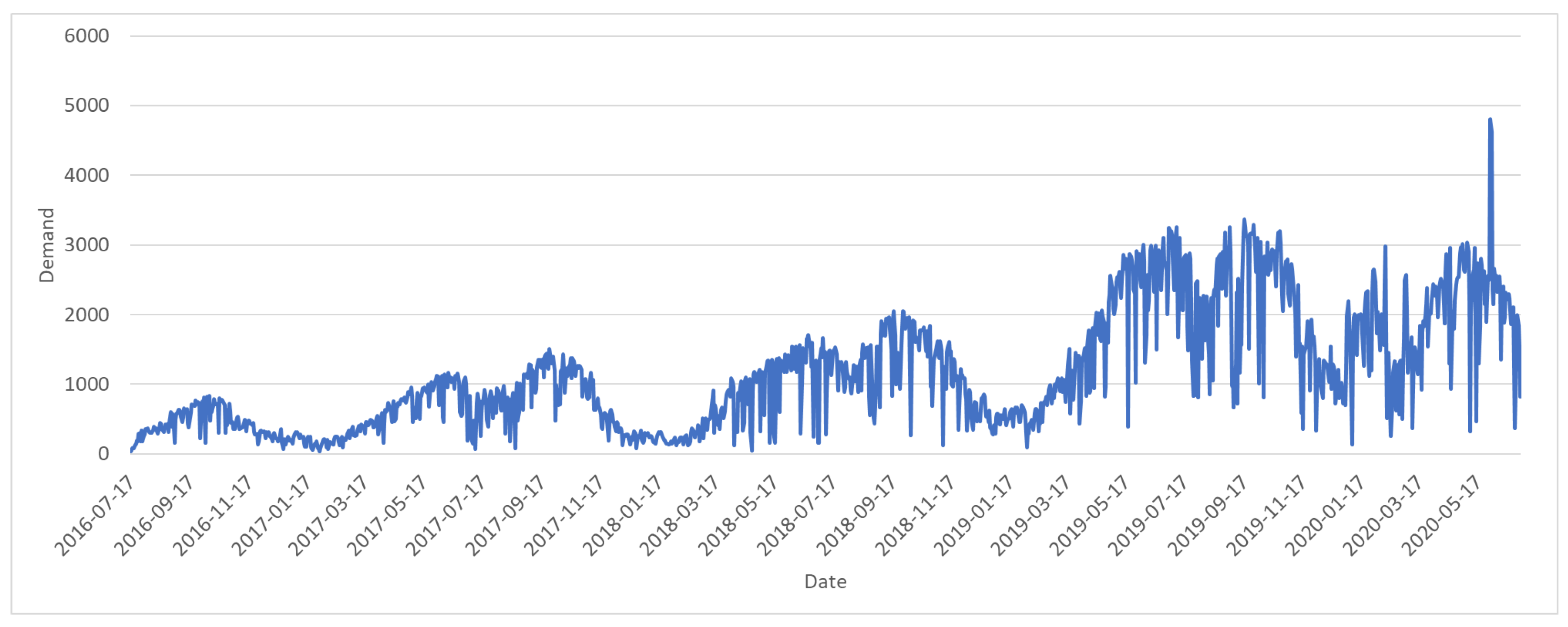
The demand for BSS has seasonal characteristics. Figure 1 displays variations of the daily bike demand over almost two years in the Dongdaemun-gu area of Seoul city. As the service year extends, more user demand occurs and, at the same time, there are seasonal demand fluctuations because biking is an outdoor activity that depends on weather conditions. Generally, the bike demand decreases substantially in the winter time and on hot summer days. Demand is also affected by everyday weather conditions, such as rain and snow. Therefore, we must consider seasonal and daily conditions when forecasting bike demand.

Figure 1. The daily bike demand for Dongdaemun-gu in Seoul.

Statistical time-series models using the state–space modeling (SSM) approach [4,5] learn patterns, such as trends and seasonality, and provide corresponding error terms that are used to compute prediction intervals; that is, SSM can provide a framework for distributional time-series forecasts. However, is difficult to infer shared patterns across the series using SSM because the model parameters are estimated independently for each bike station.

Consequently, demand forecasting is primarily for bike rebalancing, and the demand forecast must be obtained from all the city’s stations or at least from a city district. Individually developing SSM for each station within the entire area requires too many computations; therefore, it is difficult to consider this method a viable option. Moreover, demand correlations exist between neighboring stations [1,6]. For example, if one station is crowded with people picking up bikes, the nearby stations will be crowded with people from the same group. Therefore, we must consider alternative forecasting methodologies that encompass these issues.

Recently published research investigated deep-learning neural-network models that tackle time-series forecasting problems [7,8,9,10,11]. Despite the drawbacks of the deep-learning structure, such as requiring a great deal of data to obtain an accurate model and difficulty in interpreting the developed model, it can capture complex seasonality and trend patterns and incorporate sharing information across the time series into the model [7,9]. This is a purely data-driven modeling process that does not require labor-intensive human effort in raw data pre-processing and model-feature selection.

Time-series forecasting predicts the future value (or values) given individual or sequences of past entities. Among advanced deep-neural-network models, recurrent neural networks (RNNs) have been widely used for sequence modeling, such as natural language processing [12], and even in forecasting problems [7,9,10]. LSTM (long short-term memory) cells are also adopted to incorporate data with long time dependencies to the conventional RNN. The RNN model with LSTM cells (RNN-LSTM) has advantages when dealing with long-time sequential-history time series in forecasting.

Our research objective is to develop probabilistic time-series forecasting for bike-sharing-service demand. We use an RNN-LSTM model to resolve the station-wise bike-demand forecasting problem. Salinas et al. [7] provided a framework for probabilistic time-series forecasting that shared information across the time series—they called it DeepAR. DeepAR is based on an auto-regressive recurrent neural network with LSTM cells. They estimated parameters for the probabilistic distribution of target values in the prediction range using RNN-LSTM modeling.

The model learns one global model from time-series sales data in an online marketplace. Sales-item demand is correlated, showing common seasonal behaviors and sharing the same information represented by model covariates. Their model has similar problem structures compared to ours. There are many bike stations that are correlated in demand, and probabilistic forecasting is required to properly manage inventory through rebalancing. Therefore, we implement the DeepAR framework to the station-wise probabilistic bike-demand forecasting problem.

The output of DeepAR in this research is probabilistic distributions of bike demand for all the stations of a district (or the whole service area). Knowing the probabilistic distributions, as aforementioned, is essential to determine the optimal number of bikes required. To the best of our knowledge, this is the first approach to make the probabilistic forecasting for demand distributions of the stations of which demand is correlated in some ways, and this work can be a basis for the inventory rebalancing problem of BSS.

The rest of the paper is organized as follows: Section 2 reviews the related literature. Section 3 defines our demand-forecasting model based on DeepAR. Section 4 implements the model developed in Section 3 and provides the results of numerical experiments. The conclusions and future directions of our research are discussed in Section 5.

2. Related Work

Probabilistic demand forecasting provides decision makers with a set of information regarding uncertainties in the demand prediction. In the literature, we found that there are two representations of probabilistic forecasting [9]: the parametric and non-parametric models. In the former, a particular probability distribution is determined first, and the distribution parameters are estimated accordingly. In the non-parametric model, there is no pre-defined distribution, and an empirical distribution, usually defined by quantiles, is obtained from the prediction.

Snyder et al. [13] developed a methodology on prediction distribution and its performance measures. They used the Poisson and negative binomial distributions to develop a plan for inventory management. Salinas et al. [7] mainly employed the parametric model and used the parameterized Gaussian and negative binomial distributions for multiple time series of customer demand. Toubeau et al. [9] adopted their methodology in both of the models to provide probabilistic forecasting in electric power markets.

The literature [8,10,14,15,16] also suggests methodologies for probabilistic forecasting with a non-parametric structure. Some researchers believe that non-parametric methods are more robust because they does not rely on a pre-determined probability distribution [9]. Moreover, in a practical forecasting setting, a specified distribution will likely not fit the real data. However, parametric model predictions provide more information on the uncertainty in upcoming events if any dataset statistically fits to a particular probability distribution. Thus, it is easier to make a managerial decision on inventory control based on the probability distribution obtained from the forecasting.

Time series of counts occur frequently in a variety of supply chain operations. ARIMA (Auto-Regressive Integrated Moving Average) and exponential smoothing (ES) are a family of state-space models that have been widely employed for time-series forecasting. In the state-space model [4,5,13,14,16], there is a latent state that evolves over time and, thus, catches the time-series characteristics.

We believe that the real observation is solely governed by a corresponding latent state for that particular time, while the observation itself is assumed to be independent from others. The state-space model, including the ARIMA and ES, usually contains normality assumptions in the error term, and the model is essentially structured with real numbers. However, large divisions in demand forecasting applications have skewed non-negative data [14,16]; moreover, sometimes there are many zeros, which does not literally mean that the real count is zero but larger than zero (e.g., out of stock) or with small integers and/or little history. Thus, a complementary or alternative method is required.

Chapados [14] proposed a hierarchical probabilistic state–space model for predictions on a group of time series that share some common information. Their model adopted explanatory variables to impose time-dependent dynamics on the latent variable and some higher hierarchy variables explain the shared information. Seeger et al. [16] presented a robust and scalable forecasting algorithm that manipulates a generalized linear model (GLM) and exponential smoothing time series.

The GLM explains medium-to-longer-term variations of data, which separates the counts of zero, one, and larger with its latent variable. The time-series smoothing provides the short-term series predictions and temporal correlations. They used maximum-likelihood learning for their model parameters and provided a probabilistic forecast. They insisted that the model can efficiently handle thousands of items, which outperforms [14]; however, their paper did not tackle the information-sharing issue in a group of data.

Time-series data in supply-chain applications typically have Gaussian assumption violations that encompass intermittent, very small (near zero) and bursty counts in addition to non-negativity and non-linearity structures over time. Therefore, neural-network (NN) models are widely employed and easily found in the literature [7,8,10,17,18]. Researchers have argued that NN models are more flexible for forecasting because they require neither rigid structures nor data assumptions [17,18].

Kourentzes [18] proposed an NN model for intermittent time-series data, which captures dynamic demand rates over time and considers interactions between non-zero demand and the inter-arrival rate of demand events. The model is an expansion from Croston’s [19] method and its variants. However, the model did not outperform Croston’s method in terms of forecasting errors, although the model showed better performance than the benchmarks considering the inventory metrics point of view (service levels represented by holding and backlog volumes); therefore, Kourentzes insisted on the possibility of using the NN models in the intermittent time-series data.

Wen et al. [10] used a recurrent neural network (RNN) model with LSTM cells to perform probabilistic multi-period forecasting. The time series have recursive structures and often have long-term time dependencies, such as a year. Many NN-forecasting studies [7,8,9,10] have used RNN with LSTM cells. Wen et al. [10] adopted a Sequence-to-Sequence (Seq2Seq) framework with their innovative forking-sequences-scheme, which captures time-dependent features to perform multi-horizon forecasting with less errors caused by the RNN structure in the prediction period.

Thus, when multi-horizon values are predicted, the regular RNN scheme iteratively estimates one-step ahead of future values ($\widehat{y_{t+1}}$) given a predicted $\widehat{y_t}$. This process is likely to accumulate errors. The forking-sequences scheme works as a decoder in the prediction phase and, thus, avoids a prediction-dependent multi-horizon.

Wen et al. [10] performed forecasting for multiple time-series groups that shared information. This is similar to Rangapuram et al. [8] and Salinas et al. [7]. Rangapuram et al. combined the state–space model (SSM) and RNN to predict multiple time series in an information-sharing group. Their RNN network was used to compute the parameters for the SSM, which was followed by learning the shared network parameters. Salinas et al. [7] adopted an auto-regressive recurrent neural-network model with LSTM cells for probabilistic forecasting—they called the methodology DeepAR. DeepAR provides probabilistic forecasting for multiple time series.

Parameterized negative binomial and normal distributions are used for the forecasts, and the model predicts the parameters for the probability distributions for each time step in the forecasting horizon. DeepAR is able to provide quantile forecasts using Monte-Carlo sampling from the predicted probability distributions. As the model learns global seasonality and dependencies on given covariates from related time series, the authors argued that the DeepAR can handle group-dependent complexity from data, such as different magnitudes of counts. DeepAR also provides forecasts for items with little or no history in the information-sharing group.

Recent studies have widely used machine-learning methodologies for bike-sharing-system demand prediction [1,20,21,22]. Gao and Chen [20] applied linear regression, k-nearest neighbors, random forest, and support vector machine (SVM) methods to predict customer demand for bike-sharing systems. Explanatory features, such as the weather, COVID-19, air pollution, and social economic factors were incorporated into the prediction model, and they showed that random forest and support vector machine models were acceptable with weather and COVID-19 as the primary features.

In a similar study, Sathishkumar et al. [21] compared linear regression, gradient boosting machine (the best performer from their paper), SVM, boosted tree, and extreme gradient-boosting tree methods with a bike-sharing dataset from the same city in a different time period.

Lin et al. [1] used a graph convolution neural-network model with a data-driven graph filter (GCNN-DDGF) to provide station-level demand forecasting in a bike-sharing system in New York City. The model learns spatio-temporal dependencies between bike stations without elaborately pre-processing demand data. They compared six GCNN models (two with data-driven filters and the other four with pre-defined adjacency data, such as the spatial distance, demand, average trip duration, and demand correlation) and seven benchmark models. Their results showed that their proposed GCNN-DDGF with a recurrent block from long short-term memory (LSTM) architecture outperformed the others in terms of the prediction accuracy.

Mehdizadeh and Morency [22] adopted a hybrid convolutional neural network (CNN) and LSTM model to provide short-term bike-demand forecasts. The stations were grouped by their connection strength, which was defined by the number of trips within each group, and they predicted the demand for each group over the next 15 min. Compared with a typical ARIMA model, their proposed model performed better when measured by MAE and RMSE.

However, the forecasts we obtained from this paper are point estimates, and the forecasts’ usabilities and point estimations are limited in environments with uncertainties. The major role of forecasts in a bike-sharing system is to develop a bike-rebalancing plan. As there are many human-related uncertainties in the system, probabilistic forecasting is able to provide more information for decision makers.

As described, there is a large volume of literature on forecasting customer demand. In addition, as shared bike system services extend in many cities worldwide, bike-demand forecasting has been commonly studied in the literature. This paper is about bike-demand forecasting for the BSS and as with the bike-rebalancing problem, a probabilistic forecasting problem for bike demand is tackled. We selected a probabilistic forecasting methodology (DeepAR [7]) from the literature, as DeepAR can provide probabilistic distributions for the demand, and we applied it to a BSS.

3. Demand Forecasting Model

Denote a value from the time series for a station i by $z_{i,t}$. The conditional distribution is defined as $P\left({\mathbf{z}}_{i,t_0:T}\right|{\mathbf{z}}_{i,1:t_0-1})$ of time series ${\mathbf{z}}_{i,t_0:T}=[z_{i,t_0},z_{i,t_0+1},\dots ,z_{i,T}]$ given time series ${\mathbf{z}}_{i,1:t_0-1}=[z_{i,1},z_{i,1},\dots ,z_{i,t_0-1}]$ where $t_0$ stands for the first time point of the prediction period. Therefore, ${\mathbf{z}}_{i,1:t_0-1}$ is the past time range—the so-called “conditioning range”; and ${\mathbf{z}}_{i,t_0:T}$ is the future time range—in other words, the “prediction range”.

As DeepAR is an LSTM-based model, DeepAR requires an encoder–decoder structure. In DeepAR, encoder and decoder lengths reflect the length of the conditioning and prediction ranges, respectively. Both ranges have to be in the past to train the network so that all observations can be fed in for learning. When predicting, observations are used for the conditioning range.

An auto-regressive recurrent network is the base of our model [7,23]. We assume that a product of likelihood values makes up the model distribution as below.

$$\begin{array}{cc}\hfill Q_{\Theta }\left({\mathbf{z}}_{i,t_0:T}|{\mathbf{z}}_{i,1:t_0-1}\right)& =\prod _{t=t_0}^T{Q}_{\Theta }\left(z_{i,t}|{\mathbf{z}}_{i,1:t_0-1}\right)\hfill \\ \hfill & =\prod _{t=t_0}^{T}p\left(z_{i,t}|\theta ({\mathbf{h}}_{i,t},\Theta )\right)\hfill \end{array}$$

(1)

where ${\mathbf{h}}_{i,t}$ is an output of a function implemented by a recurrent neural network (RNN) with LSTM cells parameterized by $\Theta$; in other words, ${\mathbf{h}}_{i,t}=h\left({\mathbf{h}}_{i,t-1},z_{i,t-1},\Theta \right)$. Our model has characteristics that feed both the observation at the previous time point ($z_{i,t-1}$) and the output of the function, (${\mathbf{h}}_{i,t-1}$) in the sense of an auto-regressive feature. The conditional probability $p\left(z_{i,t}|\theta ({\mathbf{h}}_{i,t},\Theta )\right)$ is a fixed distribution parameterized by the function $\theta ({\mathbf{h}}_{i,t},\Theta )$ of ${\mathbf{h}}_{i,t}$, and the parameters of LSTM cells ($\Theta$. ${\mathbf{h}}_{i,t_0-1}$) carry information—the so-called context of observations in the conditioning range (${\mathbf{z}}_{i,1:t_0-1}$) to the prediction range.

We used the same LSTM models for both the conditioning and prediction range. This corresponds to the encoder–decoder scheme in a sequence-to-sequence model. The initial state for the decoder ${\mathbf{h}}_{i,t_0-1}$ is acquired by ${\mathbf{h}}_{i,t}=h\left({\mathbf{h}}_{i,t-1},z_{i,t-1},\Theta \right)$ for $t=1,\dots ,t_0-1$, and we observe demands for $t=1,\dots ,t_0-1$. For the encoder, the initial states ${\mathbf{h}}_{i,0}$ and ${\mathbf{z}}_{i,0}$ are set to zero by default.

With the model parameter $\Theta$, we obtained the joint samples ${\tilde{z}}_{i,t_i:T}\sim Q_{\Theta }\left({\mathbf{z}}_{i,t_0:T}|{\mathbf{z}}_{i,1:t_0-1}\right)$ by ancestral sampling. Once ${\mathbf{h}}_{i,t}$ is calculated over $t=1,\dots ,t_0-1$, ${\tilde{z}}_{i,t_i:T}\sim p\left(·\left|\theta \right({\tilde{\mathbf{h}}}_{i,t},\Theta )\right)$ are sampled over $t=1_0,\dots ,T$ when ${\tilde{\mathbf{h}}}_{i,t}=h\left({\mathbf{h}}_{i,t-1},{\tilde{z}}_{i,t-1},\Theta \right)$ with the initial states ${\tilde{\mathbf{h}}}_{i,t_0-1}={\mathbf{h}}_{i,t_0-1}$ and ${\tilde{z}}_{i,t_i:T}=z_{i,t_0-1}$. In this manner, we could compute the various quantiles of the demand distribution for the prediction period using samples obtained from the model.

3.1. Likelihood Models

Equation (1) embeds likelihood factor $p\left(z\right|\theta )$. With $p\left(z\right|\theta )$, the statistical properties of the data should be considered. In our model, a vector of parameters, $\theta$, of the probability distribution is predicted by the neural network for the following time period. For example, $\theta =[\mu ,\sigma ]$ is predicted when the normal distribution of the demand is assumed.

We evaluate three probability distributions for the experiments. They are normal (or Gaussian), truncated normal, or negative binomial likelihoods for real, positive real, or positive discrete number data, respectively. The probability distribution of the collected data is any distribution that positively describes the data. We attain parameters of a normal distribution $\theta =[\mu ,\sigma ]$ for a normal likelihood by using the affine function of the network output for $\mu$, in addition to the softplus activation function of the network output, $\sigma$, to ensure that the standard deviation is positive (Equation (2)). Thus,

$$\begin{array}{cc}\hfill & p_N\left(z\right|\mu ,\sigma )=\frac{1}{\sigma \sqrt{2\pi }}{e}^{-\frac{1}{2}{\left(\frac{z-\mu }{\sigma }\right)}^2}\hfill \\ \hfill & \mu \left({\mathbf{h}}_{i,t}\right)={\mathbf{w}}_{\mu }^T{\mathbf{h}}_{i,t}+b_{\mu }\hfill \\ \hfill & \sigma \left({\mathbf{h}}_{i,t}\right)=log\left(1+e^{{\mathbf{w}}_{\sigma }^T{\mathbf{h}}_{i,t}+b_{\sigma }}\right)\hfill \end{array}$$

(2)

In the case of a truncated normal likelihood, we use similar parameters to “parent” the general normal distribution of $\overline{\mu }$ and $\overline{\sigma }$ for the mean and variance, respectively. We use parameters of $z_{lb}=0$ and $z_{ub}=\infty$ for the lower and upper bounds of z, respectively, to specify the truncation interval. For a truncated normal likelihood, we attain the parameters of the truncated normal distribution $\theta =[\overline{\mu },\overline{\sigma }]$ by using the affine function of the network output for $\overline{\mu }$, in addition to the softplus activation function of the network output, $\overline{\sigma }$, to ensure that the standard deviation is positive as in Equation (3):

$$\begin{array}{cc}\hfill & p_{T}N\left(z\right|\overline{\mu },\overline{\sigma },0,\infty )=\frac{\frac{1}{\overline{\sigma }\sqrt{2\pi }}{e}^{-\frac{1}{2}{\left(\frac{z-\overline{\mu }}{\overline{\sigma }}\right)}^2}}{1-{\int }_{-\infty }^0\frac{1}{\overline{\sigma }\sqrt{2\pi }}{e}^{-\frac{1}{2}{\left(\frac{t-\overline{\mu }}{\overline{\sigma }}\right)}^2}dt}\hfill \\ \hfill & \overline{\mu }\left({\mathbf{h}}_{i,t}\right)={\mathbf{w}}_{\mu }^T{\mathbf{h}}_{i,t}+b_{\mu }\hfill \\ \hfill & \overline{\sigma }\left({\mathbf{h}}_{i,t}\right)=log\left(1+e^{{\mathbf{w}}_{\sigma }^T{\mathbf{h}}_{i,t}+b_{\sigma }}\right)\hfill \end{array}$$

(3)

We also observe the case of a negative binomial likelihood. The negative binomial distribution is widely used to model and depict the behavior of demand [24]. The negative binomial distribution is parameterized by the mean $\mu \in {\mathbb{R}}^{+}$ and shape $\alpha \in {\mathbb{R}}^{+}$. To ensure both parameters ($\mu$ and $\alpha$) are positive real numbers, we apply the softplus activation function on the output of the network (Equation (4)). The variance of the negative binomial distribution can be determined by $Var\left(z\right)=\mu +{\mu }^2\alpha$, where $\mu$ is the mean and $\alpha$ is the shape.

$$\begin{array}{cc}\hfill & p_{N}B\left(z\right|\mu ,\alpha )=\frac{\mathsf{\Gamma }(z+\frac{1}{\alpha })}{\mathsf{\Gamma }(z+1)\mathsf{\Gamma }\left(\frac{1}{\alpha }\right)}{\left(\frac{1}{1+\alpha \mu }\right)}^{\frac{1}{\alpha }}{\left(\frac{\alpha \mu }{1+\alpha \mu }\right)}^z\hfill \\ \hfill & \mu \left({\mathbf{h}}_{i,t}\right)=log\left(1+e^{{\mathbf{w}}_{\mu }^T{\mathbf{h}}_{i,t}+b_{\mu }}\right)\hfill \\ \hfill & \alpha \left({\mathbf{h}}_{i,t}\right)=log\left(1+e^{{\mathbf{w}}_{\alpha }^T{\mathbf{h}}_{i,t}+b_{\alpha }}\right)\hfill \end{array}$$

(4)

3.2. Training

Consider a dataset ${\left\{{\mathbf{z}}_{i,1:T}\right\}}_{i=1,\dots ,N}$ in the form of a time series. Our model learns the parameters $\mathsf{\Phi }$, which include the RNN $h(·)$ and $\theta (·)$ by maximizing the log-likelihood function. As a likelihood function in our study is a product of probabilities, the likelihood function is log-transformed for ease of the implementation and computation of the network’s loss function.

$$\mathcal{L}=\sum _{i=1}^N\sum _{t=t_0}^{T}logp\left(z_{i,t}|\theta \left({\mathbf{h}}_{i,t}\right)\right)$$

(5)

The computation of $\mathcal{L}$ in Equation (5) is straightforward because ${\mathbf{h}}_{i,t}$ is a deterministic function for its input; therefore, we can obtain all of the values. Moreover, it is possible for us to optimize Equation (5) by computing the stochastic gradient descent with respect to $\Theta$. Each time series created from the dataset is generated by choosing a time series with a different starting period. In our experiment, we created a time series of length T and divided it into conditioning and prediction ranges with certain ratios. For example, one of our datasets ranges from 19 September 2015 to 30 June 2020. We generated the first time series from $t=1$, which corresponds to 19 September 2019, and the second from $t=1$, which corresponds to 20 September 2019, and then we continued this procedure. The coverage of the prediction range constrains this procedure.

Bengio et al. [15] argued that optimizing Equation (5) results in a difference of model usage between training and inference cases by the nature of the auto-regressive neural network. For example, while training, $z_{i,t}$ are used for ${\mathbf{h}}_{i,t}$ during the prediction range. On the other hand, we do not know $z_{i,t}$ for $t\ge t_0$ in the prediction; instead, we can use a sample ${\tilde{z}}_{i,t}\sim p(·|\theta \left({\mathbf{h}}_{i,t}\right))$ from the model distribution for ${\mathbf{h}}_{i,t}$. Salina et al. [7] investigated this difference and did not find any negative effects for forecasting problems apart from the natural language problem (NLP).

Data standardization is useful in machine learning because standardization helps the machine-learning algorithm work better by running optimization algorithms efficiently, such as gradient descent [25], and minimizes the risk of local optima. We used ${\nu }_i=1+\frac{{\sum }_{t=1}^{t_0}{z}_{i,t}}{t_0}$ as a scale factor for a specific time series i. We divided the input data $z_{i,t}$ by ${\nu }_i$ to feed the network.

Once the output of the network is generated, we reconstructed the forecasting result according to the assumed distribution. For the case of the normal distribution, we used $\mu ={\nu }_i{o}_{\mu }$ and $\sigma ={\nu }_{i}log\left(1+exp\left(o_{\sigma }\right)\right)$. When we dealt with the truncated normal distribution, we used $\overline{\mu }={\nu }_i{o}_{\mu }$ and $\overline{\sigma }={\nu }_{i}log\left(1+exp\left(o_{\sigma }\right)\right)$. However, the negative binomial is slightly different. We used $\mu ={\nu }_{i}log\left(1+exp\left(o_{\mu }\right)\right)$ and $\alpha =\sqrt{{\nu }_i+1}log\left(1+exp\left(o_{\alpha }\right)\right)$.

4. Numerical Experiments

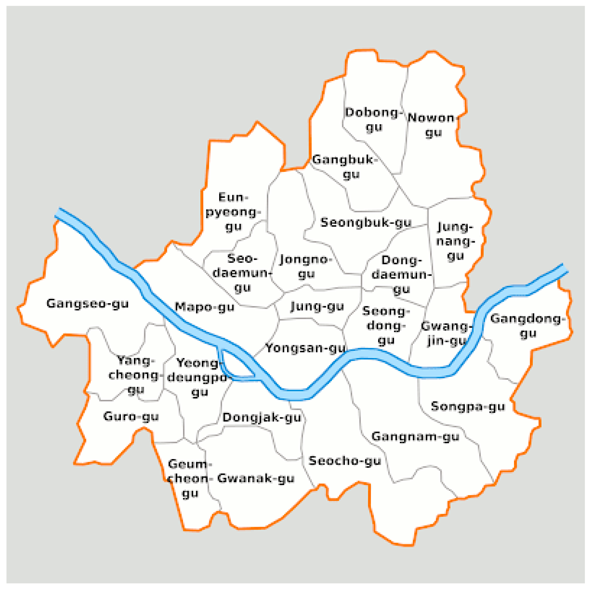
We implemented the model using tensorflow in Python. We used ADAM for the optimizer, early stopping to reduce learning time, and the tensor flow built-in LSTM model. We used a one CPU and GPU workstation to run the experiments. We applied the model to set up, train, and predict the demands of a shared bike operated by Seoul Metropolitan City. There are two types of demand forecasting: district level and station level. We chose five districts (Mapo-gu, Seodaemun-gu, Youngdeungpo-gu, Dongdaemun-gu, and Jongno-gu) out of 25 districts in Seoul Metropolitan City (Figure 2) for the district level, based on the volume of demand and proximity of districts.

Figure 2. Districts of Seoul Metropolitan City.

4.1. Forecasting Demand of Bikes by Districts

We aggregated the daily demand from the rental history of an individual bike since the beginning of the service. We collected Mapo-gu, Seodaemun-gu, and Youngdeungpo-gu data from 19 September 2015 to 30 June 2020 from the beginning of the shared-bike service, while Dongdaemun-gu and Jongno-gu data were collected from 17 July 2016 and 15 October 2015, respectively, because the service in these districts was launched later than in other districts. The data were divided into training and test data. The first 80 percent of the data were labeled as training data, and the later 20 percent were labeled as test data (Table 1).

Table 1. Periods of historical district demand data and the structure of the training dataset.

District	Size of Data	Duration	Size of Training Data	Data Duration for Training Data	Size of Test Data	Data Duration for Test Data
Mapo-Gu	1747	19 September 2015~30 June 2020	1398	19 September 2015~17 July 2019	349	18 July 2019~30 June 2020
Seodaemun-gu	1747	19 September 2015~30 June 2020	1398	19 September 2015~17 July 2019	349	18 July 2019~30 June 2020
Youngdeungpo-gu	1747	19 September 2015~30 June 2020	1398	19 September 2015~17 July 2019	349	18 July 2019~30 June 2020
Dongdaemun-gu	1445	17 July 2016~30 June 2020	1156	17 July 2016~15 September 2019	289	16 September 2019~30 June 2020
Jongno-gu	1721	15 October 2015~30 June 2020	1377	15 October 2015~30 June 2020	344	23 July 2019~30 June 2020

Table 2 describes the demand trend. The daily demand consistently increased in the five districts since the launch of the service. Variability, represented by the coefficient of variations, was between 0.5 and 0.6, which is relatively small. This implies that the social needs for shared bikes are greater than the current service capacity, which consists of the number of bikes, bike redistribution capability, and station capacity. Thus, demand is increasing with small amounts of variability.

Table 2. Data description.

District	Year	Average Daily Demand	Standard Deviation of Daily Demand	Coefficient of Variation
Mapo District	2015	386.20	216.37	0.56
	2016	1116.79	752.20	0.67
	2017	2120.15	1219.07	0.57
	2018	2495.37	1416.22	0.57
	2019	3619.89	1877.56	0.52
	2020	3917.39	1697.18	0.43
	Total	2385.69	1743.11	0.73
Seodaemun District	2015	80.61	45.23	0.56
	2016	291.20	248.95	0.85
	2017	786.50	434.75	0.55
	2018	985.58	514.73	0.52
	2019	1532.93	736.00	0.48
	2020	1630.94	576.72	0.35
	Total	926.23	718.18	0.78
Youngdeungpo District	2015	233.94	153.98	0.66
	2016	812.81	630.53	0.78
	2017	1759.75	1062.63	0.60
	2018	2444.61	1450.77	0.59
	2019	4168.14	2221.80	0.53
	2020	4850.25	2133.83	0.44
	Total	2438.77	2105.08	0.86
Dongdaemun District	2016	420.67	199.25	0.47
	2017	655.95	379.81	0.58
	2018	958.46	524.03	0.57
	2019	1765.50	907.92	0.51
	2020	1949.29	715.69	0.37
	Total	1148.17	834.36	0.73
Jongno District	2015	230.38	120.32	0.52
	2016	673.90	450.27	0.67
	2017	1288.10	703.08	0.55
	2018	1522.28	776.39	0.51
	2019	2090.97	941.70	0.45
	2020	2074.25	780.53	0.38
	Total	14121.62	925.72	0.66

We applied the same model parameters to each district’s model because the properties of the districts’ demand data are identical. The encoder and decoder lengths were 100 and 7, respectively. When the encoder length was shorter than 100, the forecasting errors were significant. The batch size was 16, and the learning rate was $1\times {10}^{-3}$. We used two LSTM layers with 2048 nodes for normal and truncated normal distributions, while 128 nodes were used for negative binomials with two layers.

The running time depends on the assumed distribution. The negative binomial distribution took around 90 s, while the normal and truncated normal distribution both took around 5000 s. The running time is measured from the beginning of training to the end of the distribution evaluation. We found the best hyper-parameters by a grid search. We explored the number of LSTM layers and nodes in addition to the encoder (and decoder) lengths, batch sizes, and learning rates.

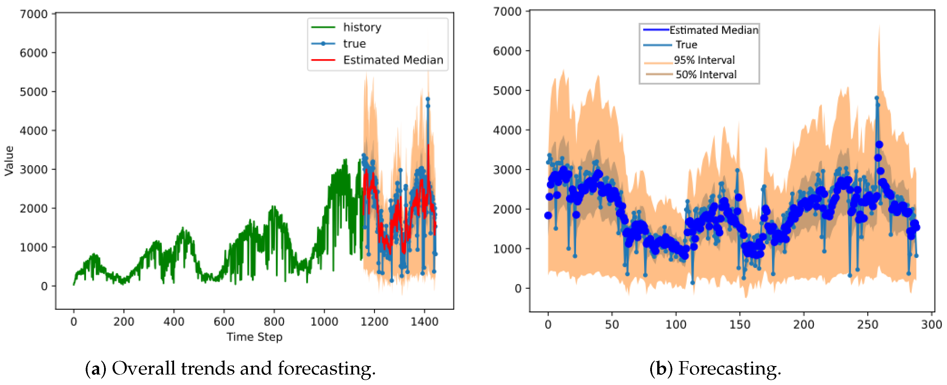
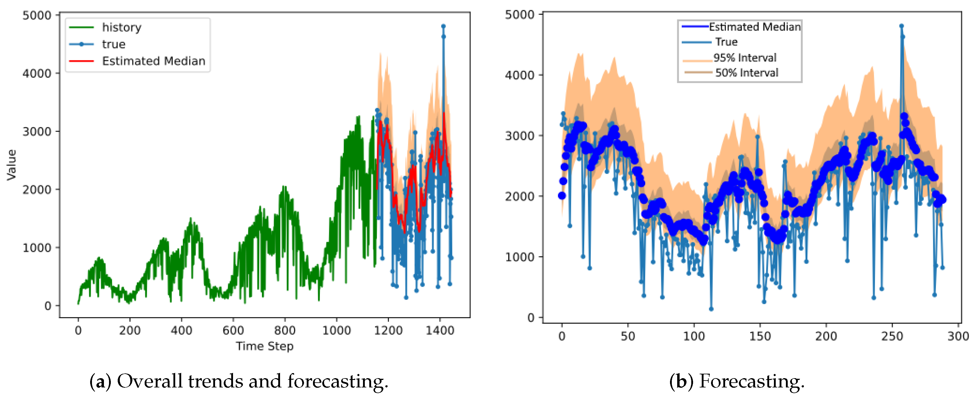
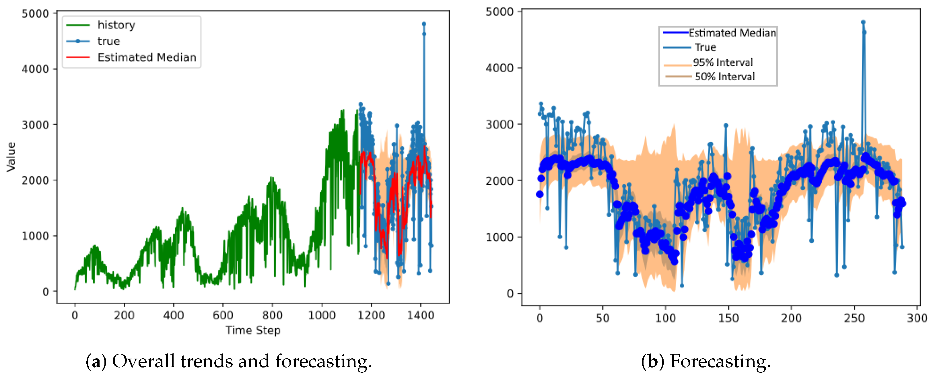
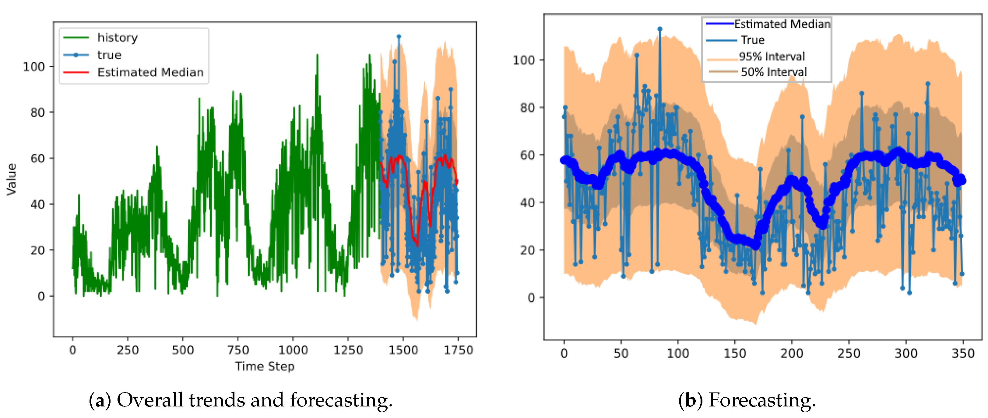
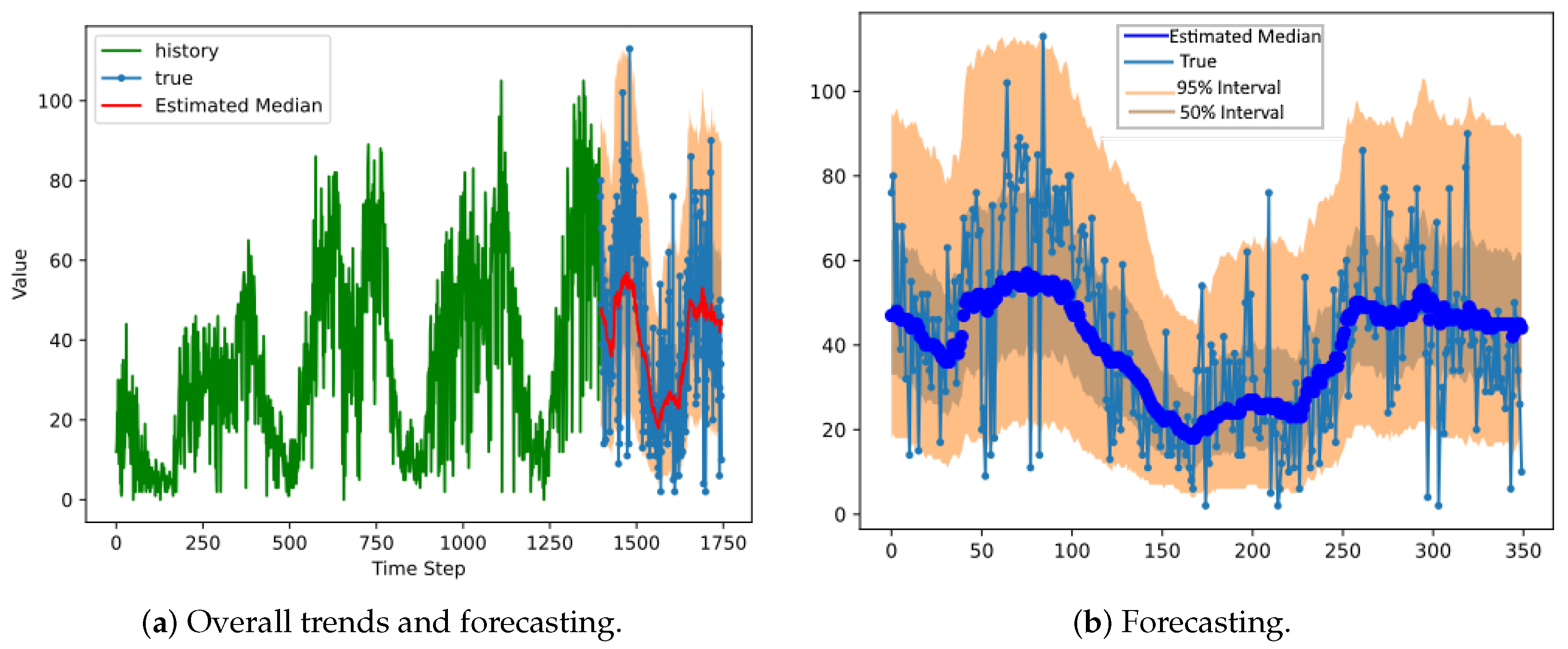
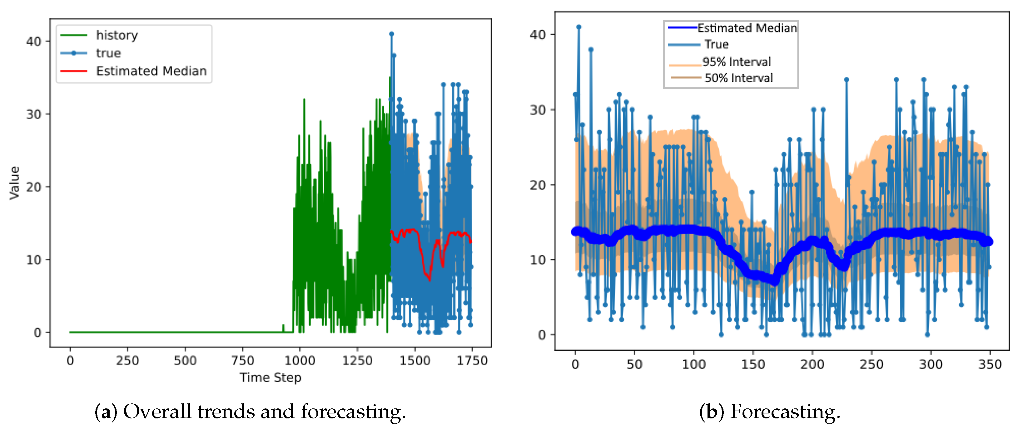
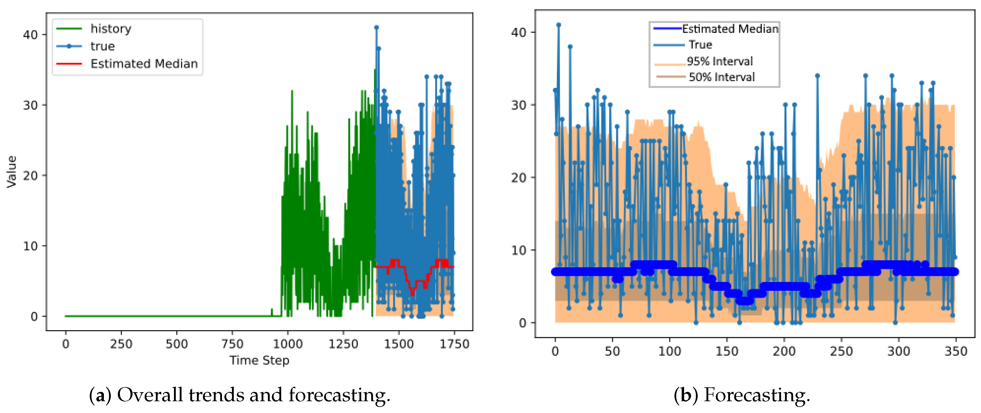
We used Dongdaemun district’s shared-bike rental demand history to forecast the demand. The green and blue lines present the historical demand and real data during the prediction period, respectively. The red line is the estimated median based on the distribution parameters, and the orange area stands for a 95 percent interval (Figure 3, Figure 4 and Figure 5).

Figure 3. The results of DeepAR for a normal distribution in Dongdaemun district.

Figure 4. The results of DeepAR for a truncated normal distribution in Dongdaemun district.

Figure 5. The results of DeepAR for a negative binomial distribution in Dongdaemun district.

According to Dongdaemun district’s forecasting results, the 95 percent interval of normal distribution covers most of the true demand (Figure 3). However, in the truncated normal case (Figure 4), the 95 percent interval lies mostly above the real-data median, which means that it overestimated the demand. The 95 percent negative binomial distribution interval is generally narrower than the normal and truncated normal distributions. The normal distribution resulted in the widest 95 percent interval. The width of the 95 percent interval varies over time in the negative binomial distribution (Figure 3, Figure 4 and Figure 5).

We compared the model accuracy results using negative binomial, normal, and truncated normal distributions (Table 3). Furthermore, we employed statistical models, such as ARIMA, its variants, and the Holt–Winters models, as benchmarks. According to Kim and Lim [26], ARIMAX, which incorporates daily precipitation and temperature as covariates, was the most accurate forecasting method among ARIMA variants. Two accuracy measurement metrics, namely the root mean squared error (RMSE) and the mean absolute percentage error (MAPE) were used (Equations (6) and (7)).

Table 3. Result comparison.

District	Model		RMSE	MAPE
Mapo District	ARIMA (2,1,1)		2088.956	89.477
	ARIMAX (0,1,2)		1378.481	41.167
	Holt–Winters	$\alpha =0,\beta =0,\gamma =0.262$	1911.502	58.631
	DeepAR	Normal Distribution	1305.004	44.894
		Truncated Normal Distribution	1325.812	45.088
		Negative Binomial Distribution	1662.560	47.439
Seodaemun District	ARIMA (4,1,2)		878.415	79.968
	ARIMAX (0,1,2)		996.094	71.095
	Holt–Winters	$\alpha =0.119,\beta =0,\gamma =0.455$	4220.476	233.640
	DeepAR	Normal Distribution	670.769	46.615
		Truncated Normal Distribution	493.624	37.421
		Negative Binomial Distribution	840.847	47.302
Youngdeungpo District	ARIMA (3,1,1)		2477.644	88.779
	ARIMAX (0,1,2)		2308.071	63.687
	Holt–Winters	$\alpha =0,\beta =0,\gamma =0.524$	2008.233	49.97
	DeepAR	Normal Distribution	1769.528	48.224
		Truncated Normal Distribution	1741.432	52.356
		Negative Binomial Distribution	1637.700	46.140
Dongdaemun istrict	ARIMA (2,1,1)		819.346	49.850
	ARIMAX (1,1,1)		908.813	39.241
	Holt–Winters	$\alpha =0.004,\beta =0,\gamma =0.377$	817.888	44.478
	DeepAR	Normal Distribution	558.430	36.257
		Truncated Normal Distribution	595.148	37.254
		Negative Binomial Distribution	700.263	40.867
Jongno District	ARIMA (2,1,2)		966.537	72.600
	ARIMAX (5,1,1)		880.789	39.709
	Holt–Winters	$\alpha =0.048,\beta =0,\gamma =0.477$	1867.731	102.214
	DeepAR	Normal Distribution	755.448	49.873
		Truncated Normal Distribution	785.214	50.882
		Negative Binomial Distribution	1446.910	50.882

The RMSE is for estimating the absolute error, and the MAPE is for the relative error, where $A_t$ is an estimated median computed by the probability distribution at period t, and $F_t$ is the demand observation at period t. In general, DeepAR’s performance was better than ARIMA, its variants, and the Holt–Winters methods for both the RMSE and MAPE. However, while DeepAR outperformed the others, the best assumed distribution for each district varied.

The normal distribution performed best in the Mapo, Dongdaemun, and Jongno districts. The truncated normal distribution was best in Seodaemun District, while it was the second best for other districts. The negative binomial distribution was the most effective in Youngdeungpo District but was outperformed by other distributions in other regions.

$$\mathrm{RMSE}=\sqrt{\frac{{\sum }_{t=1}^T{\left(A_t-F_t\right)}^2}{T}}$$

(6)

$$\mathrm{MAPE}=\frac{1}{T}\sum _{t=1}^T\left|\frac{A_t-F_t}{A_t}\right|$$

(7)

4.2. Forecasting Demand of a Bike Station

We chose five districts in Seoul Metropolitan City and forecast the daily demand of each district. Now, we focused on Mapo District and performed demand forecasting using DeepAR for individual bike stations. While the district-level bike demand is a univariate time series, the demand for all bike stations in a district is a multivariate series that contains a demand time series for all stations.

Users pick up bikes at one station and return them to another, which could maximize the capacity of the latter station. Therefore, it is necessary that a forecasting model effectively reflects the interactions among stations. Salinas et al. [7] showed that the DeepAR model successfully forecasts multiple correlated items. As the DeepAR is based on a deep-learning structure, training the model with multiple time series simultaneously makes it possible to incorporate correlations among bike stations.

There are 73 bike stations in Mapo District. Some of the stations were installed at the launch of the service and, as demand increased, the number of stations gradually increased. Thus, for the stations built after the service launch, there is no demand history for the early time period in the total service period. As our model is built on the encoder–decoder scheme, certain amounts of training data are required to forecast properly. In other words, stations that were set up recently and do not have as extensive demand records were not suitable for training the network. To compare the training performance among stations according to age, we intentionally chose two stations: one that was set up at the service launch, while the other was set up three years later.

Model settings, such as the encoder–decoder lengths, number of LSTM nodes and layers, batch sizes, and learning rates were the same as for forecasting the demand by district. However, the running times were different: 240 s for the negative binomial distribution and 1400 s for the normal and truncated normal distributions.

Figure 6, Figure 7 and Figure 8 show the forecasting results for Station 10. The figures show the median values from the forecast distributions as connected large, solid dots, and the forecasting ranges are displayed as a shaded area. Station 10 was set up at the beginning of the bike-sharing service. A 95 percent interval of normal distribution (shaded area) covers most of the true demand (Figure 3).

Figure 6. The results of DeepAR for a normal distribution at Station 10 in Mapo District.

Figure 7. The results of DeepAR for a truncated normal distribution at Station 10 in Mapo District.

Figure 8. The results of DeepAR for a negative binomial distribution at Station 10 in Mapo District.

However, as in the truncated normal case (Figure 4), the 95 percent interval lies mostly above the median of the real data, which means that it overestimated the demand. If we perform forecasting with the negative binomial distributions (Figure 5), the prediction ranges are somewhat narrower than in normal cases, and thus some actual values are outside the range.

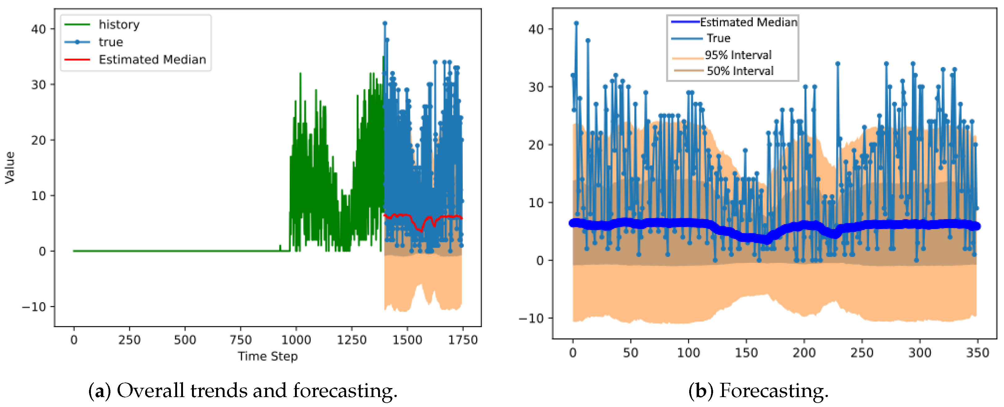
Station 70’s forecasting results are displayed in Figure 9, Figure 10 and Figure 11. Station 70 was established three years after the service launch. Its overall forecasting performance is not as good as Station 10 because of insufficient data. The normal case does not work (Figure 9) because the normal distribution can produce unacceptable negative-valued forecasting. The negative binomial distribution (Figure 11) tends to underestimate the real values. When the truncated normal distribution was used for the distribution model, the estimations of median values followed the fluctuation of actual values accordingly; however, the forecast range did not cover the real-value variability.

Figure 9. The results of DeepAR for a normal distribution at Station 70 in Mapo District.

Figure 10. The results of DeepAR for a truncated normal distribution at Station 70 in Mapo District.

Figure 11. The results of DeepAR for a negative binomial distribution at Station 70 in Mapo District.

Table 4 summarizes the overall prediction performances among the assumed probability distributions. The truncated normal distribution was the best for demand forecasting because of the root mean squared error (RMSE); however, the negative binomial distribution worked best with the mean absolute percentage error (MAPE). Table 4 shows that the MAPE is much larger than the RMSE. We obtained a large MAPE value because the demand for an individual station is too small.

Table 4. Forecasting performance comparison for Mapo District.

Distribution	MAPE	sMAPE	RMSE
Normal	922,302,586.916	3303.598	35.772
Truncated Normal	1,338,800,077.387	3269.955	33.603
Negative Binomial	830,237,199.556	3527.138	37.015

Unlike for the district-level demand, there were days of zero demand, which may make the absolute percentage error impossible to compute (Equation (7)). To prevent computation errors, a small number was added to the zero demand to avoid zero denominators (Equation (8)). This metric is called the symmetric mean absolute percentage error (sMAPE). For a reasonable comparison, the sMAPE was used to measure the performance, and the results are displayed in Table 4.

$$\mathrm{sMAPE}=\frac{1}{T}\sum _{t=1}^T\left|\frac{A_t-F_t}{\frac{F_t+A_t}{2}}\right|$$

(8)

Using the truncated normal distribution was most effective when forecasting the station-level demand with the sMAPE. The truncated normal distribution does not assume negative values unlike the normal. As the station-level demand is relatively smaller compared with the district level and the normal distribution can generate many negative values with the small numbers, the normal is not a realistic choice. That is why the truncated normal distribution performed better than the normal. Consequently, considering sMAPE and RMSE, the truncated normal distribution is recommended for forecasting station-level demand with our model.

We randomly chose four sample stations and measured the predictions, accordingly (as shown in Table 5). In general, the truncated normal distribution performed best when there were zero day demands. If there were no zero daily demands, then the normal distribution showed the best performance. We can easily discover the existence of zero daily demands by checking the MAPE. A large MAPE indicates that there are small denominators. We added a small value to the daily demand to prevent logical errors caused by dividing by zero.

Table 5. Forecasting performance comparison for Station 10 and 70 in Mapo District.

Station	Distribution	MAPE	sMAPE	RMSE
Station 10	Normal	0.763	0.411	26.391
	Truncated Normal	0.666	0.489	32.083
	Negative Binomial	0.676	0.492	31.924
Station 20	Normal	4,193,517,960	0.641	26.453
	Truncated Normal	3,504,414,703	0.560	19.476
	Negative Binomial	3,924,418,606	0.570	19.714
Station 40	Normal	0.567	0.369	17.324
	Truncated Normal	0.563	0.520	23.474
	Negative Binomial	0.551	0.402	18.804
Station 70	Normal	537,598,166	0.817	10.984
	Truncated Normal	579,754,701	0.821	11.206
	Negative Binomial	319,767,443	1.056	12.622

A normal distribution with a large MAPE performed best for Station 70. However, the performance levels between the normal and truncated normal distributions were close. Furthermore, when we compared Figure 9 and Figure 10, we observed that the truncated normal distribution caught the fluctuations of the demand trends; therefore, it is reasonable to argue that the truncated normal distribution performed better than the normal.

5. Conclusions

We implemented DeepAR [7] in our methodology to produce probabilistic forecasting for the bike demand in Seoul’s shared-bike service in Korea. Our work streamlines bike inventory rebalancing and optimal vehicle routing. First, we estimated the future bike demand for each station. Second, we applied a bike inventory control policy to determine the optimal number of bikes to satisfy the intended user demand at every station.

Lastly, we adopted an optimal vehicle-routing strategy to appropriately rebalance the bikes to maximize their use. As the first step, our work provided the demand of bikes as a form of probabilistic distribution, and we used the distribution output in inventory management as the input. We proved that DeepAR is an appropriate methodology that provides a probability distribution as a forecasting output.

Through the computational experiments, we evaluated the performance of the DeepAR model with the bike-sharing dataset at both the district and station levels. We made our forecasting estimates for the evaluation with median values from the probability distributions that we obtained from the model. We compared the model’s performance at the district level compared with benchmark models, such as ARIMA, ARIMAX, and Holt–Winters. As there were too many different station cases, the station-level comparison was not effective. Our results from five adjacent districts with large demand showed that the DeepAR approach outperformed the benchmarks by more than 16 percent and up to 61 percent in error reductions.

The DeepAR model used a recursive neural network with multiple LSTM layers and cells. It simultaneously learned from the demands of all stations and provided their demand distributions because the deep-learning structure learned the correlations of demand among the stations. Large numbers of bike stations exist, and each station’s service-start date differed; therefore, providing and training different forecasting models for each individual station was not a practical and reasonable approach. We demonstrated that, although the forecasting model learned from an aggregated dataset, each individual station’s forecasting was accurate, and these results are compatible with [7].

However, the forecasting power was weaker in stations with smaller dataset ranges, and they were slightly adjusted by the probability distribution selected for training the DeepAR model. Nevertheless, the forecasting estimates (the median values) for the stations with small datasets efficiently followed the fluctuations of actual values with appropriately selected probability distributions.

We trained the DeepAR model to derive the appropriate parameters from predefined probability distributions. That is, we assumed that the observed data were random samples from a certain probability distribution and that the parameters of the distribution varied over time (we used days in our study). We implemented three probability distributions: normal, truncated normal, and negative binomial. Our evaluation results showed that, at the district level, all three distributions were acceptable, although the truncated normal distribution was likely to overestimate the demand. The truncated normal distribution is recommended at the station level because it had the fewest forecasting errors of the three distributions.

In order to improve the forecasting performance, it may be useful to have additional information, such as daily weather conditions, because users are not likely to use bikes when it rains or snows. In addition, this research is limited to daily forecasting estimation from the probability distributions. However, since the designated trucks perform rebalancing work several times a day, demand forecasting for shorter time frames, such as every three hours, is also necessary.

As a future direction of research, we will extend our work to eventually encompass the bike inventory rebalancing problem. Our next steps are, first, to make the forecasting more accurate by accommodating daily weather conditions. Second, we will make short-time-frame demand forecasting. Next, we will investigate optimal inventory management policies based on the probability distributions of demand. Finally, in order to achieve optimal inventory management, we will consider a vehicle-routing problem. In this research, we will determine the optimal routes to satisfy the inventory requirements for each station at each time. Our results on probabilistic forecasting for BSS can also be applied to new personal mobility services. This could be an additional direction for future research.