Can the Carbon Emission Trading Scheme Influence Industrial Green Production in China?

Abstract

Emission trading schemes are effective methods to realize the sustainable development of society by coordinating economic development and environmental protection. While green total factor productivity (GTFP), an effective evaluation index of green production, involves both economic and environmental factors, which corresponds to the political and market-driven nature of ETS. This study investigated whether ETS policy could affect industrial GTFP and how it works. First, based on panel data of 278 cities from 2003 to 2017, this article first introduces industrial GTFP calculated by the SBM-GML model and EBM-GML model separately. Second, this study realizes that the implementation of ETS policy has significant and positive effects on industrial GTFP by establishing a difference-in-differences model. Third, this study reveals that the implementation of ETS policy may increase the industrial GTFP by affecting the amount of industrial labor, industrial added value, CO₂ emission, and industrial wastewater discharge. Fourth, by constructing a TFP index, this study shows that the implementation of ETS policy has no significant impact on the production efficiency of industrial enterprises. Finally, there is regional heterogeneity when studying the effect of ETS policy on industrial GTFP.

1. Introduction

Since the founding of the People’s Republic of China, China’s economy has made remarkable achievements. Especially after the implementation of the reform and opening-up policy in late 1978, China has witnessed remarkable economic development. Industrial (Industry refers to the material production sector engaged in the exploitation of natural resources, and the processing and reprocessing of excavated products and agricultural products [1].) development has always been an indispensable part of China’s economic development: as shown in Figure 1, the share of industrial added value in GDP has steadily increased, from 17.6% in 1952 to more than 30% in recent years, and in some years, the share was even more than 40%.

However, labor and land costs in China have risen sharply; the labor-intensive enterprises that once relied on low technology for China’s development are no longer suitable. In addition, a serious problem caused by the rapid development of industry is the extensive consumption of energy. As shown in Figure 2, in the past two decades, the energy consumption of industrial enterprises accounted for 64% to 73% of the total energy consumption in China. According to data from BP Amoco, China’s energy consumption increased rapidly. After 2009, China has exceeded the United States as the largest energy-consuming country, accounting for more than 24% of global energy consumption in 2019. A large quantity of energy consumption creates serious challenges for the environment. In 2006, China became the world’s largest carbon emission country. From 2007 to 2012, China’s carbon emission increment (CO₂) accounted for 64.8% of the global carbon emission increment [3]. Compared with other countries (the United States, Russia, India and Japan), China’s total CO₂ emissions show an obvious upward trend.

In order to cope with the growth slowdown and the constraints of resources and environment, the industrial structure needs to be optimized. The Chinese government has begun to apply pressure on the green development of enterprises, which means that it has become necessary to focus on the Green Total Factor Productivity (GTFP) of industry. GTFP is an index that involves both economic factors (industrial productivity) and environmental factors (energy consumption and pollutant emission). Thus, when the GTFP is studied, economic and environmental factors should both be taken into account. The emission trading system (ETS) is an effective environmental policy to achieve green and sustainable development [4].

Fortunately, the Chinese government has already realized the importance of trading carbon. In 2011, in order to encourage firms to reduce CO₂ emissions through market mechanisms, the National Development and Reform Commission announced that it would promulgate a pilot on carbon emissions trading, and approved CO₂ ETS pilots in five provinces or municipalities (Beijing, Tianjin, Shanghai, Guangdong, Shenzhen) in 2013 and two provinces (Chongqing, Hubei) in 2014. Currently, the carbon emissions trading scheme has been implemented in eight provinces or municipalities. Beijing, Tianjin, Shanghai, Guangdong, and Shenzhen launched the ETS project in 2013, Chongqing and Hubei started in 2014, and Fujian started in 2017. Furthermore, during the Two Sessions of China in 2021, carbon peaking and carbon neutralization were included in the government work report for the first time. The report says that carbon emissions will reach their peak by 2030 and carbon neutralization will be achieved by 2060. In addition, on 16 July 2021, the national carbon trading market opened in China. This demonstrates the Chinese government’s determination to reduce carbon emissions.

The emission trading mechanism has been considered as an effective way to control emission [5]. However, can CO₂ ETS improve the GTFP of industrial enterprises? There are two views of environmental regulation that have been the focus of academic debate. The first view is that the cost of environmental regulation will have a negative impact on industry, leading to a decline in industrial performance. For instance, Wagner took German manufacturing companies as the research object, and found that environmental regulation will significantly reduce a company’s patent applications [6]. The second view is called the Porter hypothesis, which states that appropriate environmental regulation can encourage enterprises to improve their productivity, offset the cost of environmental protection, and enhance the profitability of enterprises in the market. Lanoie et al. took EU enterprises as the research objects, and found that environmental regulation has a positive effect on technological innovation of enterprises, and under certain conditions, environmental regulation can reduce the cost of enterprises [7].

In previous studies, some scholars focused on the GTFP index [8,9,10,11,12,13], a new indicator for evaluating the green production efficiency of enterprises, which can reflect the carbon emissions of enterprises to a large extent. Some scholars studied ETS policy [14,15,16,17,18,19], an effective strategy for the government to restrict carbon emissions of enterprises and urge them to improve green production. However, there are few scholars focused on both two fields, especially at the city level. Therefore, this study aims to explore how China’s ETS policy can affect the green productivity and inefficiency of industrial enterprises. The purpose and contributions of this research are as follows: firstly, based on panel data of 278 cities, this study estimates industrial GTFP using two different approach, SBM-GML index and EBM-GML index, and explores the impact of ETS on GTFP; secondly, this article explores how different the effects of ETS on GTFP and TFP are and how ETS policy improves the green production efficiency of industrial enterprises; finally, the article examines whether there are regional heterogeneities in the impact of ETS policies on industrial GTFP.

2. Related Literature and Background

2.1. GTFP

In 1957, Robert M. Solow introduced the assumptions of technology neutrality and constant return to scale on the basis of Cobb–Douglas production function. Solow considered the residual value of growth after deducting contribution by labor and capital investment in economic growth as technological progress, which is also known as total factor productivity (TFP) and Solow Residual [20]. TFP includes many factors that cannot be explained by the input of factors, such as technological innovation, organizational innovation, and institutional innovation. Subsequently, more and more economists and mathematicians improved the methodology to measure TFP by using modern mathematical methods such as Malmquist productivity index [21]. After being enriched by some scholars such as Fare et al., the Malmquist productivity index has been widely used in studying TFP [22,23].

There is an obvious weakness of the traditional total factor productivity (TFP) that the TFP ignores a necessary part of production, that is, pollution emission. Thus, some scholars introduced pollution emission together with capital, labor, and energy consumption into production function as inputs [24,25]. However, the output characteristics of pollution emission make it unreasonable to regard it as input. In order to correctly fit the impact of environmental pollution on economic growth, Chambers et al., Chung et al., and Fare et al. successively established the directional distance function (DDF) [26,27,28]; in particular, Chung et al. proposed the Malmquist–Luenberger index calculated by DDF, which includes pollution emission as unexpected output in the total factor productivity accounting framework and estimates green total factor productivity (GTFP) [27]. However, there is a possible problem of infeasible solution when calculating the ML index. As shown in Figure 3, the directional distance function of t year may have no intersection with the frontier of t + 1 year due to rapid technological innovation. In Figure 3, $x_1$, $x_2,$ and $x_3$ represent DMUs (decision making units; in this study, they represent the annual situation in different cities) in the year of t, while $a_1$ and $a_2$ represent DMUs in the year of t + 1. The blue lines represent the frontier of t and t + 1 year, the green lines represent the directional distance function, and the black line represents the global frontier. In order to deal with this problem, Oh proposed a global Malmquist–Luenberger index (GML) [29]. It could overcome the infeasible solution of ML index and satisfy circularity by considering the global frontier. The GML index is a positive number. If the index is greater than 1, it means that the industrial production efficiency in year t + 1 is higher than that in year t. If the index is equal to 1, it means that the industrial production efficiencies in two years are equal. If the index is less than 1, it means that the industrial production efficiency in year t + 1 is lower than that in year t.

In addition, slacks-based measure (SBM) was proposed by Tone, which can avoid the defect that the radial and angular traditional DEA model may overestimate the regional environmental efficiency [30]. The SBM model is used by many scholars [31,32]. However, when unexpected output exists, the relationship between input factors and pollutant emission is “inseparable”, while the relationship between input and output of other factors is separable. The epsilon-based measure (EBM) model is also an advanced method, proposed by Tone and Tsutsui [33]. It is a hybrid model including both radial and non-radial distance functions, but the coefficient of the radial part is not a definite value. In order to make the research more rigorous, this study combines the SBM model with the GML index and the EBM model with the GML index to calculate the relative GTFP.

There are many factors that could influence the GFTP. In previous research, scholars paid more attention to foreign investment [8,9,10], technology innovation [11,12,13,34], trade liberalization [35], environmental regulation [9,36,37,38], finance [39], intellectual property protection [40], labor costs [41], and so on. However, one of the most significant policies, emission trading scheme (ETS), is rarely considered when the GTFP is analyzed.

2.2. ETS

Compared with traditional administrative regulatory measures such as fees and penalties, the market emission reduction mechanism can save transaction costs, promote technological innovation in energy conservation and emission reduction, weaken political resistance and stimulate economic instruments. As a market-oriented instruments, emission trading scheme is an effective method to realize the sustainable development of society by coordinating the contradiction between economic development and environmental protection well [42]. From the previous studies, we learned that the implementation of ETS policy can effectively influence the carbon emissions [14,15,16,17], energy consumption [14,17], renewable energy [18], country’s economy [19], energy efficiency [43], and so on. In addition, Jiang et al. systematically reviewed the research results of China’s carbon emission trading system in three respects: mechanism design, policy and regional connection, and impact evaluation [44]. Based on the analysis of the current situation of China’s carbon trading market, Weng and Xu put forward policy suggestions to optimize the national carbon trading market [45]. Munnings et al. aimed to improve the design and operation of pilot projects based on the performance of carbon exchanges in Guangzhou, Shenzhen, and Shanghai in terms of carbon emissions, so as to provide a reference basis for the construction of a national carbon trading system [46]. Similarly, a significant index which represents the industrial green production, green total factor productivity, is rarely considered when the ETS policy is analyzed.

Difference in differences (DID) is an effective method to analysis the influence of a policy. Chen et al. revealed that the construction of low-carbon cities significantly promotes an increase in the TFP of local enterprises by constructing a DID model [47]. Zhang and Zhang used a DID model to investigate the impact of carbon emissions trading (ETS) policy on low-carbon development in terms of CO₂ emissions, carbon intensity, energy consumption, and energy intensity, they found that there is a positive correlation between carbon trading system and low-carbon transformation, and the impact of ETS policy on low-carbon development will gradually increase over time [17]. Hu et al. noticed that CO₂ ETS decreases CO₂ emission by 15.5% compared to that in nonpilot areas in China by using the DID method [14].

As the above argument shows, almost no study examines the effect of China-ETS policy on GTFP of industrial enterprises. Therefore, in order to show the effect of the ETS policy on the productivity of industrial enterprises, we first estimate GTFP by using two different approaches, SBM-GML index and EBM-GML index, for comparison. Then, we explore how the ETS policy affects GTFP by the difference-in-differences (DID) approach. Third, this paper examines how ETS policy affects GTFP. Finally, this study focuses on whether there is regional heterogeneity in the impact of ETS policies on GTFP.

3. Data

3.1. Constructing GTFP Index

Unclear input or output accounting boundaries or incomplete calculations will directly affect the measurement accuracy of the GTFP, leading to a gap between the research results and the actual results [48]. Based on the reality and the availability of data, referring to previous scholars’ research, we constructed the SBM-GML index and EBM-GML index separately by three inputs (human resource, capital, and energy consumption), one desirable output (output value), and four undesirable outputs (${\mathrm{CO}}_2$ emission, ${\mathrm{SO}}_2$ emission, smoke and dust emission, and wastewater), as shown in

Table 1. Variables for GTFP.

Variables		Explanation
Input	Human resource	Number of industrial laborers in different cities
	Capital	Industrial fixed-assets investment in different cities
	Energy consumption	Industrial electricity consumption in different cities
Output	Output value	Total industrial output value added in different cities
Undesirable value	${\mathrm{CO}}_2$ emission	${\mathrm{CO}}_2$ emission in different cities
	${\mathrm{SO}}_2$ emission	$\mathrm{Industrial} {\mathrm{SO}}_2$ emission in different cities
	Smoke and dust emission	Industrial smoke and dust emission in different cities
	Wastewater	Industrial wastewater discharge in different cities

. In addition, for the data of price variables, this study used real value by deflating.

3.2. Choosing Control Variables

When building the DID model, control variables are significant parts to be studied. Following the previous literature [49,50], this article considers foreign direct investment (FDI), number of patents (P), urban population density population per square kilometer (PD), and GDP per capita (PGDP) as control variables. Because the standard deviations among some variables are too large, this study takes the logarithm of foreign investment, urban population density, and GDP per capita. As for number of patents, because some cities may have no patents in the early part of the year, it adds one first and then takes the logarithm.

3.3. Constructing TFP Index

It is necessary to construct another dependent variable that is not influenced by ETS policy to check the robustness of the model. Thus, we consider TFP as the dependent variable. For TFP, this study constructed the Malmquist index by considering the number of industrial laborers, industrial fixed assets investment, and industrial electricity consumption as input, and industrial value as output.

3.4. Analyzing ETS Policy

Before studying the influence of ETS policy, the pilot areas should be checked first. Based on the availability of the data, the study selected 278 cities as the research objects. Among them, 36 cities are in the ETS policy pilot areas; they belong to Beijing, Tianjin, Shanghai, Hubei, Guangdong, or Chongqing provinces or municipalities. Although Fujian became an ETS policy pilot area in 2017, the data we could obtain are from 2003 to 2017, so the cities in Fujian province were not considered as ETS policy pilot areas. All the data come from the China City Statistical yearbook, Carbon Emission Accounts and Datasets, and the statistical yearbook of each province in China.

Table 2. Statistical analysis.

(a)
	Unit	Mean	SD	Max	Min
Number of industrial laborers	10,000 persons	172,199.1	248,079.2	2,609,248	3100
Industrial fixed assets investment	RMB 10,000	10,222,462.7	13,825,672.5	18,920,5245	165,672
Industrial electricity consumption	10,000 KWh	55,6429.5	905,669.4	1,202,035.1	1016
Industrial added value	RMB 10,000	2,019,621.8	3,677,486.1	52,064,947	575
Industrial output value	RMB 10,000	24,397,937.4	39,033,506.4	324,451,453	0.5
${\mathrm{CO}}_2$ emission	Million tons	25.1	23.0	230.7	1.5
$\mathrm{Industrial} {\mathrm{SO}}_2$ emission	1 ton	62,461.84	83,163.14	152,6334	2
Industrial smoke and dust emission	1 ton	32,506.6	117,934.8	5,168,812	34
Industrial wastewater	10,000 tons	7256.9	9581.1	110,763.0	7
Foreign direct investment	RMB 10,000	491,174.1	1,346,718.3	21,934,572.6	41.4
Number of patents	1 unit	391.33	1764.30	45,970	0
Urban population density	$\mathrm{Population}/ {\mathrm{km}}^2$	430.7	326.4	2661.5	4.7
Per capita GDP	RMB/Person	35,192.6	41,708.5	517,012.8	763.4
(b)
		Pilot Areas		Non Pilot Areas
		Mean	SD	Mean	SD
Industrial employment		367,764.5	502,768.7	143,106.8	162,971.1
Industrial fixed assets investment		14,790,724	23,962,917	9,542,886.7	11,427,903.4
Industrial electricity consumption		1,195,044.9	1,709,595.3	461,428.8	661,647.6
Industrial added value		4,240,094.4	7,154,628.8	1,689,303.5	2,660,507.9
Industrial output value		46,649,618.6	69,147,677.6	21,087,770	30,892,898.8
${\mathrm{CO}}_2$ emission		32.8	40.4	23.9	18.9
$\mathrm{Industrial} {\mathrm{SO}}_2$ emission		60,204.1	111,192.7	62,797.7	78,133.4
Industrial smoke and dust emission		25,437.3	32,564.5	33,558.2	125,743.3
Industrial wastewater		6268.1	8215.4	7404.0	9759.4
Foreign direct investment		1,225,586.8	2,599,022.7	381,922.6	993,183.6
Number of patents		1333.1	4303.8	251.2	817.8
Urban population density		661.9	523.2	396.3	269.3
Per capita GDP		58,382.8	80,968.4	31,742.8	30,516.0

Note: Table 2a shows mean, standard deviation, maximum value, and minimum value of all the data selected. Table 2b divided the data into ETS policy implementation areas and non-policy areas, and this article provides a brief overview of these data. For aesthetic reasons, Table 2a contains descriptions of the units, while Table 2b does not contain descriptions of the units.

shows the statistical analysis of the data.

4. Methods

4.1. Measurement of Green Total Factor Productivity

To calculate the GTFP, this study considered both SBM-GML and EBM-GML methods at the same time.

4.1.1. Models with Undesirable Outputs

SBM Model

In this study, the SBM model was first established according to Tone [18].

Supposing that the number of decision-making units (DMUs) are n, and each of them are recorded as DMU_j (j = 1, 2, …, n). x_i represents input, supposing that there are m inputs, x_i (i = 1, 2, …, m); y_r represents output, supposing that q₁ is the number of outputs, y_r (r = 1, 2, …, q₁); b_s represents undesirable outputs, supposing that q₂ is the number of undesirable outputs, b_s (t = 1, 2, …, q₂). $s_i^{-}$ is the slack variable of input, $s_i^{+}$ is the slack variable of output, and $s_t^{b-}$ is the slack variable of undesirable output. $\lambda$ is the weight vector. In addition, this study mainly considered efficiency under constant returns to scale (CRS). E is efficiency. Based on the above, the SBM model with undesirable output was obtained:

$$E=min \frac{1-\frac{1}{m}{{\displaystyle \sum }}_{i=1}^m\frac{s_i^{-}}{x_{ik}}}{1+\frac{1}{q_1+q_2}({{\displaystyle \sum }}_{r=1}^{q_1}\frac{s_r^{+}}{y_{rk}}+{{\displaystyle \sum }}_{t=1}^{q_2}\frac{s_t^{b-}}{b_{tk}})}$$

(1)

s.t.

$${\displaystyle \sum }_{j=1}^n{x}_{ij}{\lambda }_j+s_i^{-}=x_{ik}, i=1, 2, \dots , m$$

$${\displaystyle \sum }_{j=1}^n{y}_{rj}{\lambda }_j-s_i^{+}=y_{rk}, r=1, 2, \dots ,q_1$$

$${\displaystyle \sum }_{j=1}^n{b}_{tj}{\lambda }_j+s_t^{b-}=b_{tk}, t=1, 2, \dots , q_2$$

$${\lambda }_j, s_i^{-},s_i^{+}, s_t^{b-} \ge 0$$

EBM Model

According to Tone and Tsutsui [21], the basic EBM model is as follows:

$$E=min\theta -{\epsilon }_x{\displaystyle \sum }_{i=1}^m\frac{{\omega }_i^{-}{s}_i^{-}}{x_{ik}}$$

(2)

s.t.

$${\displaystyle \sum }_{j=1}^n{x}_{ij}{\lambda }_j+s_i^{-}=\theta x_{ik}, i=1,\dots , m$$

$${\displaystyle \sum }_{j=1}^n{y}_{rj}{\lambda }_j\ge y_{rk}, r=1,\dots , s$$

$${\lambda }_j, s_i^{-} \ge 0$$

In the model, ${\omega }_i^{-}$ is the weight of input i and satisfies ${\displaystyle \sum }_{j=1}^m{\omega }_i^{-}=1$ (${\omega }_i^{-}\ge 0$). ${\epsilon }_x$ is a key parameter which combines the radial $\theta$ and the non-radial slacks terms.

In this research, since undesirable output needs to be considered, we constructed a new EBM model as Formula (3).

$$E=min\frac{\theta -{\epsilon }_x{{\displaystyle \sum }}_{i=1}^m\frac{{\omega }_i^{-}{s}_i^{-}}{x_{ik}}}{\phi +{\epsilon }_y{{\displaystyle \sum }}_{r=1}^{q_1}\frac{{\omega }_r^{+}{s}_r^{+}}{y_{rk}}+{\epsilon }_b{{\displaystyle \sum }}_{t=1}^{q_2}\frac{{\omega }_t^{b-}{s}_t^{b-}}{b_{tk}}}$$

(3)

s.t.

$${\displaystyle \sum }_{j=1}^n{x}_{ij}{\lambda }_j+s_i^{-}=\theta x_{ik}, i=1, 2, \dots , m$$

$${\displaystyle \sum }_{j=1}^n{y}_{rj}{\lambda }_j-s_i^{+}=\phi y_{rk}, r=1, 2, \dots ,q_1$$

$${\displaystyle \sum }_{j=1}^n{b}_{tj}{\lambda }_j+s_t^{b-}=\phi b_{tk}, t=1, 2, \dots , q_2$$

$${\lambda }_j, s_i^{-},s_i^{+}, s_t^{b-} \ge 0$$

The definitions of the letters are similar to those in previous models.

4.1.2. GML Index

According to Oh [17], the global Malmquist–Luenberger index from t time to t + 1 time can be written as

$$GML\left(x^t,y^t,b^t,x^{t+1},y^{t+1},b^{t+1}\right)=\frac{1+E^G\left(x^t,y^t,b^t\right)}{1+E^G\left(x^{t+1},y^{t+1},b^{t+1}\right)}$$

(4)

where $E^G\left(x^t,y^t,b^t\right)$ represent the distances from DMU to the global frontier, which is calculated from Equations (1) and (3). This paper only focuses on the GML index itself and ignores its further decomposition.

4.1.3. Calculation of GTFP based on the SBM-GML/EBM-GML Model

In addition, this study combined the SBM/EBM model with ML index separately, gaining the advantages of their respective horizontal comparison (i.e., comparison between different DMUs in the same period) and vertical comparison (i.e., comparison between different periods for the same DMU) to compare the relative productivity of all DMUs horizontally and vertically at the same time. First, SBM and EBM models were used to calculate the green development efficiency value of the base period (in this paper, 2008 is the base period). Second, GTFP of different DMUs in each period can be obtained based on the ML index. The GTFP calculation equation of the t-th period of DMU relative to the base period is as follows [21]:

$$GTFP\left(x^t,y^t,b^t\right)=E\left(x^1,y^1,b^1\right)\times GML\left(x^1,y^1,b^1,x^2,y^2,b^2\right)\times \dots \times GML\left(x^t,y^t,b^t, x^{t-1},y^{t-1},b^{t-1}\right)$$

(5)

4.2. Measurement of Total Factor Productivity

According to Caves et al. [8], the Malmquist index can be calculated as follows:

$$M\left(x^{t+1},y^{t+1},x^t,y^t\right)=\sqrt{\frac{D^t\left(x^{t+1},y^{t+1}\right)}{D^t\left(x^t,y^t\right)}\times \frac{D^{t+1}\left(x^{t+1},y^{t+1}\right)}{D^{t+1}\left(x^t,y^t\right)}}$$

(6)

where $D^t\left(x^t,y^t\right)$ and $D^{t+1}\left(x^{t+1},y^{t+1}\right)$ represent the distances from the DMU to its frontier in t period and t+1 period, respectively. $D^t\left(x^{t+1},y^{t+1}\right)$ means distance from the DMU in t + 1 period to the frontier in t period while $D^{t+1}\left(x^t,y^t\right)$ means distance from the DMU in t period to frontier in t + 1 period. Similar to GTFP, this study also considered efficiency under constant returns to scale (CRS). In Equation (7), m represents t and t + 1 while n also represents t and t + 1.

$$D^m\left(x^n,y^n\right)=min\theta$$

(7)

s.t.

$${\displaystyle \sum }_{j=1}^m{y}_j{\lambda }_j\ge \theta y_n$$

$$x_n\ge {\displaystyle \sum }_{j=1}^m{x}_j{\lambda }_j$$

$$\lambda \ge 0$$

4.3. DID Method

To analyze the effect of ETS policy on industrial GTFP, the DID model was established. Because the years of participating in the pilot project are different in different cities, this paper adopted the multi-period double-difference model with different policy implementation times:

$$GFT{P}_{st}=\alpha +\beta D_{st}+\delta X_{st}+A_s+B_t+{\epsilon }_{st}$$

(8)

where $GFT{P}_{st}$ is the dependent variable, which is calculated by the SBM-ML and EBM-ML in s city at t time. $A_s$ and $B_t$ represent individual fixed effect and time fixed effect, respectively, to control the unobservable differences between different individuals and different time points. $X_{st}$ represents a series of control variables: trade volume, foreign investment, investment in industrial pollution control, research and development expenditure, and GDP per capita.${\epsilon }_{st}$ is the error term. The parameter of interest in the model is $\beta$. For each city, the value is 1 if the city is in any of the ETS pilot areas during the year after the implementation of ETS policy; otherwise, $D_{st}$ is equal to 0. For instance, Beijing implemented ETS policy in 2013, while cities in Hubei implemented ETS policy in 2014; thus, in 2013, $D_{st}$ in Beijing is 1, while in Hubei’s cities, it is 0. Coefficient β is an important basis for evaluating the effect of policy implementation, indicating the impact of the emission trading scheme on GTFP.

5. Main Results

5.1. Results of GTFP

Combining the formulas above and the selected data, we could calculate the value of GTFP. According to the evaluation system established, the GML index can be calculated as shown in

Table 3. The average value of GML index.

	Based on SBM Model		Based on EBM Model
	Pilot Areas	Non-Pilot Areas	Pilot Areas	Non-Pilot Areas
2004	0.597839	0.67593	0.592816	0.650692
2005	1.361861	1.296809	1.353838	1.293537
2006	1.583451	1.689337	1.588087	1.56199
2007	1.284531	1.480194	1.268079	1.450308
2008	1.30414	1.0905	1.199184	1.07361
2009	1.878951	1.553328	1.918678	1.65774
2010	1.6034	1.985066	1.795808	2.021819
2011	1.092328	1.131729	1.108117	1.152424
2012	1.112318	1.049001	1.088625	1.056129
2013	2.021067	1.272477	1.833597	1.329562
2014	1.314508	1.580834	1.320042	1.587612
2015	1.576677	1.23058	1.47939	1.125624
2016	1.250382	1.422359	1.168852	1.431732
2017	0.929296	1.732859	0.933664	1.728271

Note: The calculation of the index is based on SBM model and EBM model in 278 cities.

, which shows the average index of GTFP and GML based on SBM and EBM model. In addition, the value of GTFP is shown in Figure 4.

In Table 3, the first and second columns present the average GML index based on SBM model for all the cities in pilot areas and non-pilot areas. The third and fourth columns present the average GML index based on the EBM model for all the cities in pilot areas and non-pilot areas. Comparing the GML indexes in pilot area and non-pilot areas, this study showed that in 2013, the GML indexes in pilot areas were obviously larger than those in non-pilot areas, whether the indexes are based on SBM model or EBM model. This means that in pilot areas, the green total factor productivity in 2013 has changed a lot compared to 2012, while in non-pilot areas, the change in green total factor productivity is not so obvious between 2012 and 2013.

Figure 4 presents the average values of GTFP, which are based on the SBM-GML model and EBM-GML model separately. The variation tendency of GTFP in both pilot areas and non-pilot areas began to change in 2013. In addition, because the pilot areas include some technologically advanced cities, such as Beijing, Shanghai, and Shenzhen, the values of GTFP in pilot areas is higher than those in non-pilot areas. After 2013, the GTFP in pilot areas became larger and the distance of GTFP between pilot areas and non-pilot areas increased. This shows that the implementation of ETS policy will have a positive impact on urban industrial GTFP to a certain extent.

5.2. Relationship between ETS and GTFP

To investigate the specific relationship between the implementation of ETS policy and urban industrial GTFP, this study further established a DID model as in Formula (5) to analyze whether ETS policy can significantly influence industrial GTFP.

In

Table 4. The relationship between ETS and GTFP (based on SBM-GML model).

Variable		(1)	(2)	(3)	(4)	(5)
$D_{st}$		0.3647 *** (0.0465)	0.3538 *** (0.0468)	0.3532 *** (0.0468)	0.3505 *** (0.0468)	0.3484 *** (0.0469)
Annual fixed effect		Y	Y	Y	Y	Y
City fixed effect		Y	Y	Y	Y	Y
Control variables	Log(FDI)	N	−0.0380 ** (0.0179)	−0.0358 ** (0.0179)	−0.0351 * (0.0179)	−0.0362 ** (0.0180)
	Log(P)	N	N	0.0697 ** (0.0338)	0.0701 ** (0.0338)	0.0695 ** (0.0338)
	Log(PD)	N	N	N	0.2252 (0.1380)	0.2184 (0.1383)
	Log(PGDP)	N	N	N	N	0.0572 (0.0700)
Prob > F		0.0000	0.0000	0.0000	0.0000	0.0000
Adj R-squared		0.5040	0.5044	0.5048	0.5051	0.5050

Note: The significance levels of 1%, 5%, and 10% are denoted by ***, **, and *, respectively. Y indicates that the corresponding variable is considered, and N indicates that the corresponding variable is not considered. The values in brackets are standard errors.

, the first column includes the effect of ETS policy on industrial green total factor productivity (calculated by SBM-GML model) with annual fixed effect and city fixed effect. The second column includes the effects of ETS on industrial GTFP with annual fixed effect, city fixed effect, and foreign direct investment as control variables, in order to make the data fluctuation relatively stable, all the control variables adopted logarithms in the calculation. The fifth column includes the effect of ETS on industrial GTFP with annual fixed effect, city fixed effect, and all four control variables.

Table 5. The relationship between ETS and GTFP (based on the EBM-GML model).

Variable		(1)	(2)	(3)	(4)	(5)
$D_{st}$		0.1911 *** (0.0227)	0.1863 *** (0.0228)	0.1858 *** (0.0228)	0.1837 *** (0.0228)	0.1827 *** (0.0228)
Annual fixed effect		Y	Y	Y	Y	Y
City fixed effect		Y	Y	Y	Y	Y
Control variables	Log(FDI)	N	−0.0169 * (0.0087)	−0.0155 * (0.0087)	−0.0149 * (0.0087)	−0.0155 * (0.0088)
	Log(P)	N	N	0.0449 *** (0.0165)	0.0452 *** (0.0165)	0.0449 *** (0.0165)
	Log(PD)	N	N	N	0.1788 *** (0.0672)	0.1755 *** (0.0674)
	Log(PGDP)	N	N	N	N	0.0278 (0.0341)
Prob > F		0.0000	0.0000	0.0000	0.0000	0.0000
Adj R-squared		0.6271	0.6273	0.6280	0.6283	0.6285

Note: The significance levels of 1%, and 10% are denoted by ***, and *, respectively. Y indicates that the corresponding variable is considered, and N indicates that the corresponding variable is not considered. The values in brackets are standard errors.

is similar to Table 4, except that the indexes of GTFP in Table 5 are calculated based on the EBM-ML model.

The results are presented in Table 4 and Table 5, and show the similar relationship between the implementation of ETS policy and industrial GTFP. It is easy to establish that the implementation of ETS policy has a significant and positive effect on industrial GTFP, as shown in Table 4 and Table 5.

When the industrial GFTP is calculated by SBM-GML model, the coefficient $\beta$ is 0.3647 if the control variables are not considered. If all the control variables are considered, the coefficient $\beta$ is 0.3484, which means that the implementation of ETS policy has a similar influence on industrial GTFP under many different conditions. In addition, this study realized that foreign direct investment and number of patents could also influence the industrial GTFP when the GTFP is calculated by SBM-GML model. Obviously, the number of patents can represent innovation capability to a certain extent, as with the increasing number of patents, the green total factor productivity of an enterprise will increase. In addition, as foreign direct investment increases, the industrial GTFP will decrease. Apparently, overseas enterprises invest for profit instead of improving domestic green production efficiency. At an early stage, many hypotheses were proposed, such as the pollution haven hypothesis and ecological dumping, to prove this. Polluting industries will relocate to jurisdictions with less stringent environmental regulations, and countries that desire more investment will choose less strict environmental standards. This could explain why foreign direct investment has a negative impact on industrial GTFP. As for urban population density, the t value in column (4) is 1.632, while the standard t value of 10% significance level is 1.645, which means that the urban population density also has a significant impact on industrial GTFP to a certain extent.

Table 5 presents the results for cases where the industrial GTFP is calculated by the EBM-GML model. Similar to the results in Table 4, all the coefficients $\beta$ are around 0.18 under different conditions. By contrast, apart from foreign direct investment and number of patents, there is another control variable, urban population density, which can significantly and positively influence industrial GTFP. For urban population density in China, the populous cities are often distributed in the eastern coastal areas, and have convenient public transportation, a large proportion of service industry, and a high level of enterprise science and technology, which contribute to the improvement of industrial GTFP.

When the study considered the raw data of all the control variables, the results were similar to those calculated by logarithmic data. However, under this condition, the control variable per capita GDP significantly increases the industrial GTFP as shown in

Table 6. The relationship between ETS and GTFP.

Variable		SBM-GML	EBM-GML
$D_{st}$		0.2610 *** (0.0474)	0.1253 *** (0.0230)
Annual fixed effect		Y	Y
City fixed effect		Y	Y
Control variables	FDI	−0.0000000266 *** (0.00000000925)	−0.0000000126 *** (0.00000000448)
	P	0.000014 * (0.00000745)	0.0000153 *** (0.00000361)
	PD	0.0001434 (0.0001152)	0.0001232 ** (0.0000558)
	PGDP	0.00000388 *** (0.00000046)	0.0000019 *** (0.000000223)
Prob > F		0.0000	0.0000
Adj R-squared		0.5168	0.6407

Note: The significance levels of 1%, 5%, and 10% are denoted by ***, **, and *, respectively. Y indicates that the corresponding variable is considered. The values in brackets are standard errors.

. Per capita GDP can reflect a country’s development level and degree of industry to some extent. According to a summary of the industrialization of leading industrial countries, the industrialization process includes an initial period that is dominated by light textile industries. There is an expansion period dominated by heavy and chemical industries such as steel, machinery, automobile, and durable consumer goods, and a mature period characterized by assembly industries and deep processing. With the advancement of industrialization, the composition of production factors has shifted from labor intensive and capital intensive to technology and knowledge intensive. Industrialization features a mature period, which puts forward new requirements for the development of high-tech industries. Thus, high per capita GDP can improve industrial green total factor productivity to a certain extent.

5.3. Impact Mechanism

Based on previous research, the implementation of ETS policy has a significant influence on industrial GTFP, but how does it work? In this section, the question of how the implementation of ETS policy affects industrial GTFP is analyzed. First, we constructed Formula (9):

$$Y_{st}=\alpha +\beta D_{st}+\delta X_{st}+A_s+B_t+{\epsilon }_{st}$$

(9)

where $Y_{st}$ represents eight variables which are used to build the GTFP model, namely, industrial labor, industrial fixed assets input, industrial electricity consumption, industrial output value, CO₂ emission, industrial SO₂ emission, industrial smoke and dust emission, industrial wastewater discharge.

Then, we considered the eight variables as dependent variables, and analyzed the relationship between ETS and these variables separately.

Table 7. The relationship between ETS and GTFP-related variables.

(a)
Variables	Number of Industrial Laborers	Industrial Fixed Assets Investment	Industrial Electricity Consumption	Industrial Added Value
$D_{st}$	0.1413 *** (0.0113)	−0.0135 (0.0112)	0.0208 (0.0189)	0.0591 *** (0.0226)
Annual fixed effect	Y	Y	Y	Y
City fixed effect	Y	Y	Y	Y
Log(FDI)	−0.0009 (0.0043)	0.0483 *** (0.0043)	0.0122 * (0.0073)	0.0209 ** (0.0087)
Log(P)	0.1122 *** (0.0081)	−0.0163 ** (0.0081)	0.0082 (0.0136)	0.0335 ** (0.0163)
Log(PD)	0.0932 *** (0.0333)	0.0554 * (0.0331)	−0.0143 (0.0558)	0.2899 *** (0.0666)
Log(PGDP)	0.0410 ** (0.0169)	0.2069 *** (0.0168)	−0.0974 *** (0.0282)	0.4829 *** (0.0337)
Prob>F	0.0000	0.0000	0.0000	0.0000
Adj R-squared	0.9365	0.9561	0.9108	0.8920
(b)
Variables	CO2 Emission	Industrial SO2 Emission	Industrial Smoke and Dust Emission	Industrial Wastewater Discharge
$D_{st}$	−0.0567 (0.0041)	0.0324 (0.0357)	−0.0090 (0.0353)	−0.0961 *** (0.0299)
Annual fixed effect	Y	Y	Y	Y
City fixed effect	Y	Y	Y	Y
Log(FDI)	−0.0071 *** (0.0016)	−0.0248 * (0.0137)	−0.0313 ** (0.0136)	−0.0253 ** (0.0115)
Log(P)	−0.0028 (0.0029)	−0.0876 *** (0.0256)	−0.0329 (0.0255)	−0.1222 *** (0.0216)
Log(PD)	0.0015 (0.0120)	−0.0869 (0.1053)	0.0703 (0.1042)	−0.0398 (0.0883)
Log(PGDP)	0.0729 *** (0.0061)	0.0443 (0.0533)	0.0699 (0.0528)	0.0707 (0.0447)
Prob>F	0.0000	0.0000	0.0000	0.0000
Adj R-squared	0.9870	0.5610	0.5075	0.6265

Note: All the dependent variables are calculated by logarithm of the original data. The significance levels of 1%, 5%, and 10% are denoted by ***, **, and *, respectively. Y indicates that the corresponding variable is considered. The values in brackets are standard errors.

shows the regressions of each variable with ETS policy. As shown in Table 7, four variables were significantly influenced by ETS policy, namely, industrial labor, industrial added value, CO₂ emission, and industrial wastewater discharge.

Many previous studies [37,51] have proved that CO₂ emission is significantly and negatively affected by ETS policy. It is obvious that emission trading scheme policy aims to reduce CO₂ emission. As part of the implementation of ETS policy, many enterprises have realized that if they do not reduce CO₂ emission, they have to purchase a CO₂ emission quota to satisfy their large CO₂ emission demand. If these enterprises could reduce their CO₂ emission, not only do they not need to purchase CO₂ emission quotas but also they could sell their unused CO₂ emission quotas to receive the benefit. In addition, the implementation of ETS policy could also significantly increase the number of industrial laborers, improve industrial added value, and decrease industrial wastewater discharge.

Overall, from this perspective, the implementation of ETS policy may improve industrial GTFP mainly by increasing the number of industrial laborers, improving industrial added value, and decreasing CO₂ emission and industrial wastewater discharge.

5.4. Relationship between ETS and TFP

In order to further test the impact of carbon emission trading scheme on the green production of industrial enterprises, we also studied the impact of carbon emission trading policy on total factor productivity of industrial enterprises. Thus, industrial TFP will be considered as the dependent variable in this section. The results of TFP are shown in Figure 5; the variation trends of TFP between pilot areas and non-pilot areas are similar.

Generally, ETS policy will influence the variables that are environment related only, which means that the impact of ETS policy on industrial TFP should not be significant. Once the parameter estimation result of the parameter of interest is significant, the ETS policy can significantly promote or hinder the TFP, and the above research conclusion will be questioned. Thus, this study selected industrial TFP as the dependent variable and reassesses Formula (8). The results are presented in

Table 8. The relationship between ETS and TFP.

Variables		TFP	Variables		TFP
$D_{st}$		−0.0453 (0.0494)	$D_{st}$		−0.0405 (0.0507)
Annual fixed effect		Y	Annual fixed effect		Y
City fixed effect		Y	City fixed effect		Y
Control variables	Log(FDI)	−0.0023 (0.0192)	Control variables	FDI	0.0000000047 (0.00000000998)
	Log(P)	0.0411 (0.0361)		P	−0.0000119 (0.00000803)
	Log(PD)	0.0244 (0.1475)		PD	0.0001381 (0.0001243)
	Log(PGDP)	0.0269 (0.0747)		PGDP	0.000000402 (0.000000497)
Prob > F		0.8099	Prob > F		0.5454
Adj R-squared		0.2079	Adj R-squared		0.2083

Note: Table 8 shows the relationship between industrial TFP and the implementation of ETS policy. Y indicates that the corresponding variable is considered, and N indicates that the corresponding variable is not considered. The values in brackets are standard errors.

. In Table 8, column 1 contains the results considering the logarithm data of control variables, while column 2 contains the results with raw data of control variables.

From Table 8, it is obvious that the coefficients of $D_{st}$ are not significant regardless of whether the control variables use raw data or logarithm data. Not only from the T value but also from the p value (Prob > F are 0.8099 and 0.5454), we can confirm that the influence is not significant. Thus, ETS policy has no significant impact on industrial TFP, which proves the robustness of the above research conclusions.

5.5. Robustness Checks

In order to test that whether the results are convincing, we conducted a series of robustness checks to further increase the scientific integrity of this article.

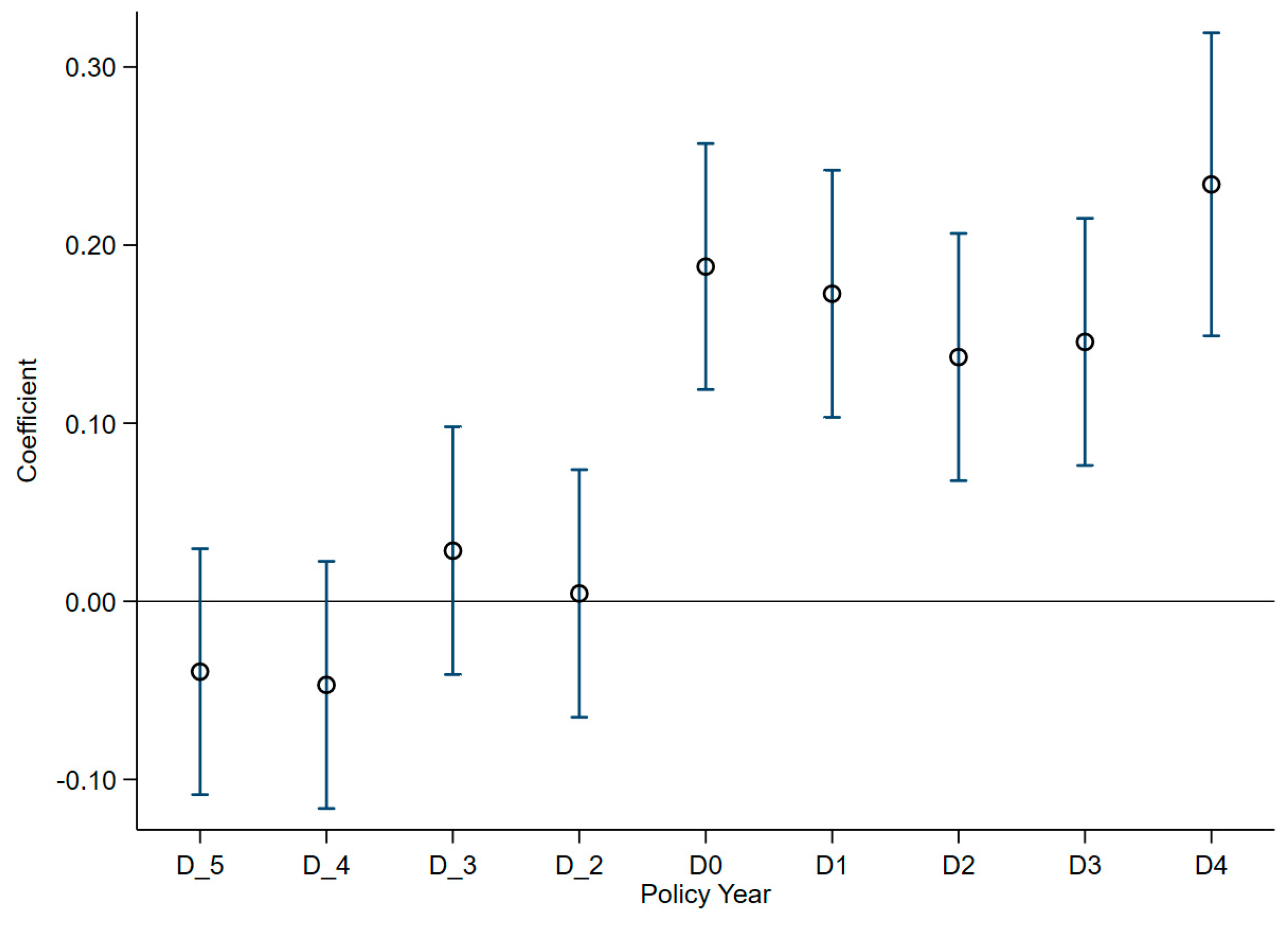
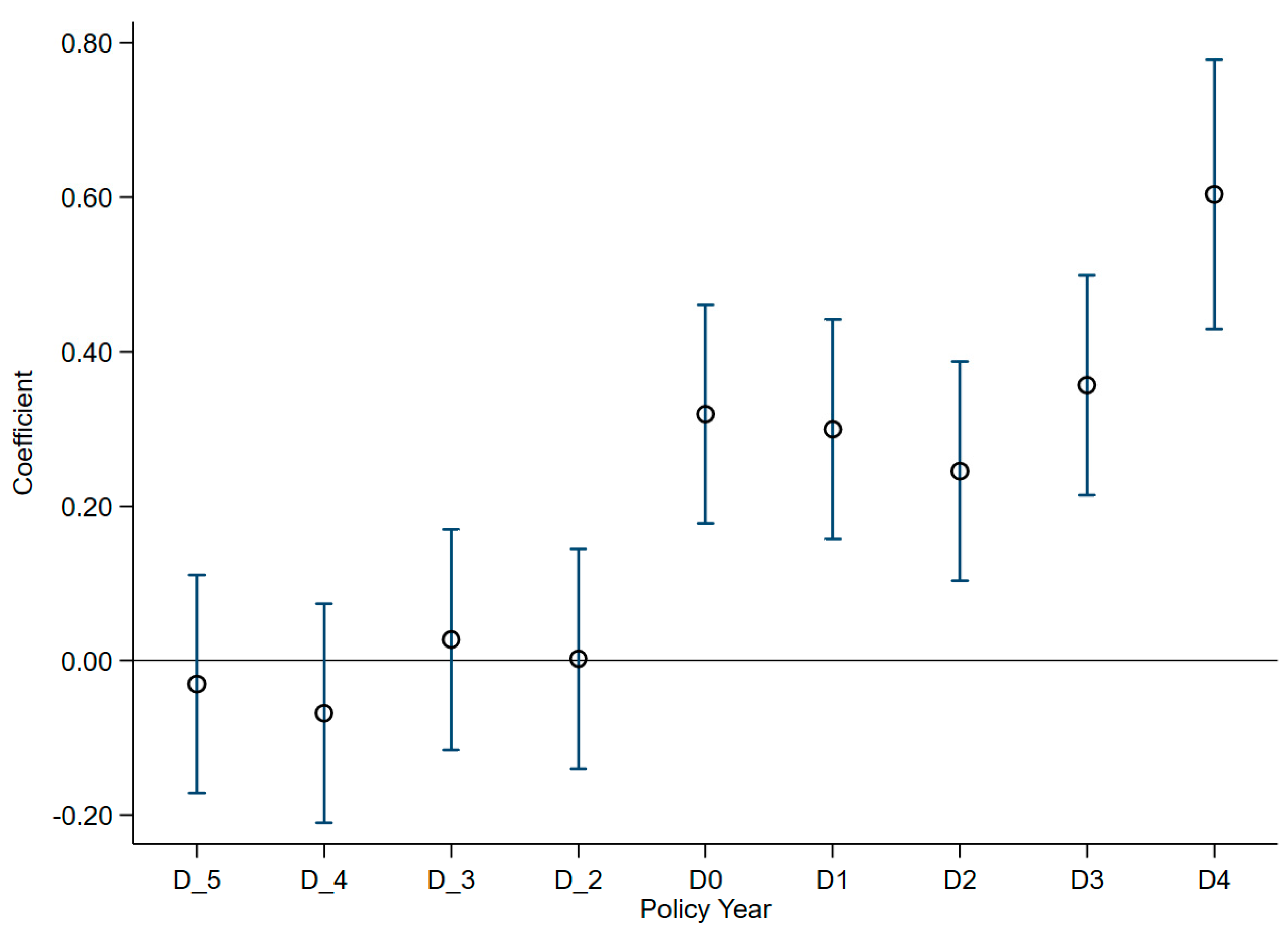
5.5.1. Parallel Trend Test

One of the most important assumptions of the DID model is to satisfy the parallel trend assumption. This refers to the method for parallel trend hypothesis, which was proposed by Beck et al. [52]. Considering a previous study [53], this paper constructed the following two-way fixed effect model to test the parallel trend.

$$GFT{P}_{st}=\alpha +{\beta }_1{D}_{st}^{-5}+{\beta }_2{D}_{st}^{-4}+{\beta }_3{D}_{st}^{-3}+{\beta }_4{D}_{st}^{-2}+{\beta }_5{D}_{st}^0+{\beta }_6{D}_{st}^1+{\beta }_7{D}_{st}^2+{\beta }_8{D}_{st}^3+{\beta }_9{D}_{st}^4+A_s+B_t+{\epsilon }_{st}$$

(10)

In Formula (10), for the provinces or municipalities in the treatment group, if the time is j years after the implementation of the policy, $D_{st}^j$ = 1, otherwise $D_{st}^j$ = 0. In the control group, D is always equal to zero. For instance, Beijing implemented an ETS policy in 2013; for Beijing in 2011, $D_{st}^{-2}$ = 1, and $D_{st}^{-2}$ = 0 in other years in Beijing; for Beijing in 2014, $D_{st}^{+1}$ = 1, and $D_{st}^{+1}$ = 0 in other years in Beijing. While Hubei has implemented an ETS policy in 2014, for a city in Hubei in 2012, $D_{st}^{-2}$ = 1, $D_{st}^{-2}$ = 0 in other years in Hubei. The results are shown in Figure 6 and Figure 7.

In

Table 9. Parallel trend test.

Variables	GTFP
	SBM	EBM
D−5	−0.0306 (0.0861)	−0.0394 (0.0419)
D−4	−0.0680 (0.0864)	−0.0469 (0.0421)
D−3	0.0273 (0.0867)	0.0284 (0.0423)
D−2	0.0025 (0.0866)	0.0044 (0.0422)
D0	0.3194 *** (0.0860)	0.1879 *** (0.0420)
D1	0.2995 *** (0.0864)	0.1727 *** (0.0421)
D2	0.2454 *** (0.0864)	0.1371 *** (0.0422)
D3	0.3568 *** (0.0865)	0.1457 *** (0.0422)
D4	0.6039 *** (0.1060)	0.2341 *** (0.0517)
Annual fixed effect	Y	Y
City fixed effect	Y	Y
Prob>F	0.0000	0.0000
Adj R-squared	0.5049	0.6275

Note: The significance levels of 1% is denoted by ***.

, the first column indicates industrial GTFP value based on the SBM-GML model while the second column is industrial GTFP based on the EBM-GML model. This study reveals that before the implementation of the ETS policy, the trend between the policy pilot cities and non-policy pilot cities are similar.

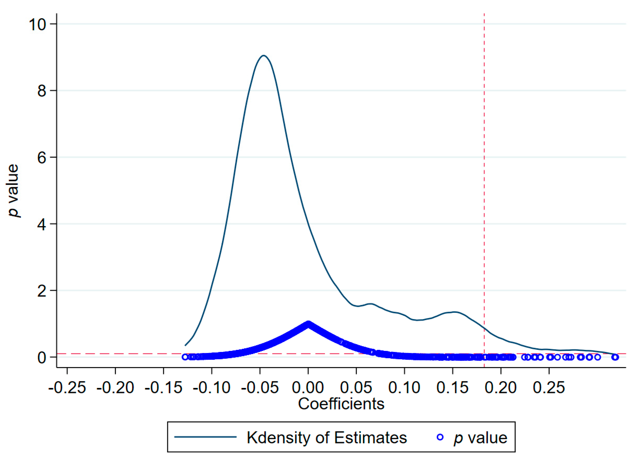
5.5.2. Placebo Test: Randomly Selecting the Treatment Group

In order to further verify that the change in industrial GTFP in the treatment group is really caused by the ETS policy, not by other unobservable factors, the placebo test was performed according to the test protocol of Lu et al. [54]. Thus, 7 provinces were selected from 30 provinces randomly each time to be considered as the treatment groups and the process repeated 1000 times to obtain 1000 estimated coefficients of the model. In addition, 2013 was considered as the base year. Finally, the kernel density map of the estimated coefficients was drawn.

Figure 8 and Figure 9 show the distribution of the estimated coefficients of 1000 hypothetical policy dummy variables and their corresponding p values. Among them, Figure 8 is based on SBM-GML model, while Figure 9 is based on the EBM-GML model. The x-axis represents the size of the estimated coefficients of hypothetical policy dummy variables, the y-axis represents the density value and p value, the curve is the kernel density distribution of the estimated coefficients, the blue dot is the p value corresponding to the estimated coefficients, and the vertical dotted line is the real estimated values of the DID model, which are 0.3484 and 0.1827. Finally, the horizontal dotted line represents a significance level of 0.1.

It can be seen from Figure 8 and Figure 9 that most of the estimated coefficients are concentrated near the zero point, and the coefficient estimation results obtained by quasi-natural experimental design are significantly different from those obtained by placebo test. This indicates that our results are not likely to be obtained by accident, which further proves our conclusion that ETS has a significant positive impact on industrial GTFP.

5.5.3. PSM-DID

To reduce the potential bias of sample selection and overcome the systematic differences in the GTFP trend between a pilot province and non-pilot province, this study considered propensity score matching (PSM) to handle the research samples, and then utilized the DID model to validate the robustness of the initial estimation results.

First, the four control variables were used as matching variables, the ‘kernel’ matching method was used to determine weights, and a ‘logit’ regression was adopted to estimate the results. In this study, due to the limited sample size of the control group, it was suitable to consider 1:1 matching, so we chose ‘neighbor (1)’ specifically to match. Then, ‘common’ was used to exclude the fact that the tendency value in the test group is greater than the maximum tendency value or lower than the minimum tendency value in the control group. It was assumed that the maximum distance allowed between the test group and the matched control is 0.05, so this study selected ‘caliper (0.05)’. In order to give the observation of the test group more than one optimal match at the same time, ‘ties’ was used. After matching, all the samples without match were eliminated regardless of whether they were in the treatment groups or control groups. Finally, we rebuilt the DID method by using the data collected in the last step. The results are presented in

Table 10. PSM-DID results.

Variable		SBM-GML	EBM-GML
$D_{st}$		0.3414 *** (0.0472)	0.1740 *** (0.0230)
Annual fixed effect		Y	Y
City fixed effect		Y	Y
Control variables	Log(FDI)	−0.0366 ** (0.0180)	−0.0160 * (0.0088)
	Log(P)	0.0701 ** (0.0338)	0.0457 *** (0.0166)
	Log(PD)	0.2034 (0.1388)	0.1569 ** (0.0675)
	Log(PGDP)	0.0580 (0.0701)	0.0290 (0.0341)
Prob > F		0.0000	0.0000
Adj R-squared		0.5048	0.6284

Note: Table 10 shows the relationship between industrial GTFP and ETS policy after propensity score matching. The significance levels of 1%, 5%, and 10% are denoted by ***, **, and *, respectively.

. In this table, column 1 contains the results based on the SBM-GML model, while column 2 contains the results based on the EBM-GML model.

According to Table 4, Table 5, Table 10, the coefficients, standard deviations, and t values of $D_{\mathit{st}}$ are almost the same between the results from the DID method and the PSM-DID method. Thus, there is no potential bias of sample selection in this study.

5.6. Heterogeneous Analysis

In order to test whether there is regional heterogeneity in the effect of ETS policy, this article further divided China into three parts according to the division of China National Bureau of Statistics: eastern, central and western regions. The function is as follows:

$$GFT{P}_{st}=\alpha +{\beta }_{1}E{D}_{st}+{\beta }_{2}C{D}_{st}+{\beta }_{3}W{D}_{st}+\delta X_{st}+A_s+B_t+{\epsilon }_{st}$$

(11)

If a city is in the eastern region of China, then E is equal to 1; otherwise, E is equal to 0. Similarly, C is equal to 1 if a city is in the central region of China and C is equal to 1 if a city is in the western region of China.

Table 11. Heterogeneous analysis.

Variables		GTFP
		SBM-GML	EBM-GML
$E{D}_{st}$		0.5058 *** (0.0544)	0.2597 *** (0.0265)
$C{D}_{st}$		−0.0400 (0.0830)	−0.0510 (0.0404)
$W{D}_{st}$		0.1873 (0.2697)	0.2723 ** (0.1313)
Annual fixed effect		Y	Y
City fixed effect		Y	Y
Control variables	Log(FDI)	−0.0306 * (0.0180)	−0.0131 (0.0087)
	Log(P)	0.0715 ** (0.0337)	0.0457 *** (0.0164)
	Log(PD)	0.1783 (0.1379)	0.1540 ** (0.0671)
	Log(PGDP)	0.0755 (0.0699)	0.0369 (0.0340)
Prob > F		0.0000	0.0000
Adj R-squared		0.5088	0.6320

Note: Table 11 shows the relationship between industrial GTFP and the implementation of ETS policy, while the regions of policy areas and non-policy areas have been divided into three parts, eastern, central, and western regions. The significance levels of 1%, 5%, and 10% are denoted by ***, **, and *, respectively.

shows the results of heterogeneous analysis, column 1 contains the results based on the SBM-GML model while column 2 contains the results based on the EBM-GML model. In Table 11, it can be clearly seen that regional heterogeneity does in fact exist. It is obvious that the coefficient of $E{D}_{st}$ is significant and positive, which means in the eastern region, the implementation of ETS policy can effectively influence industrial GTFP. In the western region, the implementation of ETS policy can significantly and positively influence industrial GTFP when the GTFP is calculated by the EBM-GML model. As for the central region, the implementation of ETS policy has no significant effect on industrial GTFP. This sufficiently proves that there is regional heterogeneity in the effect of ETS policy on industrial GTFP.

6. Conclusions

In this article, based on panel data of urban industries, industrial green total factor productivity was first calculated by the SBM-GML model and EBM-GML model, separately. Moreover, this study analyzed the effect of ETS policy on GTFP by establishing the difference-in-differences model. Finally, robustness checks and heterogeneous analysis were employed to ensure the scientific integrity of the results.

Based on the results, the Porter hypothesis is proved to be appropriate to this field in China. As one of the most important environmental regulations, the implementation of a carbon emission trading scheme can significantly improve industrial green total factor productivity. This fully illustrates that ETS policy can not only boost industrial enterprises to protect the environment by conserving energy and reducing emissions but also promote the upgrading and transformation of enterprise production, improve productivity, and bring economic benefits. Moreover, some variables such as foreign direct investment, number of patents, urban population density, and per capita GDP can significantly affect industrial GTFP under different conditions.

In addition, although ETS policy could significantly increase industrial GTFP, the regional heterogeneity does in fact exist. This article reveals that the implementation of ETS policy in the eastern region can significantly improve industrial GTFP. In addition, the implementation of ETS policy in the western region can significantly improve industrial GTFP when the GTFP is calculated by the EBM-GML model. The implementation of ETS policy in the central region has no significant effect on industrial GTFP.

Overall, the implementation of ETS policy can effectively influence industrial GTFP in China, but there are still several issues that need to be resolved in the future, such as how to unify pricing and how to promote it to enterprises and individuals across the whole country.

References

1. National Bureau of Statistics of China. Available online: http://www.stats.gov.cn/tjsj/zbjs/201912/t20191202_1713048.html (accessed on 12 December 2019).
2. National Bureau of Statistics of China. Available online: https://data.stats.gov.cn/english/easyquery.htm?cn=C01 (accessed on 13 December 2021).
3. Jiang, J.; Ye, B.; Xie, D.; Tang, J. Provincial-level carbon emission drivers and emission reduction strategies in China: Combining multi-layer lmdi decomposition with hierarchical clustering. J. Clean. Prod. 2017, 169, 178–190. [Google Scholar] [CrossRef]
4. Naegele, H.; Zaklan, A. Does the eu ets cause carbon leakage in European manufacturing. J. Environ. Econ. Manag. 2019, 93, 125–147. [Google Scholar] [CrossRef]
5. Fang, K.; Zhang, Q.; Song, J.; Yu, C.; Zhang, H.; Liu, H. How can national ETS affect carbon emissions and abatement costs? Evidence from the dual goals proposed by China’s NDCs. Resour. Conserv. Recycl. 2021, 171, 105638. [Google Scholar] [CrossRef]
6. Wagner, M. On the relationship between environmental management, environmental innovation and patenting: Evidence from German manufacturing firms. Res. Policy 2007, 36, 1587–1602. [Google Scholar] [CrossRef]
7. Lanoie, P.; Laurent-Lucchetti, J.; Johnstone, N.; Ambec, S. Environmental policy, innovation and performance: New insights on the porter hypothesis. J. Econ. Manag. Strategy 2011, 20, 803–842. [Google Scholar] [CrossRef]
8. Wang, Z.; Yang, Y.; Wei, Y. Study on Relationship between Environmental Regulation and Green Total Factor Productivity from the Perspective of FDI—Evidence from China. Sustainability 2022, 14, 11116. [Google Scholar] [CrossRef]
9. Qiu, S.; Wang, Z.; Geng, S. How do environmental regulation and foreign investment behavior affect green productivity growth in the industrial sector? An empirical test based on Chinese provincial panel data. J. Environ. Manag. 2021, 287, 112282. [Google Scholar] [CrossRef] [PubMed]
10. Tian, G. How Does Outward Foreign Direct Investment Affect Green Total Factor Productivity? Evidence from Increment and Quality Improvement. Sustainability 2022, 14, 11833. [Google Scholar] [CrossRef]
11. Zhang, D.; Vigne, S.A. How does innovation efficiency contribute to green productivity? A financial constraint perspective. J. Clean. Prod. 2021, 280, 124000. [Google Scholar] [CrossRef]
12. Liu, G.T.; Wang, B.; Chen, Z.X.; Zhang, N. The drivers of China’s regional green productivity, 1999–2013. Resour. Conserv. Recycl. 2020, 153, 104561. [Google Scholar] [CrossRef]
13. Wang, H.; Cui, H.; Zhao, Q. Effect of Green Technology Innovation on Green Total Factor Productivity in China: Evidence from Spatial Durbin Model Analysis. J. Clean. Prod. 2020, 288, 125624. [Google Scholar] [CrossRef]
14. Hu, Y.; Ren, S.; Wang, Y.; Wang, Y.; Chen, X. Can carbon emission trading scheme achieve energy conservation and emission reduction? Evidence from the industrial sector in China. Energy Econ. 2020, 85, 104590. [Google Scholar] [CrossRef]
15. Pietzcker, R.; Osorio, S.; Rodrigues, R. Tightening EU ETS targets in line with the European Green Deal: Impacts on the decarbonization of the EU power sector. Appl. Energy 2021, 293, 116914. [Google Scholar] [CrossRef]
16. Schaefer, S. Decoupling the EU ETS from subsidized renewables and other demand side effects: Lessons from the impact of the EU ETS on CO2 emissions in the German electricity sector. Energy Policy 2019, 133, 110858.1–110858.12. [Google Scholar] [CrossRef]
17. Zhang, Y.; Zhang, J. Estimating the Impacts of Emissions Trading Scheme on Low-Carbon Development. J. Clean. Prod. 2019, 238, 117913. [Google Scholar] [CrossRef]
18. Lin, B.; Jia, Z. Is emission trading scheme an opportunity for renewable energy in China? A perspective of ETS revenue redistributions. Appl. Energy 2020, 263, 114605. [Google Scholar] [CrossRef]
19. Nong, D.; Nguyen, T.H.; Wang, C.; Van Khuc, Q. The environmental and economic impact of the emissions trading scheme (ETS) in Vietnam. Energy Policy 2020, 140, 111362. [Google Scholar] [CrossRef]
20. Solow, R.M. Technical Change and the Aggregate Production Function. Rev. Econ. Stat. 1957, 39, 312–320. [Google Scholar] [CrossRef]
21. Caves, D.W.; Christensen, L.R.; Diewert, W.E. The Economic Theory of Index Numbers and the Measurement of Input, Output and Productivity. Econometrica 1982, 50, 1393–1414. [Google Scholar] [CrossRef]
22. Färe, R.; Grosskopf, S.; Norris, M.; Zhang, Z. Productivity Growth, Technical Progress and Efficiency Change in Industrialized Countries. Am. Econ. Rev. 1994, 84, 66–83. [Google Scholar]
23. Fare, R.; Färe, R.; Fèare, R.; Grosskopf, S.; Lovell, C.K. Production Frontiers; Cambridge University Press: Cambridge, UK, 1994. [Google Scholar]
24. Mohtadi, H. Environment, Growth and Optimal Policy Design. J. Public Econ. 1996, 63, 119–140. [Google Scholar] [CrossRef]
25. Ramanathan, R. An Analysis of Energy Consumption and Carbon Dioxide Emissions in Countries of the Middle East and North Africa. Energy 2005, 30, 2831–2842. [Google Scholar] [CrossRef]
26. Chambers, R.G.; Chung, Y.; Färe, R. Benefit and Distance Function. J. Econ. Theory 1996, 70, 407–419. [Google Scholar] [CrossRef]
27. Chung, Y.; Rolf, F.; Shawna, G. Productivity and Undesirable Outputs: A Directional Distance Function Approach. J. Environ. Manag. 1997, 51, 229–240. [Google Scholar] [CrossRef]
28. Fare, R.; Grosskopf, S.; Pasurka, C.A. Accounting for Air Pollution Emissions in Measures of State Manufacturing Productivity Growth. J. Reg. Sci. 2001, 41, 381–409. [Google Scholar] [CrossRef]
29. Oh, D.H. A global Malmquist-Luenberger productivity index. J. Product. Anal. 2010, 34, 183–197. [Google Scholar] [CrossRef]
30. Tone, K. A slacks-based measure of super-efficiency in data envelopment analysis. Eur. J. Oper. Res. 2002, 143, 32–41. [Google Scholar] [CrossRef]
31. Li, Y.; Chen, Y. Development of an SBM-ML model for the measurement of green total factor productivity: The case of pearl river delta urban agglomeration. Renew. Sustain. Energy Rev. 2021, 145, 111131. [Google Scholar] [CrossRef]
32. Khan, S.U.; Cui, Y.; Khan, A.A.; Ali, M.A.S.; Khan, A.; Xia, X.; Liu, G.; Zhao, M. Tracking sustainable development efficiency with human-environmental system relationship: An application of DPSIR and super efficiency SBM model. Sci. Total Environ. 2021, 783, 146959. [Google Scholar] [CrossRef] [PubMed]
33. Tone, K.; Tsutsui, M. An epsilon-based measure of efficiency in DEA-A third pole of technical efficiency. Eur. J. Oper. Res. 2010, 207, 1554–1563. [Google Scholar] [CrossRef]
34. Liu, Y.; Feng, C. What drives the fluctuations of “green” productivity in China’s agricultural sector? A weighted Russell directional distance approach. Resour. Conserv. Recycl. 2019, 147, 201–213. [Google Scholar] [CrossRef]
35. Jiang, Y.; Wang, H.; Liu, Z. The impact of the free trade zone on green total factor productivity—Evidence from the shanghai pilot free trade zone. Energy Policy 2021, 148, 112000. [Google Scholar] [CrossRef]
36. Fang, Y.; Cao, H. Environmental Decentralization, Heterogeneous Environmental Regulation, and Green Total Factor Productivity—Evidence from China. Sustainability 2022, 14, 11245. [Google Scholar] [CrossRef]
37. Zhang, B.B.; Yu, L.; Sun, C.W. How does urban environmental legislation guide the green transition of enterprises? Based on the perspective of enterprises’ green total factor productivity. Energy Econ. 2022, 110, 106032. [Google Scholar] [CrossRef]
38. Zhuo, C.F.; Xie, Y.P.; Mao, Y.H.; Chen, P.Q.; Li, Y.Q. Can cross-regional environmental protection promote urban green development: Zero-sum game or win-win choice? Energy Econ. 2021, 106, 105803. [Google Scholar] [CrossRef]
39. Lee, C.C.; Lee, C.C. How does green finance affect green total factor productivity? Evidence from China. Energy Econ. 2022, 107, 105863. [Google Scholar] [CrossRef]
40. Mao, K.; Failler, P. Does Stronger Protection of Intellectual Property Improve Sustainable Development? Evidence from City Data in China. Sustainability 2022, 14, 14369. [Google Scholar] [CrossRef]
41. Qian, W.; Wang, Y. How Do Rising Labor Costs Affect Green Total Factor Productivity? Based on the Industrial Intelligence Perspective. Sustainability 2022, 14, 13653. [Google Scholar] [CrossRef]
42. Wang, H.; Chen, Z.; Wu, X.; Nie, X. Can a Carbon Trading System Promote the Transformation of a Low-Carbon Economy Under the Framework of the Porter Hypothesis?—Empirical Analysis Based on the PSM-DID Method. Energy Policy 2019, 129, 930–938. [Google Scholar] [CrossRef]
43. Hong, Q.D.; Cui, L.H.; Hong, P.H. The impact of carbon emissions trading on energy efficiency: Evidence from quasi-experiment in China’s carbon emissions trading pilot. Energy Econ. 2022, 110, 106025. [Google Scholar] [CrossRef]
44. Jiang, J.; Xie, D.; Ye, B.; Shen, B.; Chen, Z. Research on China’s cap-and-trade carbon emission trading scheme: Overview and outlook. Appl. Energy 2016, 178, 902–917. [Google Scholar] [CrossRef]
45. Weng, Q.; Xu, H. A Review of China’s Carbon Trading Market. Renew. Sustain. Energy Rev. 2018, 91, 613–619. [Google Scholar] [CrossRef]
46. Munnings, C.; Morgenstern, R.D.; Wang, Z.; Liu, X. Assessing the Design of Three Carbon Trading Pilot Programs in China. Energy Policy 2016, 96, 688–699. [Google Scholar] [CrossRef]
47. Chen, H.; Guo, W.; Feng, X.; Wei, W.D.; Liu, H.B.; Feng, Y.; Gong, W.Y. The impact of low-carbon city pilot policy on the total factor productivity of listed enterprises in China. Resour. Conserv. Recycl. 2021, 169, 105457. [Google Scholar] [CrossRef]
48. Fang, C.; Cheng, J.; Zhu, Y.; Chen, J.; Peng, X. Green Total Factor Productivity of Extractive Industries in China: An explanation from Technology Heterogeneity. Resour. Policy 2020, 70, 101933. [Google Scholar] [CrossRef]
49. Li, C.; Qi, Y.; Liu, S.; Wang, X. Do carbon ETS pilots improve cities’ green total factor productivity? Evidence from a quasi-natural experiment in China. Energy Econ. 2022, 108, 105931. [Google Scholar] [CrossRef]
50. Zhang, S.; Wang, Y.; Hao, Y.; Liu, Z. Shooting two hawks with one arrow: Could China’s emission trading scheme promote green development efficiency and regional carbon equality? Energy Econ. 2021, 101, 105412. [Google Scholar] [CrossRef]
51. Gao, Y.; Li, M.; Xue, J.; Liu, Y. Evaluation of effectiveness of China’s carbon emissions trading scheme in carbon mitigation. Energy Econ. 2020, 90, 104872. [Google Scholar] [CrossRef]
52. Beck, T.; Levine, R.; Levkov, A. Big Bad Banks? The Winners and Losers from Bank Deregulation in the United States. J. Financ. 2010, 65, 1637–1667. [Google Scholar] [CrossRef]
53. Gu, Y.; Jiang, C.; Zhang, J.; Zou, B. Subways and Road Congestion. Am. Econ. J. Appl. Econ. 2021, 13, 83–115. [Google Scholar] [CrossRef]
54. Lu, Y.; Tao, Z.; Zhu, L. Identifying FDI spillovers. J. Int. Econ. 2017, 107, 75–90. [Google Scholar] [CrossRef]
Figure 1. Proportion of industrial added value in GDP. Data source: National Bureau of Statistics of China [2].
Sustainability 14 15829 g001
Figure 2. Proportion of industrial energy use in total energy use. Data source: National Bureau of Statistics of China [2].
Sustainability 14 15829 g002
Figure 3. Global directional distance function and frontier.
Sustainability 14 15829 g003
Figure 4. Average value of GTFP from 2003 to 2017.
Sustainability 14 15829 g004
Figure 5. The average value of TFP from 2003 to 2017.
Sustainability 14 15829 g005
Figure 6. Parallel trend test based on SBM-GML model.
Sustainability 14 15829 g006
Figure 7. Parallel trend test based on the EBM-GML model.
Sustainability 14 15829 g007
Figure 8. Placebo test based on SBM-GML model.
Sustainability 14 15829 g008
Figure 9. Placebo test based on the EBM-GML model.
Sustainability 14 15829 g009