

Research on Urban Distribution Routes Considering the Impact of Vehicle Speed on Carbon Emissions

Abstract
:1. Introduction
2. Description of the Problem and Setting of Relevant Variable
- S1: The number of vehicles in the distribution center is limited but meets the distribution needs.
- S2: The storage capacity of the distribution center can meet the needs of all customers.
- S3: The demand of each customer is fixed.
- S4: Normal traffic congestion is considered without any unexpected accidents.
- S5: The speed of the vehicle is time varying.
- S6: The distribution vehicle must return to the distribution center after completing the distribution from the starting point.
- S7: The demand of each customer is less than the prescribed carrying weight of the vehicle.
- S8: Each customer must be served in the specified time window.
- S9: Each customer can only be served by one vehicle and can only be served once.
- S10: In the process of distribution, the vehicle can pass through at most two types of roads to complete the distribution requirements.
2.1. Setting of Relevant Variables
2.1.1. The Change of Vehicle Speed under Multiple Road Types in Different Time Periods
2.1.2. Calculating the Delivery Time under Varying Vehicle Speed
2.1.3. Calculating Carbon Emissions Considering Vehicle Speed
2.2. The Proposed Model Considering the Impact of Varying Speeds on Carbon Emissions
2.2.1. Symbol Definition
- : Set of customers’ nodes,;
- : Set of vehicles, ;
- : Set of paths between customers;
- : Subset of customer nodes, where , is the number of customers in the SC;
- : Demand of customer;
- : Capacity of vehicle ;
- : Distribution center is open from 0 and closed at T;
- : The earliest and latest time range expected by the customer;
- : The time range within which delivery can be accepted beyond the customer’s desired time window, and ;
- : The stay time of the delivery vehicle at customer ;
- : Distance between customers and ;
- : The cost of service quality;
- : Travel time between customers and ;
- : The time that vehicle k returns to the distributor center;
- : The carbon emissions from vehicle k on path ;
- : The total number of distribution points;
- : Satisfaction at distribution ;
- : The total carbon emissions during the distribution;
- : Penalty cost at the distribution point .
2.2.2. Formula
- Minimizing the number of delivery vehicles
- 2.
- Maximize customer satisfaction
- 3.
- Minimizing carbon emissions
2.3. Solution Approach
- The chromosomal code
- 2.
- Generation of the initial population
- 3.
- Fitness calculation
- 4.
- Selection operation
- 5.
- Cross operation
- 6.
- Mutation operation
- 7.
- Evolution reversal operation
- 8.
- Algorithm termination
3. Experimental Results
3.1. Experimental Background and Parameter Setting
3.2. Simulation Results and Analysis
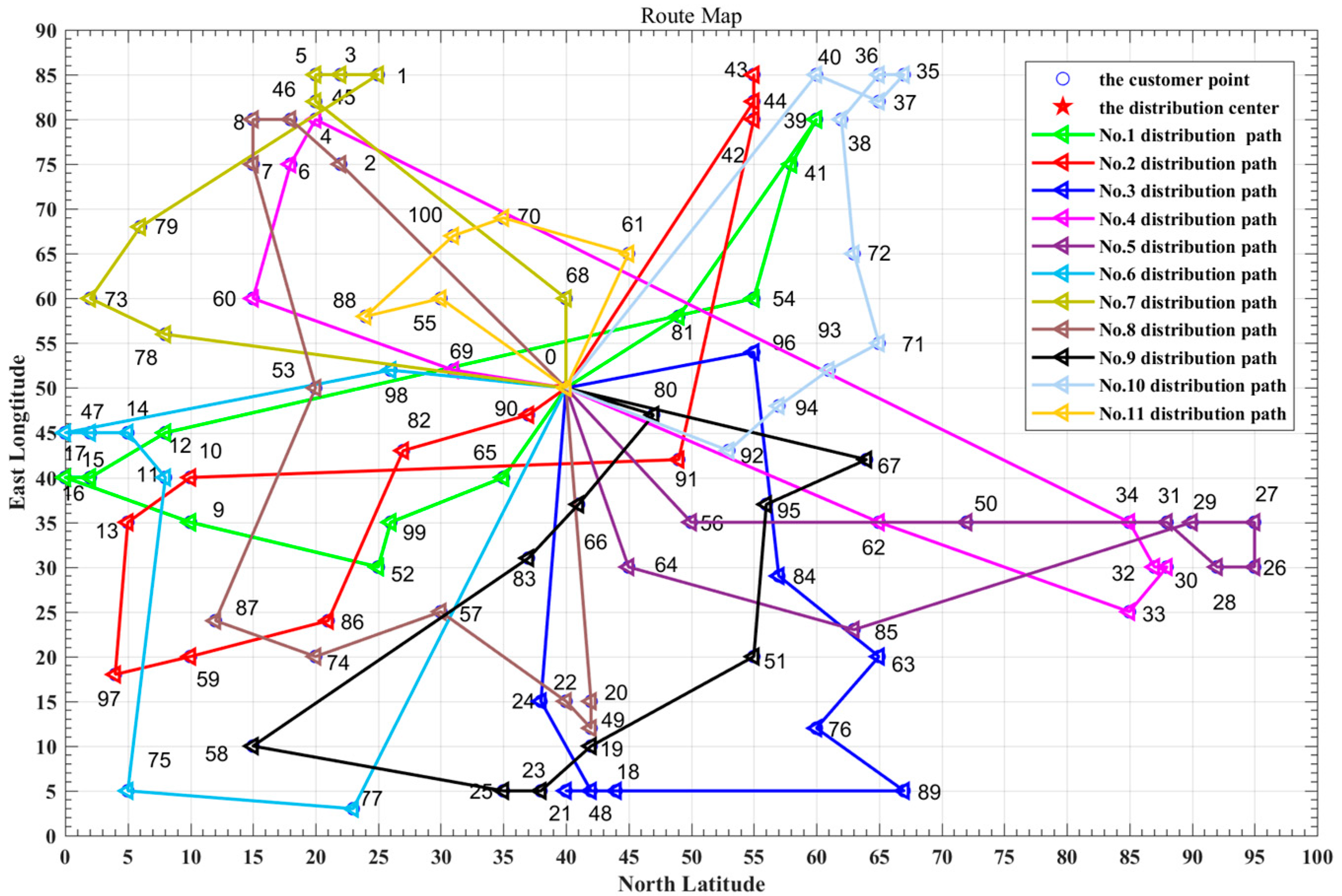
3.2.1. Distribution Path under a Static Road Network
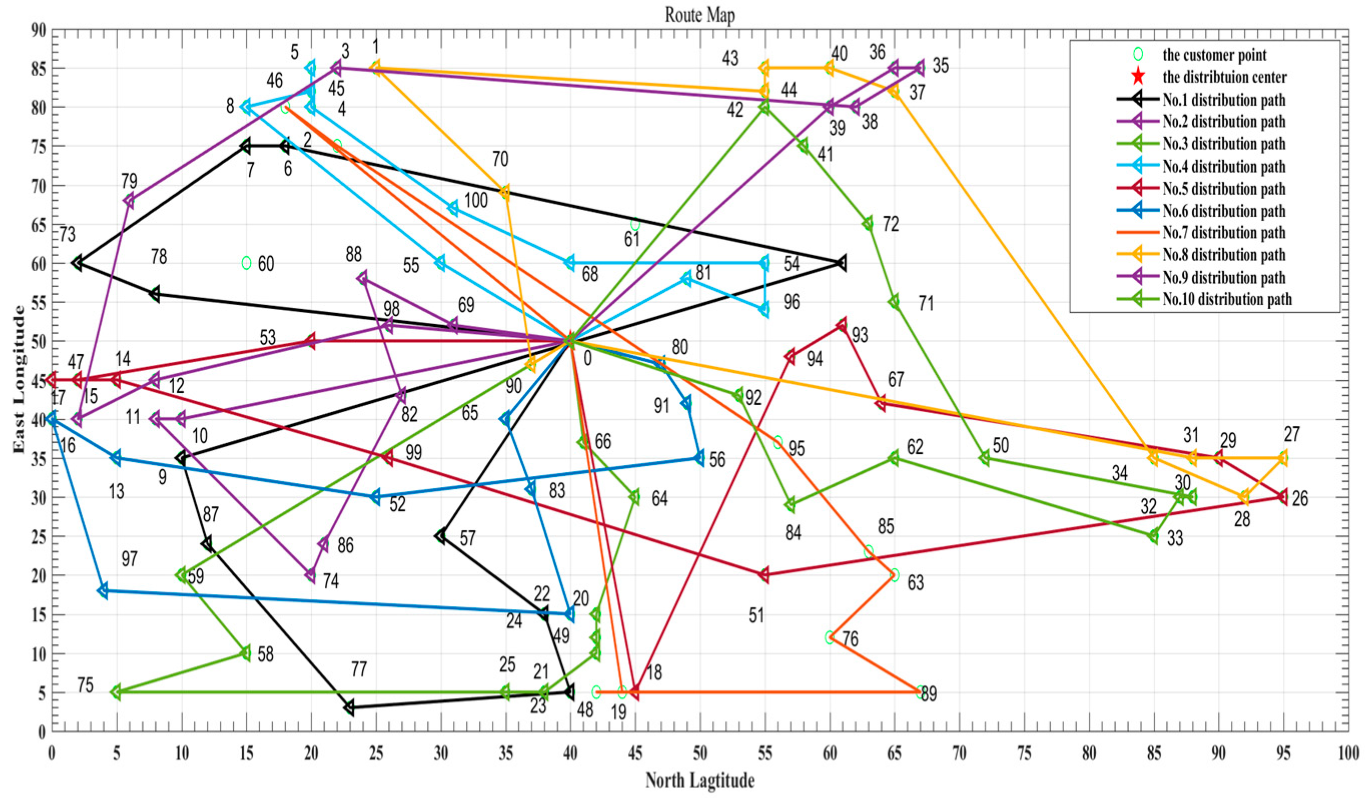
3.2.2. Distribution Path under a Dynamic Road Network
3.2.3. Comparison and Analysis
- 1.
- Optimization comparison between a static road network and a dynamic road network
- 2.
- Optimization comparison of different algorithms
4. Conclusions
Author Contributions
Funding
Institutional Review Board Statement
Informed Consent Statement
Data Availability Statement
Conflicts of Interest
Appendix A

| Start Time | End Time | Main Road | Secondary Road | Express Road | Branch Road |
|---|---|---|---|---|---|
| 0:00:00 | 0:20:00 | 54.077 | 41.416 | 52.061 | 36.559 |
| 0:20:00 | 0:40:00 | 53.366 | 44.291 | 50.596 | 38.132 |
| 0:40:00 | 1:00:00 | 54.568 | 44.294 | 48.392 | 38.285 |
| 1:00:00 | 1:20:00 | 55.345 | 43.912 | 55.668 | 36.186 |
| 1:20:00 | 1:40:00 | 56.565 | 43.511 | 54.619 | 37.465 |
| 1:40:00 | 2:00:00 | 58.817 | 46.157 | 55.174 | 36.436 |
| 2:00:00 | 2:20:00 | 57.406 | 46.481 | 55.925 | 37.376 |
| 2:20:00 | 2:40:00 | 57.897 | 48.084 | 55.884 | 38.253 |
| 2:40:00 | 3:00:00 | 57.672 | 47.193 | 54.570 | 38.558 |
| 3:00:00 | 3:20:00 | 57.886 | 48.175 | 55.114 | 38.274 |
| 3:20:00 | 3:40:00 | 56.306 | 47.355 | 57.024 | 39.746 |
| 3:40:00 | 4:00:00 | 58.668 | 47.038 | 51.820 | 39.071 |
| 4:00:00 | 4:20:00 | 56.815 | 46.910 | 57.726 | 38.828 |
| 4:20:00 | 4:40:00 | 56.467 | 44.484 | 54.405 | 38.357 |
| 4:40:00 | 5:00:00 | 58.079 | 47.318 | 53.294 | 40.304 |
| 5:00:00 | 5:20:00 | 57.397 | 47.049 | 54.439 | 40.396 |
| 5:20:00 | 5:40:00 | 55.832 | 45.153 | 55.270 | 37.757 |
| 5:40:00 | 6:00:00 | 58.489 | 45.054 | 56.157 | 37.673 |
| 6:00:00 | 6:20:00 | 58.425 | 45.050 | 58.548 | 36.092 |
| 6:20:00 | 6:40:00 | 57.905 | 44.094 | 55.500 | 38.872 |
| 6:40:00 | 7:00:00 | 56.471 | 42.368 | 53.773 | 39.965 |
| 7:00:00 | 7:20:00 | 55.759 | 40.332 | 52.385 | 39.522 |
| 7:20:00 | 7:40:00 | 51.893 | 39.501 | 49.071 | 37.915 |
| 7:40:00 | 8:00:00 | 42.891 | 38.622 | 48.634 | 35.851 |
| 8:00:00 | 8:20:00 | 34.953 | 40.290 | 44.671 | 30.090 |
| 8:20:00 | 8:40:00 | 36.392 | 39.951 | 45.372 | 29.845 |
| 8:40:00 | 9:00:00 | 40.562 | 38.233 | 45.340 | 26.517 |
| 9:00:00 | 9:20:00 | 32.487 | 37.594 | 44.454 | 25.094 |
| 9:20:00 | 9:40:00 | 27.775 | 36.722 | 41.236 | 29.977 |
| 9:40:00 | 10:00:00 | 27.906 | 35.560 | 41.539 | 31.797 |
| 10:00:00 | 10:20:00 | 28.851 | 33.377 | 42.539 | 31.522 |
| 10:20:00 | 10:40:00 | 39.624 | 35.739 | 45.421 | 32.608 |
| 10:40:00 | 11:00:00 | 35.281 | 35.742 | 38.205 | 32.966 |
| 11:00:00 | 11:20:00 | 39.546 | 36.170 | 43.475 | 31.999 |
| 11:20:00 | 11:40:00 | 50.661 | 36.798 | 46.391 | 24.992 |
| 11:40:00 | 12:00:00 | 51.140 | 35.992 | 45.928 | 30.904 |
| 12:00:00 | 12:20:00 | 50.646 | 30.776 | 50.108 | 33.768 |
| 12:20:00 | 12:40:00 | 52.140 | 25.366 | 45.928 | 33.004 |
| 12:40:00 | 13:00:00 | 52.243 | 22.081 | 49.100 | 34.512 |
| 13:00:00 | 13:20:00 | 52.005 | 21.422 | 46.849 | 36.584 |
| 13:20:00 | 13:40:00 | 51.870 | 37.446 | 45.978 | 35.983 |
| 13:40:00 | 14:00:00 | 49.470 | 36.338 | 45.539 | 34.593 |
| 14:00:00 | 14:20:00 | 46.877 | 36.852 | 43.231 | 33.558 |
| 14:20:00 | 14:40:00 | 46.544 | 37.435 | 43.862 | 33.290 |
| 14:40:00 | 15:00:00 | 47.215 | 35.062 | 43.373 | 30.797 |
| 15:00:00 | 15:20:00 | 45.602 | 33.433 | 44.624 | 24.425 |
| 15:20:00 | 15:40:00 | 48.717 | 28.954 | 36.542 | 17.717 |
| 15:40:00 | 16:00:00 | 49.864 | 26.772 | 33.017 | 20.156 |
| 16:00:00 | 16:20:00 | 48.936 | 23.609 | 16.796 | 33.754 |
| 16:20:00 | 16:40:00 | 48.611 | 21.906 | 16.952 | 34.152 |
| 16:40:00 | 17:00:00 | 45.517 | 19.608 | 18.931 | 33.186 |
| 17:00:00 | 17:20:00 | 43.247 | 16.398 | 37.891 | 30.653 |
| 17:20:00 | 17:40:00 | 45.876 | 16.453 | 24.006 | 28.573 |
| 17:40:00 | 18:00:00 | 47.757 | 14.741 | 10.090 | 21.654 |
| 18:00:00 | 18:20:00 | 38.553 | 16.895 | 10.887 | 19.401 |
| 18:20:00 | 18:40:00 | 34.615 | 15.621 | 11.054 | 16.898 |
| 18:40:00 | 19:00:00 | 44.695 | 14.154 | 8.513 | 16.552 |
| 19:00:00 | 19:20:00 | 53.397 | 18.317 | 8.329 | 19.455 |
| 19:20:00 | 19:40:00 | 52.343 | 16.244 | 9.292 | 29.737 |
| 19:40:00 | 20:00:00 | 49.304 | 14.614 | 8.766 | 33.422 |
| 20:00:00 | 20:20:00 | 47.298 | 13.551 | 10.377 | 35.110 |
| 20:20:00 | 20:40:00 | 51.715 | 16.009 | 12.783 | 36.117 |
| 20:40:00 | 21:00:00 | 51.439 | 21.017 | 23.870 | 34.724 |
| 21:00:00 | 21:20:00 | 51.316 | 21.408 | 38.464 | 34.432 |
| 21:20:00 | 21:40:00 | 50.316 | 24.011 | 34.074 | 34.439 |
| 21:40:00 | 22:00:00 | 52.453 | 25.182 | 39.649 | 34.607 |
| 22:00:00 | 22:20:00 | 51.341 | 35.445 | 45.578 | 34.697 |
| 22:20:00 | 22:40:00 | 53.162 | 28.976 | 44.809 | 35.636 |
| 22:40:00 | 23:00:00 | 54.033 | 24.853 | 46.139 | 36.160 |
| 23:00:00 | 23:20:00 | 53.845 | 37.815 | 44.819 | 39.484 |
| 23:20:00 | 23:40:00 | 53.477 | 41.029 | 48.236 | 38.958 |
| 23:40:00 | 0:00:00 | 54.644 | 43.154 | 52.091 | 37.512 |
References
- Xu, Z.; Cai, Y. Variable neighborhood search for consistent vehicle routing problem. Expert Syst. Appl. 2018, 113, 66–76. [Google Scholar] [CrossRef]
- Cao, E.; Gao, R.; Lai, M. Research on the vehicle routing problem with interval demands. Appl. Math. Model. 2018, 54, 332–346. [Google Scholar] [CrossRef]
- Chen, H.-K.; Hsueh, C.-F.; Chang, M.-S. Production scheduling and vehicle routing with time windows for perishable food products. Comput. Oper. Res. 2009, 36, 2311–2319. [Google Scholar] [CrossRef]
- Molina, J.C.; Eguia, I.; Racero, J.; Guerrero, F. Multi-objective Vehicle Routing Problem with Cost and Emission Functions. Procedia–Soc. Behav. Sci. 2014, 160, 254–263. [Google Scholar] [CrossRef]
- Zhang, J.; Zhao, Y.; Xue, W.; Li, J. Vehicle routing problem with fuel consumption and carbon emission. Int. J. Prod. Econ. 2015, 170, 234–242. [Google Scholar] [CrossRef]
- Li, J.; Wang, D.; Zhang, J. Heterogeneous fixed fleet vehicle routing problem based on fuel and carbon emissions. J. Clean. Prod. 2018, 201, 896–908. [Google Scholar] [CrossRef]
- Zhang, M.W.; Li, B.; Qu, X.L.; Guo, Y. Research on Low Carbon VRP of Heterogeneous Fleet Based on Hybrid Ant Colony Algorithm. Comput. Eng. Appl. 2020, 56, 240–249. [Google Scholar]
- Kuo, Y. Using simulated annealing to minimize fuel consumption for the time-dependent vehicle routing problem. Comput. Ind. Eng. 2010, 59, 157–165. [Google Scholar] [CrossRef]
- Tang, J.H.; Ji, S.F.; Shen, G.C. Vehicle Routing Optimization with Carbon Emissions Considered under Time-varying Network. Syst. Eng. 2015, 33, 37–44. [Google Scholar]
- Çimen, M.; Soysal, M. Time-dependent green vehicle routing problem with stochastic vehicle speeds: An approximate dynamic programming algorithm. Transp. Res. Part D Transp. Environ. 2017, 54, 82–98. [Google Scholar] [CrossRef]
- Zhou, L. Integrated Optimization Research on Vehicle Routing and Scheduling in City Logistics with Time-Dependent and CO2 Emissions Considerations. Comput. Eng. Appl. 2019, 55, 264–270. [Google Scholar]
- Ma, L.; Mao, J.; Ruan, D.W.; Lu, Y.F. Optimization of cold chain vehicle distribution route complex road conditions with carbon emission cost taken into account. Intell. Comput. Appl. 2021, 11, 143–146. [Google Scholar]
- An, L.; Ning, T.; Song, X.D.; Wang, J.Y. Optimization of Cold Chain Distribution Path of Fresh Agricultural Products under Carbon Tax Mechanism. J. Dalian JiaoTong Univ. 2022, 43, 105–110. [Google Scholar]
- Cai, Y.G.; Tang, Y.L.; Cai, H. Adaptive Ant Colony Optimization for Vehicle Routing Problem in Time Varying Networks Environment. Appl. Res. Comput. 2015, 32, 2309–2312. [Google Scholar]
- Li, S.Y.; Dan, B.; Ge, X.L. Optimization model and algorithm of low carbon vehicle routing problem under multi-graph time-varying network. Comput. Integr. Manuf. Syst. 2019, 25, 454–468. [Google Scholar]
- Lin, Y.; Lyu, J.; Jiang, Y.L. Research on optimization of drone delivery based on urban-rural transportation considering time-varying characteristics of traffic. Appl. Res. Comput. 2020, 37, 2984–2989. [Google Scholar]
- Fu, Z.H.; Liu, C.S. Research on Open Time-Dependent Vehicle Routing Problem of Fresh Food E-commerce Distribution. Comput. Eng. Appl. 2021, 57, 271–278. [Google Scholar]
- Liu, C.S.; Wang, S.; Luo, L.; Deng, S.Q. Open Vehicle Routing Problem Based on Joint Distribution Mode under Time-dependent Road Networks. Oper. Res. Manag. Sci. 2021, 30, 26–33. [Google Scholar]
- Ge, X.L.; Zhang, H. Study on the Optimization of Vehicle Routing Problem in Urban Real Time Traffic Network. Ind. Eng. Manag. 2018, 23, 140–149. [Google Scholar]
- Franceschetti, A.; Honhon, D.; Van Woensel, T.; Bektaş, T.; Laporte, G. The time-dependent pollution-routing problem. Transp. Res. Part B Methodol. 2013, 56, 265–293. [Google Scholar] [CrossRef]
- Ehmke, J.F.; Campbell, A.M.; Thomas, B.W. Vehicle routing to minimize time-dependent emissions in urban areas. Eur. J. Oper. Res. 2016, 251, 478–494. [Google Scholar] [CrossRef]
- Fan, H.; Zhang, Y.; Tian, P.; Lv, Y.; Fan, H. Time-dependent Multi-depot Green vehicle Routing Problem with Time Windows Considering Temporal-spatial Distance. Comput. Oper. Res. 2021, 129, 1–14. [Google Scholar] [CrossRef]
- Foroutan, R.A.; Rezaeian, J.; Mahdavi, I. Green Vehicle Routing and Scheduling Problem with heterogeneous Fleet Including Reverse Logistics in the Form of Collecting Returned Goods. J. Appl. Soft Comput. J. 2020, 94, 1–20. [Google Scholar] [CrossRef]
- Alinaghian, M.; Naderipour, M. A novel comprehensive macroscopic model for time-dependent vehicle routing problem with multi-alternative graph to reduce fuel consumption: A case study. Comput. Ind. Eng. 2016, 99, 210–222. [Google Scholar] [CrossRef]


| Parameter | Population Size | Iterations | Crossover Probability | Mutation Probability |
|---|---|---|---|---|
| Value | 500 | 2000 | 0.9 | 0.2 |
| Parameter | Value | Unit |
|---|---|---|
| Rode slope(percentage) | 6 | PCT |
| The ratio of vehicle load to vehicle capacity | 0.5 | -- |
| Fixed cost | 150 | RMB/car × time |
| Marginal abatement cost | 0.002 | RMB/kilogram |
| The load weight of vehicle K | 200 | Kilogram |
| Unit coefficient penalty function | 20 | RMB/time |
| Unit coefficient penalty function | 30 | RMB/time |
| General penalty costs | 5 | RMB/time |
| The penalty cost of dissatisfaction | 10 | RMB/time |
| The penalty cost of extreme unsatisfaction | 15 | RMB/time |
| Distribution Path | Distribution Time | Total Path | Total Time |
|---|---|---|---|
| No.1: 0 → 81 → 39 → 41 → 54 → 12 → 15 → 16 → 9 → 52 → 99 → 65 → 0 | 0–3.6–93.3–94.7–98.1–153.7–155.8–156.4–159.4–163.4–164.6–167.4–170.5 min | 28.34 km | 170.5 min |
| No.2: 0 → 90 → 82 → 86 → 59 → 97 → 13 → 10 → 91 → 42 → 43 → 44 → 0 | 0–1.2–88.9–94.9–98–99.6–125.1–143.9–154.5–177.5–178.7–179.5–188.4 min | 32.99 km | 188.4 min |
| No.3: 0 → 96 → 84 → 63 → 76 → 89 → 18 → 21 → 48 → 24 → 0 | 0–3.9–139.5–142.7–145.3–148–154.2–155.4–155.9–158.3–167.7 min | 24.47 km | 167.7 min |
| No.4: 0 → 69 → 60 → 6 → 4 → 34 → 32 → 30 → 33 → 62 → 0 | 0–2.3–46.3–159.2–160.3–184–185.4–185.6–187.2–193.3–201.4 min | 31.76 km | 201.4 min |
| No.5: 0 → 64 → 85 → 29 → 27 → 26 → 28 → 31 → 50 → 56 → 0 | 0–5.2–58.8–95–96.4–97.5–115.8–117.7–122–128.5–134.9 min | 24.15 km | 134.9 min |
| No.6: 0 → 98 → 17 → 47 → 14 → 11 → 75 → 77 → 0 | 0–4.2–53.3–149.6–150.5–152.2–162.8–167.3–182.3 min | 25.85 km | 182.3 min |
| No.7: 0 → 78 → 73 → 79 → 1 → 3 → 5 → 45 → 68 → 0 | 0–8.8–91.9–93.9–100.4–145.7–146.3–147.2–155.2–157.9 min | 20.32 km | 157.9 min |
| No.8: 0 → 20 → 49 → 22 → 57 → 74 → 87 → 53 → 7 → 8 → 46 → 2 → 0 | 0–9.5–122.8–123.8–128–130.8–143.3–150.6–157.5–159–159.9–161.5–170.7 min | 28.97 km | 170.7 min |
| No.9: 0 → 67 → 95 → 51 → 19 → 23 → 25 → 58 → 83 → 66 → 80 → 0 | 0–6.4–72.8–77.9–86.6–88.3–88.9–160.2–167.8–169.4–172.9–194.3 min | 25.85 km | 194.3 min |
| No.10: 0 → 40 → 37 → 35 → 36 → 38 → 72 → 71 → 93 → 94 → 92 → 0 | 0–11–86.3–124.9–139.5–140.8–144.5–146.8–148.1–179.5–181.3–185.7 min | 19.11 km | 185.7 min |
| No.11: 0 → 61 → 70 → 100 → 88 → 55 → 0 | 0–4.3–69.2–181.3–184.2–185.9–190.1 min | 10.49 km | 190.1 min |
| Fixed Cost | Penalty Cost | Carbon Emission Cost | Total Cost |
|---|---|---|---|
| 1650 | 170 | 714.9 | 2534.9 |
| Distribution Path | Distribution Time | Total Path | Total Time |
|---|---|---|---|
| No.1: 0 → 78 → 73 → 7 → 6 → 60 → 9 → 87 → 77 → 21 → 24 → 57 → 0 | 0–8.5–91.8–97.7–98.4–102.5–161.1–163.9–171.6–178–181.1–185.3–194.2 min | 34.22 km | 194.2 min |
| No.2: 0 → 69 → 88 → 82 → 86 → 74 → 11 → 10 → 0 | 0–3.1–43.6–70.7–76.6–87.9–149.1–149.7–159 min | 19.12 km | 159.0 min |
| No.3: 0 → 59 → 58 → 75 → 25 → 23 → 19 → 49 → 20 → 64 → 66 → 0 | 0–11.1–45.3–154.8–160.8–161.4–162.9–163.7–164.7–170.3–171.9–176.1 min | 24.26 km | 176.1 min |
| No.4: 0 → 81 → 96 → 54 → 68 → 100 → 4 → 5 → 45 → 8 → 55 → 0 | 0–3.6–88.2–133.2–144.2–147–184.1–185.1–186.2–188–197.2–201.5 min | 20.20 km | 201.5 min |
| No.5: 0 → 61 → 94 → 93 → 67 → 29 → 26 → 51 → 99 → 14 → 17 → 47 → 53 → 0 | 0–4.4–72.1–96.7–180.7–189.8–192.2–205.5–214.4–220–221.3–221.8–226.3–231.2 min | 38.26 km | 231.2 min |
| No.6: 0 → 65 → 83 → 22 → 97 → 16 → 13 → 52 → 56 → 91 → 80 → 0 | 0–2.9–14–39.6–100.3–126.1–127.9–146.2–154–155.8–168.1–194.8 min | 28.07 km | 194.8 min |
| No.7: 0 → 46 → 2 → 95 → 85 → 63 → 76 → 89 → 48 → 18 → 0 | 0–11.1–114.5–129.4–133.5–134.4–136.9–139.3–152.7–153.3–163.4 min | 34.23 km | 163.4 min |
| No.8: 0 → 31 → 27 → 28 → 34 → 37 → 40 → 43 → 44 → 1 → 70 → 90 → 0 | 0–14–63–64.5–66.9–125.5–126.6–128.2–129–138.3–149.9–188.2–189.2 min | 35.33 km | 189.2 min |
| No.9: 0 → 39 → 36 → 35 → 38 → 3 → 79 → 15 → 12 → 98 → 0 | 0–12.1–39.1–43.6–140.8–154.9–162.2–172.7–175.3–180–185.3 min | 30.90 km | 185.3 min |
| No.10: 0 → 42 → 41 → 72 → 71 → 50 → 30 → 32 → 33 → 62 → 84 → 92 → 0 | 0–10–34.6–94.3–96.4–100.7–120.7–120.9–132.4–138–140.4–144.7–149.8 min | 27.80 km | 149.8 min |
| Fixed Cost | Penalty Cost | Carbon Emission Cost | Total Cost |
|---|---|---|---|
| 1500 | 160 | 683 | 2343 |
| Static Road Network | Dynamic Network | |
|---|---|---|
| Vehicle number | 11 | 10 |
| Fixed cost (RMB) | 1650 | 1500 |
| Penalty cost (RMB) | 170 | 160 |
| Carbon emissions cost (RMB) | 714.9 | 683 |
| Total cost (RMB) | 2534.9 | 2343 |
| Before Improved | After Improved | |
|---|---|---|
| Time (second) | 3473.6 | 1844.5 |
| Vehicle number | 13 | 10 |
| Fixed cost (RMB) | 1950 | 1500 |
| Penalty cost (RMB) | 285 | 160 |
| Carbon emission cost (RMB) | 1797.5 | 683 |
| Total cost (RMB) | 4032.5 | 2343 |
Publisher’s Note: MDPI stays neutral with regard to jurisdictional claims in published maps and institutional affiliations. |
© 2022 by the authors. Licensee MDPI, Basel, Switzerland. This article is an open access article distributed under the terms and conditions of the Creative Commons Attribution (CC BY) license (https://creativecommons.org/licenses/by/4.0/).
Share and Cite
Yao, Z.; Cao, H.; Cui, Z.; Wang, Y.; Huang, N. Research on Urban Distribution Routes Considering the Impact of Vehicle Speed on Carbon Emissions. Sustainability 2022, 14, 15827. https://doi.org/10.3390/su142315827
Yao Z, Cao H, Cui Z, Wang Y, Huang N. Research on Urban Distribution Routes Considering the Impact of Vehicle Speed on Carbon Emissions. Sustainability. 2022; 14(23):15827. https://doi.org/10.3390/su142315827
Chicago/Turabian StyleYao, Zhiying, Haiqing Cao, Zhenliang Cui, Yuru Wang, and Ning Huang. 2022. "Research on Urban Distribution Routes Considering the Impact of Vehicle Speed on Carbon Emissions" Sustainability 14, no. 23: 15827. https://doi.org/10.3390/su142315827
APA StyleYao, Z., Cao, H., Cui, Z., Wang, Y., & Huang, N. (2022). Research on Urban Distribution Routes Considering the Impact of Vehicle Speed on Carbon Emissions. Sustainability, 14(23), 15827. https://doi.org/10.3390/su142315827