
Assessing Metallic Pollution Using Taxonomic Diversity of Offshore Meiobenthic Copepods


 ,
,  ,
,
Abstract
1. Introduction
- A very noticeable reduction of the fauna diversity in these meadows (loss of 2/3 of the settled bottom-living macrofauna, in particular the disappearance of two species (Pinna nobilis and Pinctada Radiata), which are well represented in spared sites, such as the Kerkennah islands).
- −10 m bottom desiccation from the isobath by fish,
2. Material and Methods
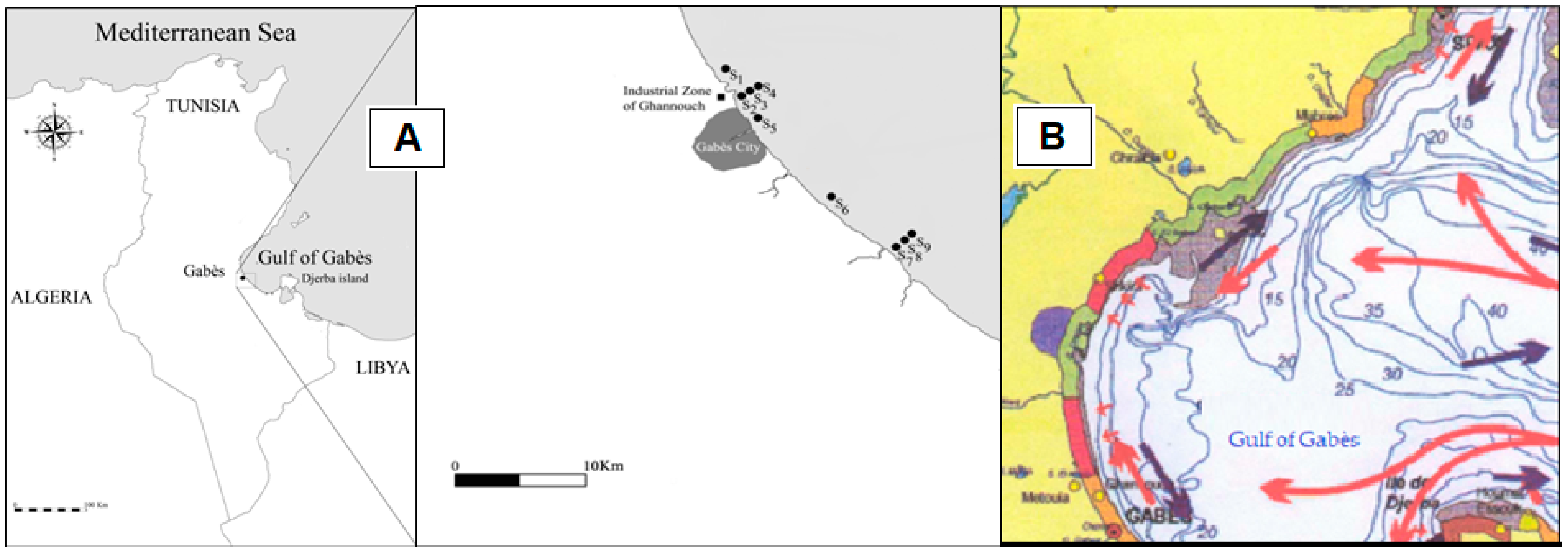
2.1. Study Area
2.2. Sediment Sampling
2.3. Extraction of Carbohydrates
2.4. Trace Metal Analysis
2.5. Fluorine Determination
2.6. Copepod Study
2.7. Data Processing
3. Results
3.1. Abiotic Parameters
3.2. Copepod Parameters
4. Discussion
4.1. Variation of Environmental Variables
4.2. Variation of Meiobenthic Copepod Quantitative Traits from the Gulf of Gabès
4.3. Taxonomic Diversity of Meiobenthic Copepods from Gulf of Gabès
5. Conclusions
Author Contributions
Funding
Institutional Review Board Statement
Informed Consent Statement
Data Availability Statement
Acknowledgments
Conflicts of Interest
References
- IMO (International Maritime Organization). Protocol on Preparedness, Response and Co-operation to Pollution Incidents by Hazardous and Noxious Substances, (OPRC-HNS Protocol). 2000, pp. 1–3. Available online: https://www.iaphworldports.org (accessed on 17 November 2022).
- HASREP. Report on Task 1: Monitoring of the Flow of Chemicals Transported by Sea in Bulk; Publications Office of The European Union Luxembourg: Luxembourg, 2005; p. 125. [Google Scholar]
- Nieboer, E.; Richardson, D.H.S. The replacement of the nondescript term heavy metals by a biologically and chemically significant classification of metal ions. Environ. Pollut. B 1980, 1, 3–26. [Google Scholar] [CrossRef]
- Velez, D.; Montoro, R. Arsenic speciation in manufactured seafood products: A review. J. Food Protect. 1998, 61, 1240–1245. [Google Scholar] [CrossRef] [PubMed]
- Conacher, H.B.; Page, B.D.; Ryan, J.J. Industrial chemical contamination of foods [Review]. Food Addit. Contam. 1993, 10, 129–143. [Google Scholar] [CrossRef] [PubMed]
- Demirak, A.; Yilmaz, F.; Tuna, A.L.; Ozdemir, N. Heavy metals in water, sediment and tissues of Leuciscus cephalus from a stream in southwestern Turkey. Chemosphere 2006, 63, 1451–1458. [Google Scholar] [CrossRef]
- Khaled, A.; Nemr, A.E.; Sikaily, A.E. An assessment of heavy metal contamination in surface sediments of the Suez Gulf using geoaccumulation indexes and statistical analysis. Chem. Ecol. 2006, 22, 239–252. [Google Scholar] [CrossRef]
- Singh, K.P.; Mohan, D.; Singh, V.K.; Malik, A. Studies on distribution and fractionation of heavy metals in Gomti river sediments-atributary of the Ganges. J. Hydrol. 2005, 312, 14–27. [Google Scholar] [CrossRef]
- Ghrefat, H.; Yusuf, N. Assessing Mn, Fe, Cu, Zn, and Cd pollution in bottom sediments of Wadi Al-Arab Dam Jordan. Chemosphere 2006, 65, 2114–2121. [Google Scholar] [CrossRef]
- CGP. Annuaire des Statistiques des Pêches en Tunisie; Ministère de l’Agriculture: Tunis, Tunisie, 1996; p. 130.
- D’Ortenzio, F.; d’Alcalà, M.R. On the trophic regimes of the Mediterranean Sea: A satellite analysis. Biogeosciences 2009, 6, 139–148. [Google Scholar] [CrossRef]
- Béjaoui, B.; Ismail, S.B.; Othmani, A.; Hamida, O.B.A.-B.H.; Chevalier, C.; Feki-Sahnoun, W.; Harzallah, A.; Hamida, N.B.H.; Bouaziz, R.; Dahech, S. Synthesis review of the Gulf of Gabès (eastern Mediterranean Sea, Tunisia): Morphological, climatic, physical oceanographic, biogeochemical and fisheries features. Coast. Shelf Sci. 2019, 219, 395–408. [Google Scholar] [CrossRef]
- Bradai, M.N.; Quignard, J.P.; Bouain, A.; Jarboui, O.; Ouannes-Ghorbel, A.; Ben Abdallah, L.; Zaouali, J.; Ben Salem, S. Ichtyofaune autochtone et exotique des côtes tunisiennes: Recensement et biogéographie. Cybium 2004, 28, 315–328. [Google Scholar]
- Zaouali, J. Les peuplements benthiques de la petite Syrte, golfe de Gabès Tunisie. Résultats de la campagne de prospection du mois de juillet 1Etude préliminaire: Biocénoses et thanatocénoses récentes. Mar. Life 1993, 3, 47–60. [Google Scholar]
- Bejaoui, B.; Rais, S.; Koutitonsky, V. Modélisation de la dispersion du phosphogypse dans le golfe de Gabès. Bull. Inst. Natl. Sci. Technol. Mer Salammbô 2004, 31, 103–109. [Google Scholar]
- Hamza-Chaffai, A.; Amiard-Triquet, C.; El Abed, A. Metallothionein-Like Protein: Is It an Efficient Biomarker of Metal Contamination? A Case Study Based on Fish from the Tunisian. Coast. Arch. Environ. Contam. Toxicol. 1997, 33, 53–62. [Google Scholar] [CrossRef]
- Zairi, M.; Rouis, M.J. Impacts environnementaux du stockage du phosphogypse à Sfax (Tunisie). Bull. Lab. Ponts Chaussées 1999, 29–40. [Google Scholar]
- Bradai, M.N. Diversité du Peuplement Ichtyque et Contribution à la Connaissance des Sparidés du Golfe de Gabès. Ph.D. Thesis, Faculté des Sciences de Sfax Université de Sfax Tunisie, Sfax, Tunisia, 2000; p. 595. [Google Scholar]
- Bradai, M.N.; Ghorbel, M.; Bouain, A.; Jarboui, O.; Ouannes-Ghorbel, A.; Mnif, L. La Pêche Côtière dans le Gouvernorat de Sfax, Aspect Socio-Économique et Technique: Ecologie de certains Poissons; Rapport pour la Fondation de la Recherche Scientifique; Faculté des Sciences de Sfax Université de Sfax Tunise: Sfax, Tunisia, 1995; p. 94. [Google Scholar]
- Guillaumont, B.; Ben Mustapha, S.; Ben Moussa, H.; Zaouali, J.; Soussi, N.; Ben Mammou, A.; Cariou, C. Pollution impact study in Gabes Gulf (Tunisia) using remote sensing data. Mar. Technol Soc. J. 1995, 29, 46–58. [Google Scholar]
- Anonymous. Problèmes prioritaires pour l’environnement méditerranéen. Rapp. AEE 2006, 4, 92. [Google Scholar]
- Ben Mustapha, K.; Hattour, A. Les herbiers de posidonies du littoral tunisien I. Le golfe de Hammamet. Notes Inst. Natl. Sci. Technol. Océanogr. Pêche Salammbô 1992, 2, 1–42. [Google Scholar]
- Hamza, A.; Ben Maïz, N. Sur l’apparition du phénomène “d’eau rouge” dans le Golfe de Gabès (Tunisie) en été 1. Bull. Inst. Natl. Sci. Technol. Océanogr. Pêche Salammbô 1990, 17, 5–16. [Google Scholar]
- Hamza, A. Contribution à l’étude des phytoplanctons et des phénomènes d’eutrophisation algale dans le golfe de Gabès. DEA Master Degree Faculté Sciences Sfax Université Sfax 1997, 120. [Google Scholar]
- Sfar Felfoul, H.; Clastres, P.; Ben Ouezdou, M.; Carles-Gibergues, A. Properties and perspectives of valorization of phosphogypsum the example of Tunisia. In Proceedings of the International Symposium on Environmental Pollution Control and Waste Management, Tunis, Tunisia, 7–10 January 2002; pp. 510–520. [Google Scholar]
- Ben Brahim, M.; Hamza, A.; Hannachi, I.; Rebai, A.; Jarboui, O.; Bouain, A.; Aleya, L. Variability in the structure of epiphytic assemblages of Posidonia oceanica in relation to human interferences in the Gulf of Gabès, Tunisia. Mar. Environ. Res. 2010, 70, 411–421. [Google Scholar] [CrossRef]
- Bellair, P.; Pomerol, C. Eléments de Géologie, 5th ed.; Colin: Paris, France, 1977; Volume 1, 528p. [Google Scholar]
- Hedfi, A.; Ben Alia, M.; Hassana, M.M.; Albogamia, B.; Al-Zahrania, S.S.; Mahmoudi, E.; Karachled, K.P.; Rohal-Lupher, M.; Boufahja, F. Nematode traits after separate and simultaneous exposure to Polycyclic Aromatic Hydrocarbons (anthracene, pyrene and benzo[a]pyrene) in closed and open microcosms. Environ. Pollut. 2021, 276, 116759. [Google Scholar] [CrossRef] [PubMed]
- Amorri, J.; Geffroy-Rodier, C.; Boufahja, F.; Mahmoudi, E.; Aïssa, P.; Ksibi, M.; Amblès, A. Organic matter compounds as source indicators and tracers for marine pollution in a western Mediterranean coastal zone. Environ. Sci. Pollut. Res. 2011, 18, 1606–1616. [Google Scholar] [CrossRef] [PubMed]
- McCall, J.N.; Fleeger, J.W. Predation by juvenile fish on hyperbenthic meiofauna: A review with data on post-larval Leiostomus xanthurus. Vie Milieu 1995, 45, 61–73. [Google Scholar]
- Bodiou, J.Y. Modalités de la prédation des copépodes benthiques par les poissons. Vie Milieu 1999, 49, 303–308. [Google Scholar]
- Keller, M. Influence du rejet en mer de l’égout de Marseille sur les peuplements du méiobenthos. Ph.D. Thesis, Thèse 3 ème cycle, Uni. Aix-Marseille II, Marseille, France, 1984; p. 131. [Google Scholar]
- Webb, G.D.; Montagna, A.P. Reproductive patterns in meiobenthic Harpacticoida (Crustacea, Copepoda) of the California continental shelf (Santa Maria Basin). Conti. Shel. Res. 1993, 13, 723–739. [Google Scholar] [CrossRef]
- Street, G.T.; Montagna, P.A. Loss of genetic diversity in Harpacticoida near offshore platforms. Mar. Biol. 1996, 126, 271–282. [Google Scholar] [CrossRef]
- Moore, C.G.; Stevenson, J.M. A possible new meiofaunal tool for assessment of the environmental impact of marine oil pollution. Cah. Biol. Mar. 1997, 38, 277–282. [Google Scholar]
- Barka, S.; Forget, J.; Menasria, M.R.; Pavillon, J.F. Le copépode Harpacticoïde Tigriopus brevicornis (Müller) peut-il être considéré comme une sentinelle de la qualité de l’environnement dans la zone supra-littorale? J. Rech. Océanol. 1998, 23, 131–138. [Google Scholar]
- Street, G.T.; Lotufo, G.R.; Montagna, P.A.; Fleeger, J.W. Reduced genetic diversity in a meiobentic copepod exposed to a xenobiotic. J. Exper. Mar. Biol. Ecol. 1998, 222, 93–111. [Google Scholar] [CrossRef]
- Kovatch, C.E.; Chandler, T.G.; Coull, B.C. Utility of a full life-cycle copepod bioassay approach for assessement of sediment associated contaminant mixtures. Mar. Pollut. Bull. 1999, 38, 692–701. [Google Scholar] [CrossRef]
- Mu, F.H.; Somerfield, P.J.; Warwick, R.M.; Zhang, Z.N. Large-scale spatial patterns in the community structure of Benthic harpacticoid copepods in the Bohai sea, China. Raffles Bull. Zoolog. 2002, 50, 17–26. [Google Scholar]
- Rose, A.; Seifried, S. Small-scale diversity of Harpacticoida (Crustacea, Copepoda) from an intertidal sandflat in the Jade bay (German Bight, North Sea). Senckenb. Marit. 2006, 36, 109–122. [Google Scholar] [CrossRef]
- Gheerardyn, H.; De Troch, M.; Ndaro, S.G.M.; Raes, M.; Vincx, M.; Vanreusel, A. Community structure and microhabitat preferences of harpacticoid copepods in a tropical reef lagoon (Zanzibar Island, Tanzania). J. Mar. Biol. Ass. UK 2008, 88, 747–758. [Google Scholar] [CrossRef]
- Heip, C.H.R.; Vincx, M.; Vranken, G. The ecology of marine nematodes. In Oceanography and Marine Biology: An Annual Review; Aberdeen University Press/Allen & Unwin: London, UK, 1985. [Google Scholar]
- Schratzberger, M.; Gee, J.M.; Rees, H.L.; Boyd, S.E.; Wall, C.M. The structure and taxonomic composition of sublittoral meiofauna assemblages as an indicator of the status of marine environments. J. Mar. Biol. Ass. UK 2000, 80, 969–980. [Google Scholar] [CrossRef]
- Pacioglu, O.; Robertson, A. The invertebrate community of the chalk stream hyporheic zone: Spatio-temporal distribution patterns. Knowl. Manag. Aqua. Ecosys. 2017, 418, 10. [Google Scholar] [CrossRef][Green Version]
- Pacioglu, O.; Pârvulescu, L. The chalk hyporheic zone: A true ecotone? Hydrobiologia 2017, 790, 1–12. [Google Scholar] [CrossRef]
- Lang, K. Monographie der Harpacticiden; Håkan Ohlsson Boktryckeri: Lund, Sweeden, 1948; pp. 1–1683. [Google Scholar]
- Hicks, G.R.F.; Coull, B.C. The ecology of marine meiobenthic harpacticoid copepods. Oceanogr. Mar. Biol. Ann. Rev. 1983, 21, 67–175. [Google Scholar]
- Coull, B.C.; Chandler, G.T. Pollution and meiofauna: Field, laboratory, and mesocosm studies. Oceanogr. Mar. Biol. Ann. Rev. 1992, 30, 191–271. [Google Scholar]
- McLachlan, A.; Brown, A.C. The Ecology of Sandy Shores, 2nd ed.; Elsevier Science: Amsterdam, The Netherlands, 2006. [Google Scholar]
- Folkers, C.; George, K.H. Community analysis of sublittoral Harpacticoida (Copepoda, Crustacea) in the western Baltic Sea. Hydrobiologia 2011, 666, 11–20. [Google Scholar] [CrossRef]
- Chertoprud, E.S.; Gheerardyn, H.; Gómez, S. Harpacticoida (Crustacea: Copepoda) of the South China Sea: Faunistic and biogeographical analysis. Hydrobiologia 2011, 666, 45–57. [Google Scholar] [CrossRef]
- Veit-Köhler, G.; Laudien, J.; Knott, J.; Velez, J.; Sahade, R. Meiobenthic colonisation of soft sediments in arctic glacial Kongsfjorden (Svalbard). J. Exp. Mar. Biol. Ecol. 2008, 363, 58–65. [Google Scholar] [CrossRef]
- Veit-Köhler, G.; Gerdes, D.; Quiroga, E.; Hebbeln, D.; Sellanes, J. Metazoan meiofauna within the oxygen-minimum zone off Chile: Results of the 2001-PUCK expedition. Deep-Sea Res. II 2009, 56, 1105–1111. [Google Scholar] [CrossRef]
- Pacioglu, O.; Duţu, F.; Pavel, A.B.; Duţu, L.T. The influence of hydrology and sediment grain-size on the spatial distribution of macroinvertebrate communities in two submerged dunes from the Danube Delta (Romania). Limnetica 2022, 41, 85–100. [Google Scholar] [CrossRef]
- Noli, N.; Sbrocca, C.; Sandulli, R.; Balsamo, M.; Semprucci, F. Contribution to the knowledge of meiobenthic Copepoda (Crustacea) from the Sardinian coast, Italy. Arx. Miscel·Lània Zoològica 2018, 16, 121–133. [Google Scholar] [CrossRef]
- Razouls, C. Les Copépodes Libres; Musée Océanographique de Monaco: Monaco, Monaco, 1988. [Google Scholar]
- Huys, R.; Gee, J.M.; Moore, C.G.; Hamond, R. Marine and Brackish Water Harpacticoid Copepods (Part 1); Synopses of the British Fauna (New, Series); Barnes, R.S.K., Crothers, J.H., Eds.; The Linnean Society of London: London, UK, 1996; Volume 51, p. 352. [Google Scholar]
- Boufahja, F.; Vitiello, P.; Aïssa, P. More than 35 years of studies on marine nematodes from Tunisia: A checklist of species and their distribution. Zootaxa 2014, 3786, 269–300. [Google Scholar] [CrossRef]
- Allouche, M.; Ishak, S.; Ben Ali, M.; Hedfi, A.; Almalki, M.; Karachle, P.K.; Harrath, A.H.; Abu-Zied, R.H.; Badraoui, R.; Boufahja, F. Molecular interactions of polyvinyl chloride microplastics and beta-blockers (diltiazem and bisoprolol) and their effects on marine meiofauna assessed through taxonomy and functional traits: Combined in vivo and modeling study. J. Hazard. Mater. 2022, 431, 128609. [Google Scholar] [CrossRef]
- Monard, A. Les Harpacticoïdes marins de la région de Salammbô. Tunis. Bull. Inst. Natl. Sci. Tech. Oceanogr. Peche. Salammbo 1935, 34, 94. [Google Scholar]
- Amorri, J.; Veit-Köhler, G.; Drewes, J.; Aïssa, P. Apodopsyllus gabesensis n. sp.: A new species of Paramesochridae (Copepoda: Harpacticoida) from the Gulf of Gabès (south-eastern Tunisia). Helgol. Mar. Res. 2010, 64, 191–203. [Google Scholar] [CrossRef][Green Version]
- Amorri, J. Contribution à l’étude des Copépodes Benthiques de la Lagune de Bizerte. Master’s Thesis, Faculté des Sciences de Bizerte, Zarzouna, Tunisia, 2004; p. 152. [Google Scholar]
- Daly Yahia, M.N. Contribution à l’étude du Milieu et du Zooplancton de la Lagune de BouGhrara: Systématique, Biomasse et Relations Trophiques. Master’s Thesis, Faculté des Sciences de Tunis Université de Tunis II, Tunis, Tunisia, 1993; p. 156. [Google Scholar]
- Daly Yahia, M.; Romdhane, M. Dynamique trophique du Zooplancton et relation Phytoplancton-Zooplancton au sein de l’écosystème de la mer de Bou Grara. Bull Inst. Natl. Sci. Technol. Mer Salammbô 1994, 21, 47–65. [Google Scholar]
- Daly Yahia, M.; Romdhane, M. Contribution à la connaissance des cycles saisonnières du zooplancton de la mer de Boughrara (Ensemble de la commuté zooplanctonique). Rev. L’inat 1996, 11, 7–27. [Google Scholar]
- Souissi, S.; Yahia-Kéfi, O.D.; Yahia, M.D. Spatial characterization of nutrient dynamics in the Bay of Tunis (south-western Mediterranean) using multivariate analyses: Consequences for phyto-and zooplankton distribution. J. Plankton Res. 2000, 22, 2039–2059. [Google Scholar] [CrossRef]
- Daly Yahia, M.N.; Souissi, S.; Daly Yahia Kefi, O. Spatial and temporal structure of planktonic copepods in the Bay of Tunis (southwestern Mediterranean Sea). Zool. Stud. 2004, 43, 366–375. [Google Scholar]
- Souissi, A.; Souissi, S.; Yahia, M.N.D. Temporal variability of abundance and reproductive traits of Centropages kroyeri (Calanoida; Copepoda) in Bizerte Channel (SW Mediterranean Sea, Tunisia). J. Exp. Mar. Biol. Ecol. 2008, 355, 125–136. [Google Scholar] [CrossRef]
- Touzri, C.; Kéfi-Daly Yahia, O.; Hamdi, H.; Goy, J.; Yahia, M.N.D. Spatio-temporal distribution of Medusae (Cnidaria) in the Bay of Bizerte (South Western Mediterranean Sea). Cah. Biol. Mar. 2010, 51, 167–176. [Google Scholar]
- Touzri, C.; Hamdi, H.; Goy, J.; Daly Yahia, M.N. Diversity and distribution of gelatinous zooplankton in the Southwestern Mediterranean Sea. Mar. Ecol. 2012, 33, 393–406. [Google Scholar] [CrossRef]
- Neffati, N.; Daly Yahia-Kefi, O.; Bonnet, D.; Carlotti, F.; Daly Yahia, M.N. Reproductive traits of two calanoid copepods: Centropages ponticus and Temora stylifera, in autumn in Bizerte Channel. J. Plankton Res. 2013, 35, 80–96. [Google Scholar] [CrossRef]
- Drira, Z.; Bel Hassen, M.; Ayadi, H.; Aleya, L. What factors drive copepod community distribution in the Gulf of Gabès, Eastern Mediterranean Sea? Environ. Sci. Pollut. Res. 2014, 214, 2918–2934. [Google Scholar] [CrossRef]
- Ben Lamine, Y.; Pringault, O.; Aissi, M.; Ensibi, C.; Mahmoudi, E.; Kefi, O.D.Y.; Yahia, M.N.D. Environmental controlling factors of copepod communities in the Gulf of Tunis (south western Mediterranean Sea). Cah. Biol. Mar. 2015, 56, 213–229. [Google Scholar]
- Ben Ltaief, T.; Drira, Z.; Devenon, J.L.; Hamza, A.; Ayadi, H.; Pagano, M. How could thermal stratification affect horizontal distribution of depth-integrated metazooplankton communities in the Gulf of Gabes (Tunisia)? Mar. Biol. Res. 2017, 13, 269–287. [Google Scholar] [CrossRef]
- Ben Ltaief, T.; Drira, Z.; Hannachi, I.; Hassen, M.B.; Hamza, A.; Pagano, M.; Ayadi, H. What are the factors leading to the success of small planktonic copepods in the Gulf of Gabès, Tunisia? J. Mar. Biol. Assoc. United Kingd. 2015, 95, 747–761. [Google Scholar] [CrossRef]
- Makhlouf Belkahia, N.; Pagano, M.; Chevalier, C.; Devenon, J.L.; Yahia, M.N.D. Zooplankton abundance and community structure driven by tidal currents in a Mediterranean coastal lagoon (Boughrara, Tunisia, SW Mediterranean Sea). Estuar. Coast. Shelf Sci. 2021, 250, 107101. [Google Scholar] [CrossRef]
- Beyrem, H.; Aïssa, P. Les nématodes libres, organismes sentinelles de l’évolution des concentrations d’hydrocarbures dans la baie de Bizerte (Tunisie). Cah. Biol. Mar. 2000, 41, 329–342. [Google Scholar]
- Hermi, M.; Aïssa, P. Structure printanière des peuplements nématologiques de la lagune Sud de Tunis (Tunisie). Mar. Life 2002, 12, 27–36. [Google Scholar]
- Mahmoudi, E.; Essid, N.; Beyrem, H.; Hedfi, A.; Boufahja, F.; Vitiello, P.; Aissa, P. Effects of hydrocarbon contamination on a freeliving marine nematode community: Results from microcosm experiments. Mar. Pollut. Bull. 2005, 50, 1197–1204. [Google Scholar] [CrossRef]
- Hedfi, A.; Mahmoudi, E.; Boufahja, F.; Beyrem, H.; Aïssa, P. Effects of increasing levels of nickel contamination on structure of offshore nematode communities in experimental microcosms. Bull. Environ. Contam Toxicol. 2007, 79, 345–349. [Google Scholar] [CrossRef]
- Beyrem, H.; Mahmoudi, E.; Essid, N.; Hedfi, A.; Boufahja, F.; Aïssa, P. Individual and combined effects of cadmium and diesel on a nematode community in a laboratory microcosm experiment. Ecotoxicol. Environ. Saf. 2007, 68, 412–418. [Google Scholar] [CrossRef]
- Sun, B.; Fleeger, J.W. Sustained mass culture of Amphiascoides atopus, a marine harpacticoid copepod, in a recirculated system. Aquaculture 1995, 136, 313–321. [Google Scholar] [CrossRef]
- Chandler, G.T.; Cary, T.L.; Volz, T.C.; Walse, S.S. Fipronil effects on the estuarine copepod (Amphiascus tenuiremis) development, fertility, and reproduction: A rapid life-cycle assay in 96-well microplate format. Environ. Toxicol. Chem. 2004, 23, 117–124. [Google Scholar] [CrossRef]
- Aïssa, P. Ecologie des Nématodes Libres de la Lagune de Bizerte: Dynamique et Biocénotique. Ph.D. Thesis, Faculté des Sciences de Tunis Université de Tunis, Tunis, Tunisia, 1991; p. 370. [Google Scholar]
- Hermi, M. Les nématodes libres: Bio-indicateurs des conditions physico-chimiques de deux lagunes tunisiennes (lagune de Bizerte et lagune de Tunis). Master’s Thesis, Faculté des Sciences de Tunis, Université de Tunis, Tunis, Tunisia, 1995; p. 134. [Google Scholar]
- Beyrem, H. Ecologie des Nématodes Libres de Deux Milieux Anthropiquement Perturbés: La Baie de Bizerte et le lac Ichkeul. Ph.D. Thesis, Faculté des Sciences de Bizerte Université de Carthage, Zarzouna, Tunisia, 1999; p. 297. [Google Scholar]
- Hedfi, A. Etat de pollution du vieux port de Bizerte et impact sur le méiobenthos. Master’s Thesis, Faculté des Sciences de Bizerte Université des Carthage, Zarzouna, Tunisia, 2003; p. 105. [Google Scholar]
- Mahmoudi, E. La méiofaune de deux lagunes perturbées: Ghar El Melh et Bou Ghrara. Ph.D. Thesis, Faculté des Sciences de Bizerte, Université de Carthage, Zarzouna, Tunisia, 2003; p. 334. [Google Scholar]
- Sammari, C.; Koutitonsky, V.G.; Moussa, M. Sea level variability and tidal resonance in the Gulf of Gabes, Tunisia. Cont. Shelf Res. 2006, 26, 338–350. [Google Scholar] [CrossRef]
- Hattour, M.J.; Sammari, C.; Ben Nassrallah, S. Hydrodynamique du golfe de Gabès déduite à partir des observations de courants et de niveaux. Rev. Paralia 2010, 3, 3.1–3.12. [Google Scholar] [CrossRef]
- Anonymous. Etude d’impact sur l’environnement de l’usine projetée d’acide phosphorique tifert dans le site de la Skhira. Rapport GEREP- Environ. 2007, 250. [Google Scholar]
- Ghorbel, M. Le pageot commun Pagellus erythrinus (Poisson, Sparidae). Ecobiologie et état d’exploitation dans le golfe de Gabès. Ph.D. Thesis, Faculté des Sciences de Sfax, Université de Sfax, Sfax, Tunisia, 1996; p. 170. [Google Scholar]
- Gruvel, A. L’industrie des pêches sur les cotes tunisiennes. Bull. Inst. Natl. Sci. Technol. Océanogr. Pêche Salammbô 1926, 4, 1–135. [Google Scholar]
- Ben Othmen, S. Le sud tunisien (golfe de Gabès), hydrologie, sédimentologie, flore et faune. Ph.D. Thesis, Faculté des Sciences de Tunis Université de Tunis, Tunis, Tunisia, 1973; p. 166. [Google Scholar]
- Ben Othmen, S. Observation hydrologiques, dragages et chalutage dans le Sud-est tunisien. Bull. Inst. Natl. Sci. Technol. Océanogr. Pêche Salammbô 1971, 2, 103–120. [Google Scholar]
- Perès, J.M.; Picard, J. Nouveau manuel de bionomie benthique de la Méditerranée. Rec. Trav. Str. Mar. Endoume 1965, 22, 5–15. [Google Scholar]
- De Gaillande, D. Peuplements benthiques de l’herbier de Posidonia oceanica Delile et de la pelouse à Caulerpa prolifera Amouroux du large du golfe de Gabès. Tethys 1970, 2, 373–384. [Google Scholar]
- Ktari-Chakroun, F.; Azouz, A. Les fonds chalutables de la région sud-est de la Tunisie (golfe de Gabès). Bull. Inst. Océanogr Pêche Salammbô 1971, 2, 5–48. [Google Scholar]
- Molinier, R.; Picard, J. Elément de bionomie marine sur les côtes de la Tunisie. Bull. Sta. Océanogr. Salammbô 1954, 48, 1–47. [Google Scholar]
- Buchanan, J.B. Sediments. In Measurement of the Physical and Chemical Environment; Buchanan, J.B., Kain, J.M., Eds.; Blackwell Sciences: Oxford, UK, 1971; pp. 30–52. [Google Scholar]
- Hakkarainen, M.; Albertsson, A.C.; Karlsson, S. Solid phase extraction and subsequent gas chromatography-mass spectrophotometry analysis for identification of complex mixtures of degradation production starch-based polymers. J. Chromatogr. A 1996, 741, 251–263. [Google Scholar] [CrossRef]
- Poulain, M. Structure et Dynamique du Carbone Organique dans les Milieux Aqueux: Relations sédiment/eau. Ph.D. Thesis, Université de Poitiers, Poitiers, France, 2005; p. 200. [Google Scholar]
- Loring, D.H.; Rantala, R.T.T. Sediment and suspended particulate matter: Total and partial methods of digestion ICE Tech. Mar. Environ. Sci. 1990, 9, 14. [Google Scholar]
- UNEP/IAEA/FAO. Determination of total cadmium, zinc, lead and copper in selected marine organisms by atomic absorption spectrophotometry. Ref. Methods Mar. Pollut. Stud. N° 11 Rev. 1984, 1, 1–21. [Google Scholar]
- McQuaker, N.R.; Gurney, M. Determination of total fluoride in soil and vegetation using an alkali fusion selective ion electrode technique. Anal. Chem. 1977, 49, 53–56. [Google Scholar] [CrossRef]
- Vivier, M.H. Influence d’un déversement industriel profond sur la nématofaune (Canyon de Cassidaigne, Méditerranée). Tethys 1978, 8, 307–321. [Google Scholar]
- Guo, Y.; Somerfield, P.J.; Warwick, R.M.; Zhang, Z. Large-scale patterns in the community structure and biodiversity of free-living nematodes in the Bohai Sea, China. J. Mar. Biol. Ass. UK 2001, 81, 755–763. [Google Scholar] [CrossRef]
- Bodin, P. Catalogue of the new marine Harpacticoid Copepods. Document de travail. Inst. R. Sci. Nat. Belg. 1997, 89, 304. [Google Scholar]
- Boxshall, G.; Halsey, S.H. An Introduction to Copepod Diversity; The Ray Society Series; Ray Society: London, UK, 2004; p. 966. [Google Scholar]
- Warwick, R.M.; Gee, J.M. Community structure of estuarine meiobenthos. Mar. Ecol. Prog. Ser. 1984, 18, 97–111. [Google Scholar] [CrossRef]
- Moran, P.A.P. Notes on Continuous Stochastic Phenomena. Biometrika 1950, 37, 17–23. [Google Scholar] [CrossRef]
- Oden, N.L.; Sokal, R.R. Directional Autocorrelation: An Extension of Spatial Correlograms to Two Dimensions. Syst. Zool. 1986, 35, 608–617. [Google Scholar] [CrossRef]
- Legendre, P.; Fortin, M.J. Spatial pattern and ecological analysis. Vegetatio 1989, 80, 107–138. [Google Scholar] [CrossRef]
- Oden, N.L. Assessing the significance of a spatial correlogram. Geogr. Anal. 1984, 1–16. [Google Scholar] [CrossRef]
- Cressie, N.A.C. Statistics for Spatial Data; Wiley Interscience Publications: New York, NY, USA, 1993; p. 887. [Google Scholar]
- Lichstein, J.W.; Simons, T.R.; Shriner, S.A.; Franzreb, K.E. Spatial autocorrelation and autoregressive models in ecology. Ecol. Monogr. 2002, 72, 445–463. [Google Scholar] [CrossRef]
- Rangel, T.F.; Diniz-Filho, J.A.F.; Bini, L.M. SAM: A comprehensive application for Spatial Analysis in Macroecology. Ecography 2010, 33, 2010. [Google Scholar] [CrossRef]
- Frisoni, G.F.; Guelorget, O.; Pertuisot, J.P.; Fresi, E. Diagnose Écologique et Zonation biologique du lac de Bizerte. In Applications aquacoles: Rapport du projet MEDRAP: Regional Mediterranean Developpement of Aquaculture; FAO DIT/86/03/IPCM/Brest; FAO: Paris, France, 1986; 41p. [Google Scholar]
- Venkatesan, M.I.; Ruth, E.; Steinberg, S.; Kaplan, I.R. Organic geochemistry of sediments from the continental margin off southern New England. USA: Part II. Lipids. Mar. Chem. 1987, 21, 267–299. [Google Scholar] [CrossRef] [PubMed]
- Volkman, J.K.; Holdsworth, D.G.; Neill, G.P.; Bavor, H.J. Identification of natural, anthropogenic and petroleum hydrocarbons in aquatic sediments. Sci. Total Environ. 1992, 112, 203–219. [Google Scholar] [CrossRef] [PubMed]
- Louati, A.; Elleuch, B.; Kallel, M.; Oudot, J.; Saliot, A.; Dagaut, J. Hydrocarbon contamination of coastal sediments from the Sfax area (Tunisia), Mediterranean Sea. Mar. Pollut. Bull. 2001, 42, 445–452. [Google Scholar] [CrossRef]
- Zaghden, H.; Kallel, M.; Louati, A.; Elleuch, B.; Oudot, J.; Saliot, A. Hydrocarbons in surface sediments from the Sfax coastal zone, (Tunisia) Mediterranean Sea. Mar. Pollut. Bull. 2005, 50, 1287–1294. [Google Scholar] [CrossRef]
- Farrington, J.W.; Tripp, B.W. Hydrocarbons in western North Atlantic surface sediments. Geochim. Cosmochim. Acta 1977, 41, 1627–1641. [Google Scholar] [CrossRef]
- Grimalt, J.O.; Albaiges, J. Characterization of the depositional environments of the Ebro Delta western Mediterranean by the study of sedimentary lipid markers. Mar. Geol. 1990, 95, 207–224. [Google Scholar] [CrossRef]
- Lipiatou, E.; Saliot, A. Hydrocarbon contamination of the Rhone delta and the open western Mediterranean. Mar. Pollut. Bull. 1991, 22, 297–304. [Google Scholar] [CrossRef]
- Aboul-Kassim, T.A.T.; Simoneit, B.R.T. Aliphatic and aromatic hydrocarbons in particulate fallout of Alexandria, Egypt: Sources and implications. Environ. Sci. Technol. 1995, 29, 2473–2483. [Google Scholar] [CrossRef]
- Tolosa, I.; Bayona, J.M.; Albaiges, J. Aliphatic and polycyclic aromatic hydrocarbons and sulfur/oxygen derivatives in Northwestern Mediterranean sediments: Spatial and temporal variability fluxes and budgets. Environ. Sci. Technol. 1996, 30, 2495–2503. [Google Scholar] [CrossRef]
- Wakeham, S.G. Aliphatic and polycyclic aromatic hydrocarbons in Black Sea sediments. Mar. Chem. 1996, 53, 187–205. [Google Scholar] [CrossRef]
- Gogou, A.; Bouloubassi, I.; Stephanou, E.G. Marine organic geochemistry of the Eastern Mediterranean: 1. Aliphatic and polyaromatic hydrocarbons in Cretan Sea superficial sediments. Mar. Chem. 2000, 68, 265–282. [Google Scholar] [CrossRef]
- Brassell, S.C.; Eglinton, G. Natural and pollutant organic compounds in contemporary aquatic environments. In Analytical Techniques in Environmental Chemistry; Albaigés, J., Ed.; Pergamon Press: Oxford, UK, 1980; pp. 1–22. [Google Scholar]
- Saliot, A. Natural hydrocarbons in seawater. In Marine Organic Chemistry. Pollution Evolution, Composition, Interactions and Chemistry of Organic Matter in Seawater; Duursma, E.K., Dawson, R., Eds.; Elsevier: Amsterdam, The Netherlands, 1981; pp. 327–374. [Google Scholar]
- Kvenvolden, K.A.; Rapp, J.B.; Golan-Bac, M.; Hostettler, F.D. Multiple sources of alkanes in quaternary oceanic sediment of Antarctica. Org. Geochem. 1987, 11, 291–302. [Google Scholar] [CrossRef]
- Wang, Z.; Fingas, M.F. Development of oil hydrocarbon fingerprinting and identification techniques. Mar. Pollut. Bull. 2003, 47, 423–452. [Google Scholar] [CrossRef] [PubMed]
- Sarbaji, M.; Ammar, E.; Bouzid, J.; Saaadate, K.; Medhioub, K. Etude de l’impact des rejets liquides du complexe chimique sur l’environnement marin dans le golfe de Gabès (Tunisie). In Circulation des Eaux et Pollution des Côtes Méditerranéennes des Pays du Maghreb; INOC: Izmir, Turkey, 1993; pp. 157–165. [Google Scholar]
- Zourarah, B.; Carruesco, C.; Labraimi, M.; Reboullon, P.; Bakkas, S. Impact des effluents anthropiques sur les teneurs en métaux lourds dans les sédiments de la lagune de Oualidia (Maroc). Rapp. CIESM 2001, 36, 175. [Google Scholar]
- Ammar, E.; Sassadate, K.; Bouzid, J.; Charfi, M.; Ben Jmaa, M.; Medhioub, K. Impact des rejets industriels du complexe chimique de Ghannouch sur la qualité des eaux marines du golfe de Gabès. In Rapport de l’Agence Nationale de Protection de l’environnement (ANPE); ANPE: Tunis, Tunisia, 1991; p. 120. [Google Scholar]
- Darmoul, B. Recherche sur l’influence des rejets de phosphogypse dans le golfe de Gabès et étude expérimentale de la toxicité. Master’s Thesis, Université De Tunis, Tunis, Tunisia, 1977. [Google Scholar]
- Aubert, M.; Revillon, P.; Gauthier, M. Métaux lourds en Méditerranée; 3éme tome; R.I.O.M.: Nice, France, 1982; p. 171. [Google Scholar]
- MacPherson, C.A.; Chapman, P.M. Copper effects on potential sediment test organisms: The importance of appropriate sensitivity. Mar. Pollut. Bull. 2000, 40, 656–665. [Google Scholar] [CrossRef]
- Hagopian-Schlekat, T.; Chandler, G.T.; Shaw, T.J. Acute toxicity of five sediment-associated metals, individually and in a mixture, to the estuarine meiobenthic harpacticoid copepod Amphiascus tenuiremis. Mar. Environ. Res. 2001, 51, 247–264. [Google Scholar] [CrossRef]
- NOAA. National Oceanic and Atmospheric Administration Screening, Quick Reference Tables (SQuiRTs); Coastal Protection and Restoration Division. Hazardous Materials (HAZMAT) Report; NOAA: Washington, DC, USA, 2004; pp. 1–99.
- El-Said, G.F. Fluoride monitoring in front of some hot spots receiving drainage waters along the Egyptian coastal seawater of Mediterranean during 1996 to 2006. Int. J. Pure Appl. Chem. (IJPAC) 2010, 5, 27–37. [Google Scholar]
- Sarbaji, M.M. Utilisation d’un SIG Multi-Sources Pour la Compréhension et la Gestion Intégrée de L’écosystème Côtier de la Région de Sfax (TUNISIE). Ph.D. Thesis, Faculté des Sciences de Tunis, Université El Manar II Tunis, Tunis, Tunisia, 2000; p. 152. [Google Scholar]
- Camargo, J.A. Fluoride toxicity to aquatic organisms: A review. Chemosphere 2003, 50, 251–264. [Google Scholar] [CrossRef]
- Burns, K.N.; Alicroft, R.; Fluorosisin Cattle, I. Occurrence and Effects in Industrial Areas of England and Wales; MAFF Animal Disease Surveys Report; HMSO: London, UK, 1964; pp. 1954–1957.
- Neumüller, O.A. Römpps Chemie Lexikon, 8th ed.; Franck’sche Verlagshandlung: Stuttgart, Germany, 1981. [Google Scholar]
- Fuge, R. Sources of halogens in the environment, influences on human and animal health. Environ. Geochem. Health 1988, 10, 51–61. [Google Scholar] [CrossRef] [PubMed]
- Fuge, R.; Andrews, M.J. Fluorine in the UK Environ. Environ. Geochem. Health 1988, 96, 104. [Google Scholar]
- WHO. Environmental Health Criteria; World Health Organization: Fluorides, Geneva, 2002; p. 227. [Google Scholar]
- Ramanaiah, S.V.; Venkatamohan, S.; Rajkumar, B.; Sarma, P.N. Monitoring of fluoride concentration in groundwater of Prakasham district in India: Correlation with physico-chemical parameters. J. Environ. Sci. Eng. 2006, 48, 129–134. [Google Scholar]
- Gaciri, S.J.; Davies, T.C. The occurrence and geochemistry of fluoride in some natural waters of Kenya. J. Hydrol. 1993, 143, 395–412. [Google Scholar] [CrossRef]
- Apambire, W.B.; Boyle, D.R. Michel FA Geochemistry, genesis and health implications of fluoriferous groundwater in the upper regions of Ghana. Environ. Geol. 1997, 33, 13–24. [Google Scholar] [CrossRef]
- Fantong, W.Y.; Satake, H.; Aka, F.T.; Ayonghe, S.N.; Asai, K.; Mandal, A.; Ako, A.A. Hydrochemical and isotopic evidence of recharge, apparent age, and flow direction of groundwater in, Mayo Tsanaga River Basin, Cameroon: Bearings on contamination. Environ. Earth Sci. 2010, 60, 107–120. [Google Scholar] [CrossRef]
- WHO. Guidelines for Drinking Water Quality: Health Criteria and Supporting Information; World Health Organization: Geneva, Switzerland, 1984; Volume 2. [Google Scholar]
- Harrison Paul, T.C. Fluoride in water: A UK perspective. J. Fluor. Chem. 2005, 126, 1448–1456. [Google Scholar] [CrossRef]
- Mohapatra, M.; Anand, S.; Mishra, B.K.; Giles, D.E.; Singh, P. Review of Fluoride Removal from drinking water. J. Environ. Manag. 2009, 91, 67–77. [Google Scholar] [CrossRef]
- Lasserre, P.; Renaud-Mornant, J.; Castel, J. Metabolic activities of meiofaunal communities in semi enclosed lagoons: Possibilities of trophic competition between meiofauna and mugilid fish. In Proceedings of the 10th European Symposium on Marine Biology, Ostend, Belgium, 17–23 September 1975; IZWO/Universa Press: Wetteren, Belgium, 1976; pp. 313–414. [Google Scholar]
- Aïssa, P.; Vitiello, P. Impact de la pollution et de la variabilité des conditions ambiantes sur la densité du méiobenthos de la lagune de Tunis. Rev. Fac. Sc. Tunis 1984, 3, 155–177. [Google Scholar]
- Castel, J. Structure et Dynamique des Peuplements de Copépodes dans des Écosystèmes Eutrophes Littoraux (Côte Atlantique). Ph.D. Thesis, Université de Bordeaux I, Bordeaux, France, 1984; p. 336. [Google Scholar]
- Castel, J. Influence de l’activité bioperturbatrice de la palourde (Ruditapes philippinarum) sur les communautés méiobenthiques. C. R. Heb. Acad. Sci. Paris 1984, 229, 761–764. [Google Scholar]
- Fleeger, J.W. Meiofaunal densities and copepod species composition in a Louisiana, USA, estuary. Trans. Am. Microsc. Soc. 1985, 104, 321–332. [Google Scholar] [CrossRef]
- Hodda, M.; Nicholas, W.L. Temporal changes in littoral meiofauna from the Hunter River estuary. Aust. J. Mar. Freshw. Res. 1986, 37, 729–741. [Google Scholar] [CrossRef]
- Alonghi, D.M. Intertidal zonation and sesonality of meiobenthos in tropical mangrove estuaries. Mar. Biol. 1987, 95, 447–458. [Google Scholar] [CrossRef]
- Hermi, M. Impact de la pollution sévissant dans le lac Sud de Tunis sur la méiofaune. Ph.D. Thesis, Faculté des Sciences de Bizerte, Université de Carthage, Carthage, Tunisia, 2001; p. 300. [Google Scholar]
- Saâdallah, S.T. Impact des travaux d’assainissement sur la méiofaune du lac Nord de Tunis. Master’s Thesis, Faculté des Sciences de Bizerte, Université de Carthage, Carthage, Tunisia, 2001; p. 91. [Google Scholar]
- Mouawad, R. Peuplements de Nématodes de la Zone Littorale des Côtes du Liban. Ph.D. Thesis, Université Aix-Marseille II. Centre d’océanologie de Marseille, Marseille, France, 2005; p. 240. [Google Scholar]
- Pacioglu, O.; Shaw, P.; Robertson, A. Patch scale response of hyporheic invertebrates to fine sediment removal in two chalk rivers. Fund. Appl. Limnol. 2012, 181, 283–288. [Google Scholar] [CrossRef]
- Pacioglu, O.; Moldovan, O.T. Response of invertebrates from the hyporheic zone of chalk rivers to eutrophication and land use. Environ. Sci. Pollut. Res. 2016, 23, 4729–4740. [Google Scholar] [CrossRef] [PubMed]
- Pacioglu, O.; Ianovici, N.; Filimon, M.N.; Sinitean, A.; Iacob, G.; Barabas, H.; Alexandru, P.; Acs, A.; Muntean, H.; Pârvulescu, L. The multifaceted effects induced by floods on the macroinvertebrate communities inhabiting a sinking cave stream. Inte. J. Speleol. 2019, 48, 167–177. [Google Scholar] [CrossRef]
- Monard, A. Les Harpacticoïdes marins de la région d’Alger et de Castiglione. Bull. Sta. D’aqui. Pêche Castiglione 1937, 2, 85. [Google Scholar]
- Huys, R.; Boxshall, T.M. Copepod Evolution; The Ray Society: London, UK, 1991; p. 468. [Google Scholar]
- Losi, V.; Montefalcone, M.; Moreno, M.; Giovannetti, E.; Gaozza, L.; Grondona, M.; Albertelli, G. Nematodes as indicators of environmental quality in seagrass (Posidonia oceanica) meadows of the NW Mediterranean Sea. Adv. Ocean. Limnol. 2012, 3, 69–91. [Google Scholar] [CrossRef]
- Semprucci, F.; Sbrocca, C.; Rocchi, M.; Balsamo, M. Temporal changes of the mei ofaunal assemblage as a tool for the assessment of the ecological quality status. J. Mar. Biol. Assoc. United Kingd. 2015, 95, 247–254. [Google Scholar] [CrossRef]
- Monard, A. Note préliminaire sur les Harpacticoïdes marins d’Alger. Bulletin Station Aquiculture Pêche Castiglione 1936, 1, 41. [Google Scholar]
- Coull, B.C.; Dudley, B.W. Dynamics of meiobenthic copepod populations: A long-term study (1973–1983). Mar. Ecol. Prog. Ser. 1985, 24, 219–229. [Google Scholar] [CrossRef]
- Ouakad, M. Caractères sédimentologiques et géochimiques des dépôts superficiels de la lagune de Bizerte (Tunisie septentrionale). In Circulation des Eaux et Pollution des Côtes Méditerranéennes des Pays du Maghreb; INOC: Izmir, Turkey, 1993; pp. 187–194. [Google Scholar]
- Carman, K.R.; Fleeger, J.W.; Pomarico, S.M. Does historical exposure to hydrocarbon contamination alter the response of benthic communities to diesel contamination? Mar. Environ. Res. 2000, 49, 255–278. [Google Scholar] [CrossRef] [PubMed]
- Bejarano, A.C.; Chandler, T.G.; Decho, A.W. Influence of natural dissolved organic matter (DOM) on acute and chronic toxicity of the pesticides chlorothalonil, chlorpyrifos and fipronil on the meiobenthic estuarine copepod Amphiascus tenuiremis. J. Exp. Mar. Biol. Ecol. 2005, 321, 43–57. [Google Scholar] [CrossRef]
- Millward, R.N.; Carman, K.R.; Fleeger, J.W.; Gambrell, R.P.; Portier, R. Mixtures of metals and hydrocarbons elicit complex responses by a benthic invertebrate community. J. Exp. Mar. Biol. Ecol. 2004, 310, 115–130. [Google Scholar] [CrossRef]
- Barka, S.; Pavillon, J.F.; Amiard, J.C. Influence of different essential and non-essential metals on MTLP levels in the Copepod Tigriopus Brevicornis. Comp. Biochem. Phys. C 2001, 128, 479–493. [Google Scholar] [CrossRef]
- Kovatch, C.E.; Schizas, N.V.; Chandler, G.T.; Coull, B.C.; Quattro, J.M. Tolerance and genetic relatedness of three meiobenthic copepod populations exposed to sediment-associated contaminant mixtures: Role of environmental history. Environ. Toxicol. Chem. 2000, 19, 912–919. [Google Scholar] [CrossRef]
- Bejarano, A.C.; Maruya, K.A.; Chandler, T.G. Toxicity assessment of sediments associated with various land-uses in coastal South Carolina, USA, using a meiobenthic copepod bioassay. Mar. Pollut. Bull. 2004, 49, 23–32. [Google Scholar] [CrossRef]


| Sites | Depth (m) | Latitude (S) | Longitude (W) |
|---|---|---|---|
| S1 | 5 | 33°56′37.14″ | 10° 5′24.88″ |
| S2 | 3 | 33°54′44.37″ | 10° 6′22.02″ |
| S3 | 5 | 33°54′50.56″ | 10° 6′40.96″ |
| S4 | 7 | 33°54′57.98″ | 10° 7′11.57″ |
| S5 | 5 | 33°53′42.57″ | 10° 7′27.66″ |
| S6 | 5 | 33°49′16.23″ | 10°12′17.33″ |
| S7 | 3 | 33°46′13.96″ | 10°16′11.56″ |
| S8 | 5 | 33°46′30.40″ | 10°16′29.83″ |
| S9 | 7 | 33°47′4.59″ | 10°17′7.60″ |
| Sites | Season | Type of Sediment | O2 (mg·L−1) | Carbohydrates (µg/g) | F (g/kg) | Fe (mg/kg) | Cd (mg/kg) | Zn (mg/kg) |
|---|---|---|---|---|---|---|---|---|
| S1 | Winter | Sandy | 7.75 | nd | 2.635 ± 0.361 | 1627 ± 102 | 21.13 ± 2.15 | 213.68 ± 82.11 |
| Spring | Sandy | 7.9 | nd | 2.215 ± 0.945 | 1629.76 ± 93.24 | 22.12 ± 376 | 244.87 ± 34.09 | |
| Summer | Sandy | 7.24 | nd | 2.352 ± 0.672 | 1501.13 ± 167.15 | 21.11 ± 5.04 | 214.86 ± 28.17 | |
| Autumn | Sandy | 6.99 | nd | 2.332 ± 0.428 | 1452.76 ± 305.11 | 21.06 ± 5 | 201 ± 66 | |
| S2 | Winter | Medium silt | 4.09 | 1955 ± 95 | 5.802 ± 1.522 | 5370 ± 258 | 287 ± 16 | 1877 ± 51 |
| Spring | Medium silt | 5.85 | 1707.85 ± 74.2 | 5.813 ± 0.933 | 5371.25 ± 401.23 | 304 ± 12 | 1960 ± 103 | |
| Summer | Medium silt | 5.12 | 442.75 ± 12.5 | 5.815 ± 0.689 | 5403.46 ± 304.71 | 389 ± 35 | 1987.35 ± 216.19 | |
| Autumn | Medium silt | 3.61 | 568.73 ± 36.7 | 5.81 ± 0.721 | 5400 ± 402 | 406.34 ± 62.47 | 1987.65 ± 203.21 | |
| S3 | winter | Medium silt | 3.85 | 367.16 ± 12.94 | 5.778 ± 1.109 | 4484 ± 209 | 473.72 ± 35.68 | 3214 ± 86 |
| spring | Medium silt | 5.95 | 2221.65 ± 18.22 | 5.78 ± 1.451 | 3480 ± 311 | 498.27 ± 62.51 | 3356.4 ± 71.4 | |
| summer | Medium silt | 5.4 | 1082.04 ± 35.02 | 5.714 ± 0.882 | 3500 ± 106 | 512.27 ± 72.04 | 3473.4 ± 63.8 | |
| Autumn | Medium silt | 3.99 | 424 ± 31 | 5.732 ± 1.073 | 4003.5 ± 307.5 | 501.06 ± 18.97 | 3458 ± 107 | |
| S4 | Winter | Silty clay | 4.68 | 3273.45 ± 78.96 | 5.798 ± 1.004 | 6542 ± 405 | 312.03 ± 27.06 | 2014.35 ± 92.61 |
| Spring | Silty clay | 5.75 | 2264.09 ± 108.47 | 5.791 ± 0.952 | 6463.88 ± 109.24 | 304.183 ± 12.54 | 2053.23 ± 64.08 | |
| Summer | Silty clay | 5.35 | 3885.94 ± 98.35 | 5.794 ± 1.307 | 6531.62 ± 307.10 | 312.18 ± 17.82 | 2142.23 ± 70.15 | |
| Autumn | Silty clay | 4.01 | 4379.06 ± 107.08 | 5.796 ± 0.911 | 6567.34 ± 228.19 | 334.68 ± 41.06 | 2131.82 ± 73.11 | |
| S5 | Winter | Silty clay | 4.92 | nd | 0.778 ± 0.082 | 1300.23 ± 89.76 | 22.56 ± 3.84 | 185.06 ± 30.29 |
| Spring | Sandy | 5.69 | nd | 0.732 ± 0.073 | 1440.45 ± 245.08 | 24.5747 ± 4.05 | 198.49 ± 21.08 | |
| Summer | Sandy | 5.52 | nd | 0.731 ± 0.086 | 1321.4 ± 87.51 | 23.5 ± 3.11 | 176.49 ± 15.77 | |
| Autumn | Sandy | 4.98 | nd | 0.745 ± 0.091 | 1123.56 ± 62.88 | 19.17 ± 6.61 | 205.79 ± 36.86 | |
| S6 | Winter | Sandy | 5.76 | 21 ± 4 | 0 | 1234.51 ± 109.05 | 3.21 ± 1.04 | 48.38 ± 8.75 |
| Spring | Sandy | 6.87 | nd | 0 | 1269.41 ± 97.36 | 4.56 ± 1.78 | 51.75 ± 11.09 | |
| Summer | Sandy | 6.49 | 21 ± 2 | 0 | 1231.46 ± 56.44 | 3 ± 1 | 43.75 ± 8.44 | |
| Autumn | Sandy | 6.33 | nd | 0 | 1199.91 ± 102.27 | 3.75 ± 1.10 | 42.89 ± 10.16 | |
| S7 | Winter | Sandy | 8.1 | nd | 0.071 ± 0.020 | 857.65 ± 37.54 | 1 ± 1 | 30.18 ± 6.40 |
| Spring | Sandy | 8.52 | nd | 0.067 ± 0.021 | 945.86 ± 65.10 | 1.59 ± 0.86 | 31.85 ± 8.88 | |
| Summer | Sandy | 7.9 | nd | 0.065 ± 0.003 | 924.85 ± 84.16 | 1 ± 1 | 29.85 ± 7.09 | |
| Autumn | Sandy | 7.62 | nd | 0.063 ± 0.009 | 634.19 ± 51.68 | 1.5 ± 0.7 | 29.54 ± 5.42 | |
| S8 | Winter | Sandy | 8.13 | nd | 0.071 ± 0.005 | 324.42 ± 63.07 | 0 | 31.79 ± 9.11 |
| Spring | Sandy | 8.45 | nd | 0.044 ± 0.010 | 335.88 ± 44.13 | 0 | 34.35 ± 6.78 | |
| Summer | Sandy | 8.04 | nd | 0.054 ± 0.002 | 310.82 ± 25.99 | 0 | 31.35 ± 10.06 | |
| Autumn | Sandy | 7.31 | nd | 0.07 ± 0.00 | 231.29 ± 62.13 | 0.25 ± 0.01 | 31.35 ± 3.84 | |
| S9 | Winter | Sandy | 8.13 | nd | 0.068 ± 0.007 | 978 ± 34.21 | 2 ± 1 | 65 ± 9 |
| Spring | Sandy | 8.49 | nd | 0.059 ± 0.00 | 1166 ± 91.33 | 6 ± 2 | 74 ± 7 | |
| Summer | Sandy | 8.25 | nd | 0.062 ± 0.03 | 1002.1 ± 60.08 | 3 ± 1 | 64 ± 12 | |
| Autumn | Sandy | 7.21 | nd | 0.061 ± 0.02 | 953.85 ± 35.77 | 2.7 ± 0.4 | 57 ± 8 |
| Winter | Spring | Summer | Autumn | |||||
|---|---|---|---|---|---|---|---|---|
| r | p | r | p | r | p | r | p | |
| F (g/kg) | 0.976 | <0.0001 | 0.981 | <0.0001 | 0.975 | <0.0001 | 0.977 | <0.0001 |
| Fe (mg/kg) | 0.982 | <0.0001 | 0.909 | 0.0007 | 0.942 | 0.0001 | 0.969 | <0.0001 |
| Cd (mg/kg) | 0.951 | <0.0001 | 0.972 | <0.0001 | 0.945 | 0.0001 | 0.955 | <0.0001 |
| Zn (mg/kg) | 0.942 | 0.0001 | 0.969 | <0.0001 | 0.943 | 0.0001 | 0.937 | 0.0002 |
| Carbohydrates (µg/g) | 0.815 | 0.0074 | 0.992 | <0.0001 | 0.782 | 0.0128 | 0.707 | 0.0333 |
| Order, Family, Genus and Species | S1 | S2 | S3 | S4 | S5 | S6 | S7 | S8 | S9 |
|---|---|---|---|---|---|---|---|---|---|
| HARPACTICOIDA | 99.24 | 72.02 | 84.87 | 94.63 | 99.25 | 95.49 | 98.36 | 98.05 | 99.26 |
| AMEIRIDAE | 17.07 | 9.89 | 10.34 | 4.41 | 8.19 | 7.80 | 2.04 | 5.18 | 2.37 |
| Ameira parvula (Claus, 1866) | 1.60 | 0.00 | 0.00 | 2.66 | 3.87 | 1.11 | 0.72 | 1.57 | 0.95 |
| Ameira scotti Sars, 1911 | 2.70 | 9.89 | 10.34 | 1.75 | 1.73 | 1.29 | 0.74 | 1.62 | 0.88 |
| Pseudoameiropsis sp. | 12.77 | 0.00 | 0.00 | 0.00 | 2.58 | 5.40 | 0.57 | 2.00 | 0.54 |
| CANTHOCAMPTIDAE | 19.09 | 9.03 | 8.75 | 16.41 | 0.00 | 2.12 | 0.29 | 7.72 | 7.04 |
| Mesochra pygmaea (Claus, 1863) | 1.25 | 0.00 | 0.00 | 0.00 | 0.00 | 0.00 | 0.02 | 1.93 | 2.89 |
| Mesochra timsae Gurney, 1927 | 2.94 | 0.00 | 0.00 | 0.00 | 0.00 | 0.00 | 0.04 | 1.46 | 3.01 |
| Mesochra xenopoda Monard, 1935 | 0.00 | 9.03 | 8.75 | 16.41 | 0.00 | 0.00 | 0.00 | 0.00 | 0.00 |
| * Stenocaris sp. | 2.12 | 0.00 | 0.00 | 0.00 | 0.00 | 0.00 | 0.15 | 2.26 | 0.58 |
| Stenocaropsis similis Cottarelli and Venanzetti, 1989 | 12.79 | 0.00 | 0.00 | 0.00 | 0.00 | 2.12 | 0.09 | 2.07 | 0.56 |
| CANUELLIDAE | 0.78 | 15.42 | 10.44 | 3.01 | 25.30 | 16.42 | 15.11 | 6.91 | 17.11 |
| Brianola stebleri (Monard, 1926) | 0.08 | 15.42 | 10.44 | 3.01 | 0.00 | 0.00 | 0.00 | 0.53 | 0.00 |
| Canuella furcigera Sars, 1903 | 0.10 | 0.00 | 0.00 | 0.00 | 5.11 | 8.70 | 4.03 | 4.36 | 10.47 |
| Canuella perplexa Scott T. and Scott, A. 1893 | 0.35 | 0.00 | 0.00 | 0.00 | 18.22 | 5.48 | 9.28 | 1.47 | 4.61 |
| Scottolana bulbifera (Chislenko, 1971) | 0.25 | 0.00 | 0.00 | 0.00 | 1.97 | 2.24 | 1.79 | 0.55 | 2.03 |
| CLETODIDAE | 0.50 | 2.39 | 4.49 | 1.96 | 0.96 | 0.00 | 0.00 | 0.00 | 0.00 |
| Enhydrosoma propinquum (Brady, 1880) | 0.50 | 2.39 | 1.36 | 0.67 | 0.96 | 0.00 | 0.00 | 0.00 | 0.00 |
| Enhydrosoma sordidum Monard, 1926 | 0.00 | 0.00 | 3.13 | 1.30 | 0.00 | 0.00 | 0.00 | 0.00 | 0.00 |
| ECTINOSOMATIDAE | 24.24 | 7.64 | 9.61 | 10.57 | 44.02 | 39.20 | 42.78 | 47.25 | 42.32 |
| Ectinosoma melaniceps Boeck, 1865 | 0.51 | 2.65 | 3.17 | 2.07 | 2.94 | 0.81 | 1.19 | 1.00 | 2.37 |
| Halectinosoma curticorne (Boeck, 1872) | 1.32 | 4.99 | 4.10 | 4.97 | 7.27 | 1.97 | 0.21 | 0.02 | 0.14 |
| Halectinosoma herdmani (Scott T. and Scott A., 1896) | 1.75 | 0.00 | 0.00 | 0.00 | 20.06 | 4.57 | 1.48 | 0.58 | 2.68 |
| Halectinosoma aff. itoi Clément and Moore, 1999 | 0.04 | 0.00 | 2.34 | 0.00 | 5.73 | 29.60 | 1.84 | 41.71 | 2.74 |
| * Pseudobradya sp.1 | 10.89 | 0.00 | 0.00 | 0.00 | 2.84 | 0.90 | 29.65 | 1.26 | 27.63 |
| * Pseudobradya sp.2 | 8.64 | 0.00 | 0.00 | 0.00 | 2.54 | 0.75 | 4.13 | 1.18 | 2.60 |
| * Pseudobradya sp.3 | 1.08 | 0.00 | 0.00 | 3.53 | 2.63 | 0.60 | 4.27 | 1.51 | 4.17 |
| HARPACTICIDAE | 8.34 | 10.09 | 22.73 | 41.24 | 20.79 | 17.64 | 26.73 | 27.56 | 26.16 |
| Harpacticus chelifer (Müller, 1776) | 4.43 | 0.00 | 0.00 | 0.00 | 0.00 | 0.06 | 3.64 | 1.70 | 2.98 |
| Harpacticus flexus Brady and Robertson, 1873 | 2.06 | 0.00 | 0.00 | 9.44 | 17.60 | 3.17 | 18.74 | 25.08 | 20.04 |
| Harpacticus gracilis Claus, 1863 | 0.04 | 10.09 | 22.73 | 31.80 | 0.00 | 0.02 | 0.08 | 0.02 | 0.00 |
| Harpacticus littoralis Sars, 1910 | 1.82 | 0.00 | 0.00 | 0.00 | 3.19 | 14.39 | 4.26 | 0.76 | 3.14 |
| LAOPHONTIDAE | 1.52 | 14.65 | 13.22 | 5.03 | 0.60 | 4.12 | 0.57 | 0.96 | 0.98 |
| Heterolaophonte stroemii brevicaudata (Monard, 1928) | 0.29 | 5.64 | 2.82 | 4.86 | 0.00 | 0.00 | 0.00 | 0.00 | 0.00 |
| Paralaophonte brevirostris (Claus, 1863) | 0.00 | 9.01 | 10.40 | 0.17 | 0.00 | 0.00 | 0.00 | 0.00 | 0.00 |
| Paralaophonte congenera (Sars, 1908) | 1.23 | 0.00 | 0.00 | 0.00 | 0.60 | 4.12 | 0.57 | 0.96 | 0.98 |
| LONGIPEDIIDAE | 0.62 | 0.00 | 0.00 | 0.00 | 0.00 | 0.00 | 2.91 | 0.84 | 2.57 |
| Longipedia coronata Claus, 1863 | 0.62 | 0.00 | 0.00 | 0.00 | 0.00 | 0.00 | 2.91 | 0.84 | 2.57 |
| MIRIACIIDAE | 5.27 | 13.49 | 14.80 | 9.30 | 0.00 | 4.96 | 0.44 | 0.98 | 0.46 |
| Amphiascopsis cinctus (Claus, 1866) | 5.27 | 0.00 | 0.00 | 0.00 | 0.00 | 4.96 | 0.44 | 0.98 | 0.46 |
| Delavalia polluta (Monard, 1928) | 0.00 | 5.99 | 8.11 | 4.88 | 0.00 | 0.00 | 0.00 | 0.00 | 0.00 |
| Delavalia tethysensis (Monard, 1928) | 0.00 | 7.50 | 6.68 | 4.42 | 0.00 | 0.00 | 0.00 | 0.00 | 0.00 |
| PARAMESOCHRIDAE | 0.32 | 0.00 | 0.00 | 0.00 | 0.00 | 0.00 | 0.00 | 0.00 | 0.00 |
| * Apodopsyllus gabesensis Amorri et al., 2010 | 0.32 | 0.00 | 0.00 | 0.00 | 0.00 | 0.00 | 0.00 | 0.00 | 0.00 |
| THALESTRIDAE | 0.71 | 3.45 | 3.72 | 3.03 | 0.00 | 0.00 | 0.00 | 0.00 | 0.00 |
| Dactylopusia tisboides (Claus, 1863) | 0.71 | 3.45 | 3.72 | 3.03 | 0.00 | 0.00 | 0.00 | 0.00 | 0.00 |
| TETRAGONICIPITIDAE | 20.77 | 0.62 | 0.00 | 4.70 | 0.00 | 7.35 | 8.07 | 1.61 | 1.23 |
| Phyllopodopsyllus berrieri Monard, 1936 | 14.67 | 0.00 | 0.00 | 0.00 | 0.00 | 2.13 | 3.42 | 0.82 | 0.49 |
| Phyllopodopsyllus sp. | 6.10 | 0.62 | 0.00 | 4.70 | 0.00 | 5.22 | 4.65 | 0.79 | 0.74 |
| CYCLOPOIDA | 0.37 | 0.00 | 0.00 | 0.00 | 0.00 | 0.17 | 0.52 | 0.53 | 0.71 |
| HALICYCLOPIDAE | 0.37 | 0.00 | 0.00 | 0.00 | 0.00 | 0.17 | 0.52 | 0.53 | 0.71 |
| Halicyclops magniceps (Lilljeborg, 1853) | 0.37 | 0.00 | 0.00 | 0.00 | 0.00 | 0.17 | 0.52 | 0.53 | 0.71 |
| CALANOIDA | 0.33 | 0.00 | 0.00 | 0.00 | 0.00 | 0.12 | 0.43 | 0.40 | 0.69 |
| PSEUDOCYCLOPIDAE | 0.33 | 0.00 | 0.00 | 0.00 | 0.00 | 0.12 | 0.43 | 0.40 | 0.69 |
| Pseudocyclops sp. | 0.33 | 0.00 | 0.00 | 0.00 | 0.00 | 0.12 | 0.43 | 0.40 | 0.69 |
| number of species | 33 | 13 | 14 | 17 | 17 | 23 | 28 | 29 | 27 |
| Sites | Season | Species Richness | Density (ind/10 cm2) | Biomass (µg/10 cm2) |
|---|---|---|---|---|
| S1 | Winter | 3.45 | 151 ± 9.93 | 661.69 ± 217.82 |
| Spring | 3.77 | 556.5 ± 16.74 | 2252.85 ± 1016.25 | |
| Summer | 4.93 | 131.5 ± 17.67 | 561.24 ± 228.13 | |
| Autumn[M1] | 4.44 | 261.5 ± 14.61 | 986.43 ± 439.26 | |
| S2 | Winter | 2.31 | 11.5 ± 1.29 | 114.81 ± 43.5115 |
| Spring | 2.21 | 29 ± 3.36 | 252.11 ± 92.998 | |
| Summer | 2.05 | 4.75 ± 1.34 | 32.34 ± 0.13 | |
| Autumn | 2.27 | 7.25 ± 0.5 | 34.55 ± 0.13 | |
| S3 | Winter | 2.59 | 13.75 ± 4.34 | 95.40 ± 30.7765 |
| Spring | 3.21 | 28.75 ± 3.77 | 200.74 ± 69.01 | |
| Summer | 2.005 | 6.5 ± 4.35 | 37.97 ± 12.04 | |
| Autumn | 1.17 | 3.5 ± 3.31 | 20.24 ± 22.89 | |
| S4 | Winter | 2.54 | 31 ± 2.16 | 195.70 ± 60.64 |
| Spring | 3.31 | 34.75 ± 2.75 | 172.95 ± 51.41 | |
| Summer | 0 | 1 ± 1.41 | 4.59 ± 0.18 | |
| Autumn | 0.72 | 0.66 ± 1.15 | 4.69 ± 0.21 | |
| S5 | Winter | 2.49 | 57.5 ± 29.58 | 571.62 ± 174.78 |
| Spring | 2.41 | 267 ± 23.13 | 6398.07 ± 1714.74 | |
| Summer | 2.98 | 78.75 ± 13.96 | 855.64 ± 252.63 | |
| Autumn | 2.99 | 65.5 ± 8.58 | 639.64 ± 197.98 | |
| S6 | Winter | 2.79 | 375.5 ± 21.97 | 3927.008 ± 1431.42 |
| Spring | 3.14 | 304.75 ± 14.17 | 2013.49 ± 683.97 | |
| Summer | 2.95 | 165 ± 61.18 | 2216.48 ± 781.26 | |
| Autumn | 3.007 | 112.66 ± 15.17 | 1080.67 ± 387.84 | |
| S7 | Winter | 3.4 | 259.75 ± 25.28 | 2545.76 ± 853.96 |
| Spring | 3.07 | 486.5 ± 5.80 | 5022.9 ± 329.1 | |
| Summer | 2.9 | 415.25 ± 46.52 | 4258.69 ± 1395.05 | |
| Autumn | 3.19 | 319.75 ± 38.629 | 3036.11 ± 1043.99 | |
| S8 | Winter | 3.45 | 929.75 ± 112.84 | 5317.4 ± 573.14 |
| Spring | 4.03 | 522.25 ± 15.71 | 3582.61 ± 1457.16 | |
| Summer | 4.24 | 390.75 ± 66.43 | 2726.50 ± 1128.33 | |
| Autumn | 4.11 | 321 ± 25.56 | 2306.59 ± 936.68 | |
| S9 | Winter | 3.6 | 158.75 ± 36.34 | 1585.74 ± 638.88 |
| Spring | 3.07 | 524 ± 15.12 | 4977.96 ± 1979.372 | |
| Summer | 3.04 | 407.75 ± 40.96 | 3946.04 ± 1512.40 | |
| Autumn | 3.24 | 313.5 ± 23.17 | 3635.45 ± 1425.36 |
| Species Richness | Density | Biomass | ||||||||||
|---|---|---|---|---|---|---|---|---|---|---|---|---|
| R² (%) | β ± SE | t | p | R² (%) | β ± SE | t | p | R² (%) | β ± SE | t | p | |
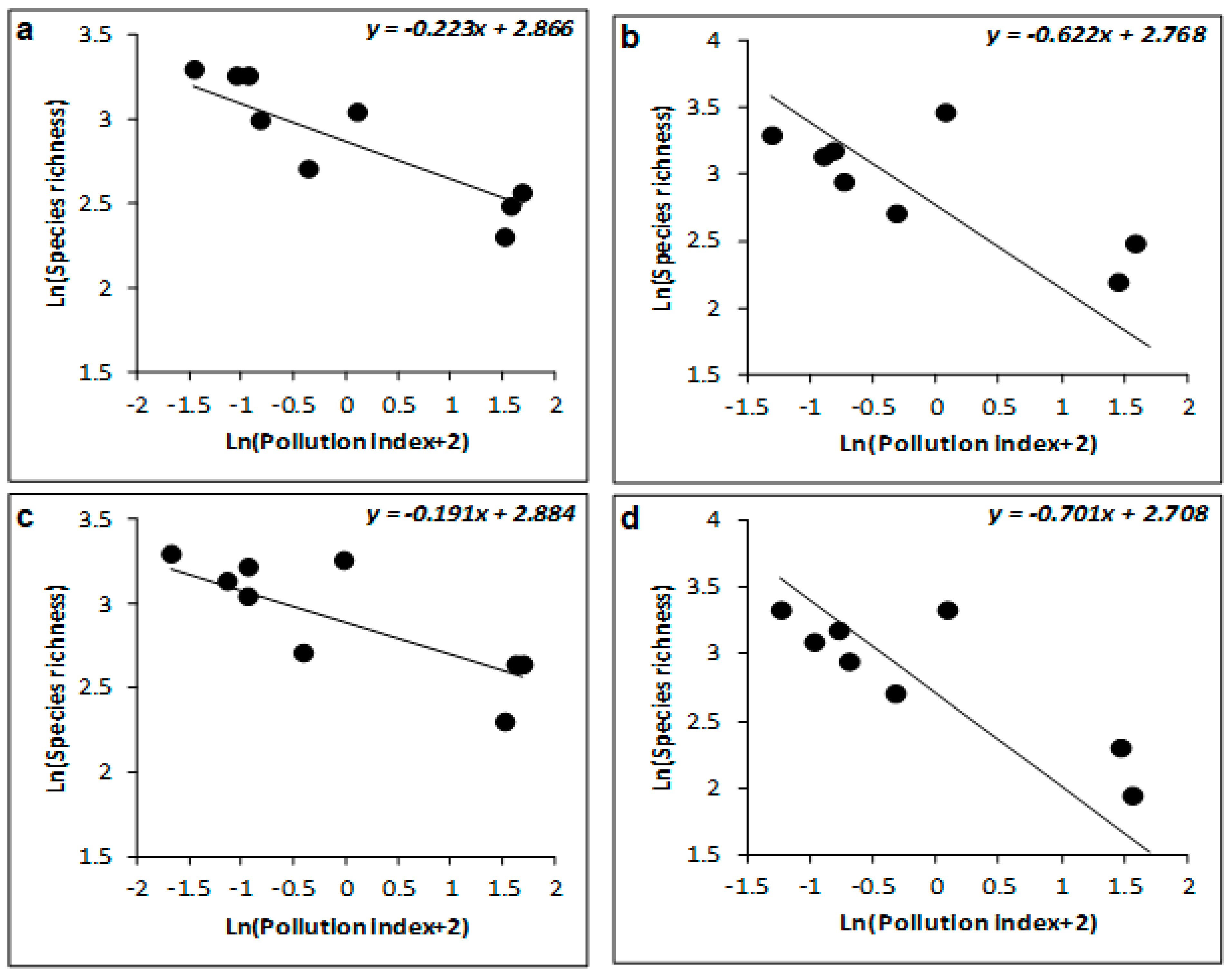
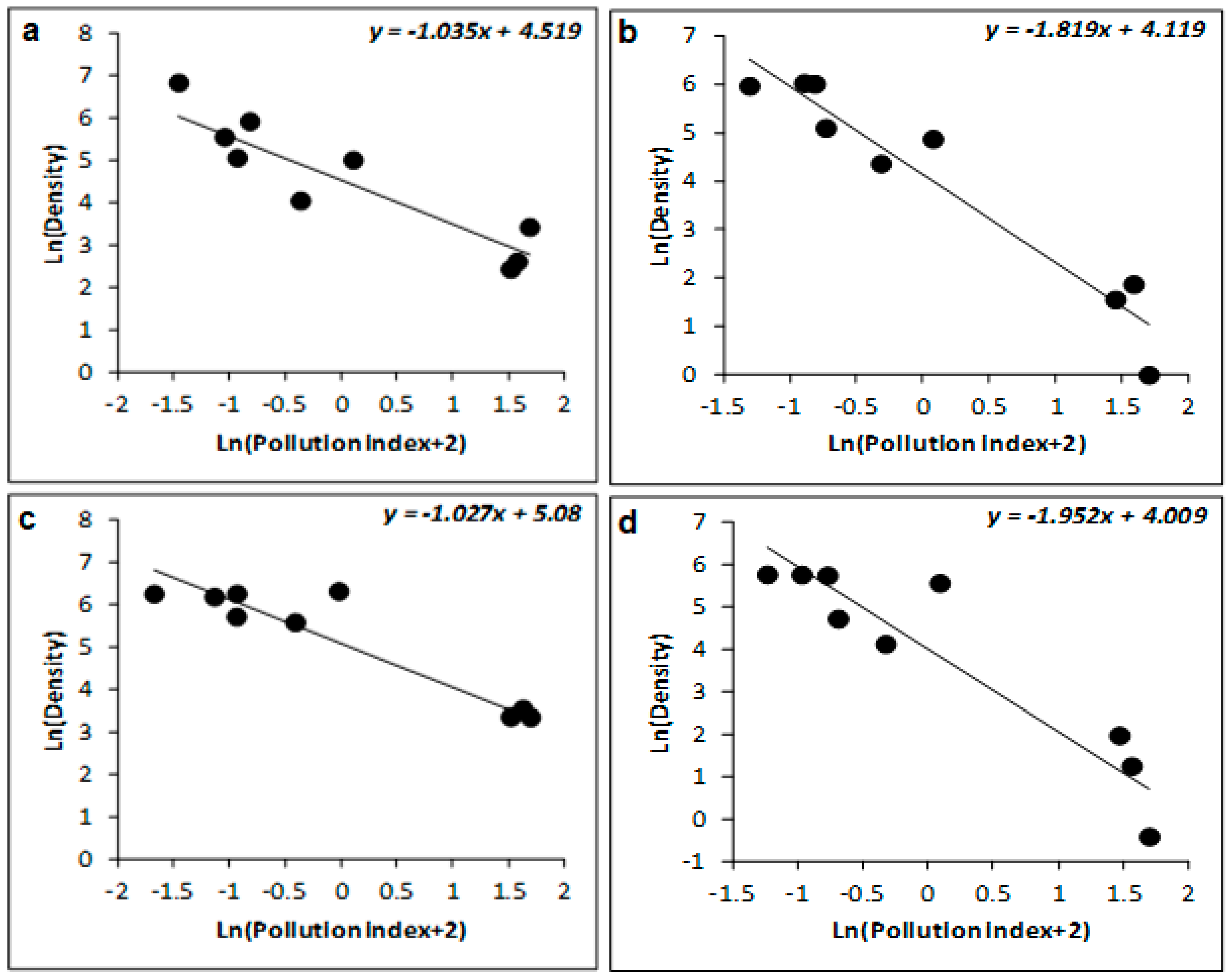
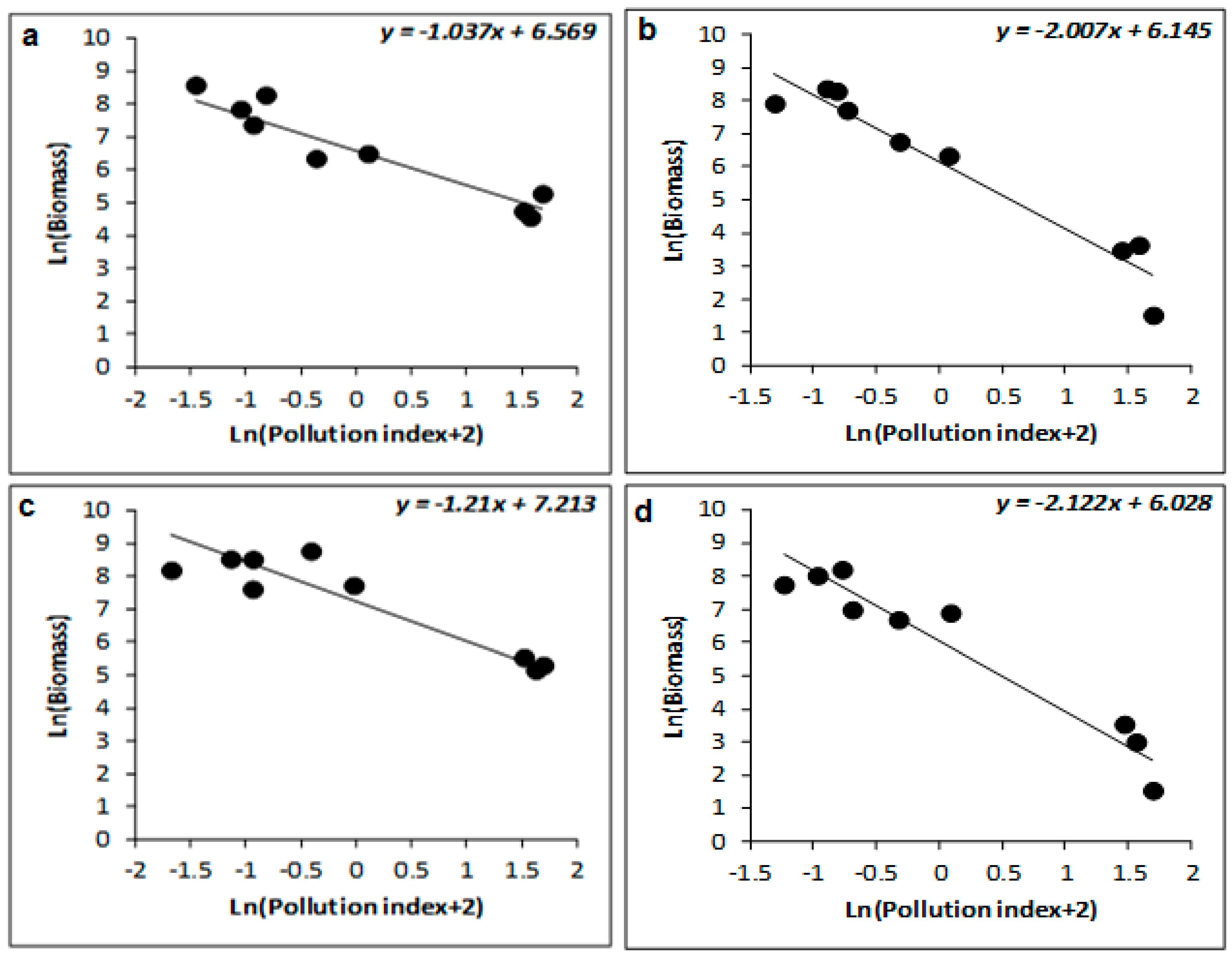
| Winter | 77 | −0.223 ± 0.052 | −4.306 | 0.005 | 88 | −1.035 ± 0.254 | −4.067 | 0.007 | 93 | −1.037 ± 0.185 | −5.612 | 0.001 |
| Spring | 68 | −0.191 ± 0.063 | −3.033 | 0.023 | 93 | −1.027 ± 0.135 | −7.588 | <0.001 | 95 | −1.047 ± 0.214 | −5.642 | 0.001 |
| Summer | 41 | −0.622 ± 0.283 | −2.199 | 0.07 | 78 | −1.819 ± 0.299 | −6.076 | <0.001 | 91 | −2.007 ± 0.347 | −5.782 | 0.001 |
| Autumn | 43 | −0.701 ± 0.231 | −3.039 | 0.023 | 61 | −1.952 ± 0.355 | −5.496 | 0.002 | 78 | −2.122 ± 0.307 | −6.911 | <0.001 |
| Carbohydrates | Study Area | References |
|---|---|---|
| 5–3000 μg·g−1 | North Atlantic coastal zone | [123] |
| 0.67–32.5 μg·g−1 | Ebro Delta (Western Mediterranean) | [124] |
| 6.5–348.9 mg·g−1 | Rhone Delta | [125] |
| 20.3–1356.3 μg·g−1 | coasts of Alexandria (south-eastern Mediterranean) | [126] |
| average 495.7 mg·g−1 | coasts of the city of Barcelona | [127] |
| 10–153 μg·g−1 | Black Sea | [128] |
| 562 à 5697 ng·g−1 | coasts of Crete | [129] |
| Gulf of Gabès | ||
| 1121–5217 mg·kg−1 | Coastal area of the city of Sfax | [121] |
| 928–5108 mg·kg−1 | Coastal area of the city of Sfax | [122] |
| 21–4379.06 μg·g−1 | Coastal area of the city of Gabès | current study |
| LTEL | Gulf of Gabès (Current Work) | |
|---|---|---|
| Fe | 18.84% | 23.19% (S8)–646.38% (S4) |
| Cd | 0.583 mg/kg | 287 (S2)–512 (S3) mg/kg |
| Zn | 98 mg/kg | 64 (S9)–3473 (S3) mg/kg |
| Cu | 28.012 mg/kg | 7.87 (S3)–139.02 (S1) mg/kg |
| F | 6.97 ± 1.07 mg/g | 0 (S6)–5.81 (S2) g/kg |
| Biotope | Copepod’s Densities (ind./10 cm²) | References |
|---|---|---|
| Bay of Arcachon, France | 13–1660 | [158] |
| Tunis lagoon before sanitation | 3–136 | [159] |
| Marenne, France | 139–3088 | [160] |
| Island of Tudy, France | 51–988 | [161] |
| Bayou (Louisiana), USA | 6–146 | [162] |
| Hunter river, Australia | 0–71 | [163] |
| Cap York, Australia | 0–57 | [164] |
| Bizerte Lagoon | 19–132 | [84] |
| Bay of Bizerte | 1–92 | [85] |
| Lagune Sud de Vase noire Tunis | 8–107 | [165] |
| Tunis Lagoon after sanitation | 70–260 | [166] |
| Ghar El Melh Lagoon | 0–77 | [88] |
| Bou Ghrara Lagoon | 0–256 | [88] |
| Libanes coasts | 0–974 | [167] |
| Gulf of Gabès | 0.66 ± 1.15– 929.75 ± 112.84 | current study |
Publisher’s Note: MDPI stays neutral with regard to jurisdictional claims in published maps and institutional affiliations. |
© 2022 by the authors. Licensee MDPI, Basel, Switzerland. This article is an open access article distributed under the terms and conditions of the Creative Commons Attribution (CC BY) license (https://creativecommons.org/licenses/by/4.0/).
Share and Cite
Amorri, J.; Veit-Köhler, G.; Boufahja, F.; Abd-Elkader, O.H.; Plavan, G.; Mahmoudi, E.; Aïssa, P. Assessing Metallic Pollution Using Taxonomic Diversity of Offshore Meiobenthic Copepods. Sustainability 2022, 14, 15670. https://doi.org/10.3390/su142315670
Amorri J, Veit-Köhler G, Boufahja F, Abd-Elkader OH, Plavan G, Mahmoudi E, Aïssa P. Assessing Metallic Pollution Using Taxonomic Diversity of Offshore Meiobenthic Copepods. Sustainability. 2022; 14(23):15670. https://doi.org/10.3390/su142315670
Chicago/Turabian StyleAmorri, Jalila, Gritta Veit-Köhler, Fehmi Boufahja, Omar H. Abd-Elkader, Gabriel Plavan, Ezzeddine Mahmoudi, and Patricia Aïssa. 2022. "Assessing Metallic Pollution Using Taxonomic Diversity of Offshore Meiobenthic Copepods" Sustainability 14, no. 23: 15670. https://doi.org/10.3390/su142315670
APA StyleAmorri, J., Veit-Köhler, G., Boufahja, F., Abd-Elkader, O. H., Plavan, G., Mahmoudi, E., & Aïssa, P. (2022). Assessing Metallic Pollution Using Taxonomic Diversity of Offshore Meiobenthic Copepods. Sustainability, 14(23), 15670. https://doi.org/10.3390/su142315670