Multi-Scale Remaining Useful Life Prediction Using Long Short-Term Memory

Abstract

Predictive maintenance based on performance degradation is a crucial way to reduce maintenance costs and potential failures in modern complex engineering systems. Reliable remaining useful life (RUL) prediction is the main criterion for decision-making in predictive maintenance. Conventional model-based methods and data-driven approaches often fail to achieve an accurate prediction result using a single model for a complex system featuring multiple components and operational conditions, as the degradation pattern is usually nonlinear and time-varying. This paper proposes a novel multi-scale RUL prediction approach adopting the Long Short-Term Memory (LSTM) neural network. In the feature engineering phase, Pearson’s correlation coefficient is applied to extract the representative features, and an operation-based data normalisation approach is presented to deal with the cases where multiple degradation patterns are concealed in the sensor data. Then, a three-stage RUL target function is proposed, which segments the degradation process of the system into the non-degradation stage, the transition stage, and the linear degradation stage. The classification of these three stages is regarded as the small-scale RUL prediction, and it is achieved through processing sensor signals after the feature engineering using a novel LSTM-based binary classification algorithm combined with a correlation method. After that, a specific LSTM-based predictive model is built for the last two stages to produce a large-scale RUL prediction. The proposed approach is validated by comparing it with several state-of-the-art techniques based on the widely used C-MAPSS dataset. A significant improvement is achieved in RUL prediction performance in most subsets. For instance, a 40% reduction is achieved in Root Mean Square Error over the best existing method in subset FD001. Another contribution of the multi-scale RUL prediction approach is that it offers more degree of flexibility of prediction in the maintenance strategy depending on data availability and which degradation stage the system is in.

1. Introduction

Predictive maintenance (PdM) has become the most promising maintenance strategy in Industry 4.0 [1], which can significantly reduce maintenance costs and ensure critical components’ reliability and safety [2]. Remaining useful life (RUL) prediction of engineering components and systems is one of the essential tasks in PdM. RUL prediction generally refers to the study of predicting the specific time length from the current time to the end of the useful life of an asset or system [3]. It is a critical step to minimise catastrophic failures, and it has become an important measurement to achieve the ultimate goal of zero-downtime performance in industrial systems [4].

Approaches for RUL prediction can be catalogued into model-based, data-driven, and hybrid methods. Model-based approaches, also called physics-based approaches, evaluate the health condition of a system by building mathematical models based on the failure mechanisms or the first principle of damage [5,6]. The complex and noisy working conditions often impede the construction of a physical model; cooperating in the model is usually tricky [6]. Meanwhile, it is often difficult to determine the parameters of the physical model. In data-driven approaches, RUL is computed through statistical and probabilistic methods by utilising historical information and routinely monitored data of the system [6]. With the presence of multivariate time sequence signals derived from parallel measurement of hundreds of process variables with various sensors, the application of many machine learning (ML) models for RUL prediction has significantly been promoted [7]. Hybrid approaches, combining model-based and data-driven approaches, aim to leverage the advantages of both categories. Deep learning (DL), a subset of data-driven approaches attracting significant investigations in the last few years in RUL prediction, can extract multilevel features from data [8]. As an end-to-end ML method, DL algorithms can automatically process the original signal, identify discriminative and trend features in the input data layer by layer, and improve generalisation performance [9]. Because of its strength in self-learning features, DL has already achieved great success in the manufacturing industry [10].

An inherent challenge for predicting the RUL of a system is to determine the desired output value for each input data point. Without an accurate physics-based model, it is impossible to accurately identify the system health status at each time step in real-world applications [10]. Generally, there are two solutions to this problem. One is to simply assign the desired output as the actual time left before functional failure, and another is to derive the desired output values based on a suitable degradation model. We would like to discuss this challenge based on NASA’s Commercial Modular Aero-Propulsion System Simulation (C-MAPSS) dataset as one of the most popular multivariate benchmark datasets for evaluating predictive DL algorithms. For C-MAPSS, a piece-wise linear degradation model has been proposed [11]. This model assumes that the degradation of the system typically only begins after a certain degree of usage. The threshold value is determined based on the observations, and its numerical value differs for each dataset. Since then, this model has been adopted by most of the related research.

It should be noted that the threshold value achieved in this paper is 130 based on the first subset (FD001). However, the application of this threshold value has been extended to other subsets (FD00x) in plenty of later research without sufficient justification. Yuan et al. [12] proposed a novel dynamic differential technology that extracts inter-frame information, promoting cognition about the model degradation process. A support vector machine (SVM) is used as an anomaly detector to identify where the system starts degrading, while SVM tends to overfit because the involved kernel and penalty parameters need to be determined [13]. An RUL prediction approach based on degradation pattern learning using a back-propagation neural network [14]. A piece-wise linear distribution function promotes a proportion of the tail samples with a threshold of 120. Ahmed et al. [15] designed a new LSTM architecture that uses the sensor readings to estimate the system’s health, which is then mapped to the target RUL. It is claimed that the proposed method requires no assumptions about the degradation function patterns or the point at which the degradation starts. A Denoising Online Sequential Extreme Learning Machine with Double Dynamic Forgetting Factors (DDFF) and Updated Selection Strategy (USS) is proposed by Berghout et al. [16]. The Online Sequential Extreme Learning Machine (OS-ELM) is used to fit the non-accumulative linear degradation function of the engine to address dynamic programming by tracking the new coming data and gradually forgetting the old ones based on DDFF. The piece-wise linear function is used as the RUL target function, and the threshold is 130. Chen et al. [17] presented a Gated Recurrent Unit (GRU) based neural network that has also been used to extract and learn the nonlinear degradation patterns in the dataset, where the linear function is used as the RUL target function. An unsupervised pre-trained model for turbofan RUL prediction is proposed by Listou Ellefsen et al. [4]. This approach utilised an unsupervised and semi-supervised method to train a model to extract the features and then use the Genetic Algorithm (GA) to determine the threshold value. Shi & Chehade [4] proposed a dual LSTM with changing detection capability. A health index construction function is utilised to help detect change points in sensor measurements and determine the threshold value. A causal augmented convolution network (CaConvNet) has been presented by Ayodeji et al. [7]. The network is further optimised with a dynamic hyperparameter search algorithm to reduce uncertainties and minimise manual selection. A piece-wise linear function and a threshold value of 130 are adopted. Shi and Chehade proposed a dual-LSTM framework [18] that combines change point detection and RUL prediction. They adopted the piece-wise RUL target function but assumed the threshold value to be the midpoint of the degradation process for every engine. Li et al. [19] proposed a GRU-based high-level feature fusion block to replace the traditional fully connected layer and introduced a novel activation function Mish to perform the RUL prediction of aero-engine. They also used the piece-wise linear function, with a fixed threshold of 120 for all four subsets [20]. Zhang et al. [21] used the piece-wise linear function with a novel approach to identify the threshold [19]. The thresholds for all engines are different and determined using a health status assessment evaluated by a bidirectional gated recurrent unit (BiGRU) and multi-gate mixture-of-experts (MMoE).

It should be noted that most of the previous research adopted a nonlinear RUL target function except in which the degradation process of the system is assumed to be linear with usage [16]. The widely used piece-wise linear RUL target function with a fixing threshold of 130 accepts the degradation process of a system transitions directly from a plateau to a linear decline, and the yielding point is located at the RUL of 130. In a real-life application, once the yielding point is reached, the system’s degradation speed will accelerate until the failure occurs. The maintenance strategy should be based on the degradation rate. Most of the solutions are to predict the RUL directly using the whole past data. However, the prediction accuracy varies from engine to engine due to the inconsistent volumes of data collected from different engines and different initial conditions. Therefore, the prediction performance can be unreliable for some engines.

This paper proposes a multi-scale RUL prediction solution using LSTM with a novel RUL target function. The new RUL target function includes a transition stage between the non-degradation and linear degradation stages, aiming to better represent the engine system’s degradation process. The multi-scale prediction solution consists of a small-scale RUL prediction, where the system’s condition is classified into these three stages, and a large-scale RUL prediction, which refers to the prediction of the RUL value for the last two stages. Besides the higher RUL prediction accuracy, the proposed approach also aims to provide more flexibility in the maintenance strategy with this multi-scale RUL prediction solution. For instance, based on the small-scale RUL prediction, maintenance can be arranged when the engine system steps into the linear degradation stage. Or, based on the large-scale RUL prediction, maintenance can be arranged when the prediction value is lower than a certain threshold.

Four main contributions are presented in this paper in order to predict the RUL:

(1)

Extracting the valuable features by using Pearson’s correlation coefficient. Pearson’s correlation coefficient is used to find the correlation between the signals from sensors and the output RUL, as well as the correlation between the signals from sensors.

(2)

Adopting the operation-based normalisation approach. An operation-based normalisation is proposed for the engine system working under multiple operation conditions to reveal the actual degradation patterns concealed in the sensor data.

(3)

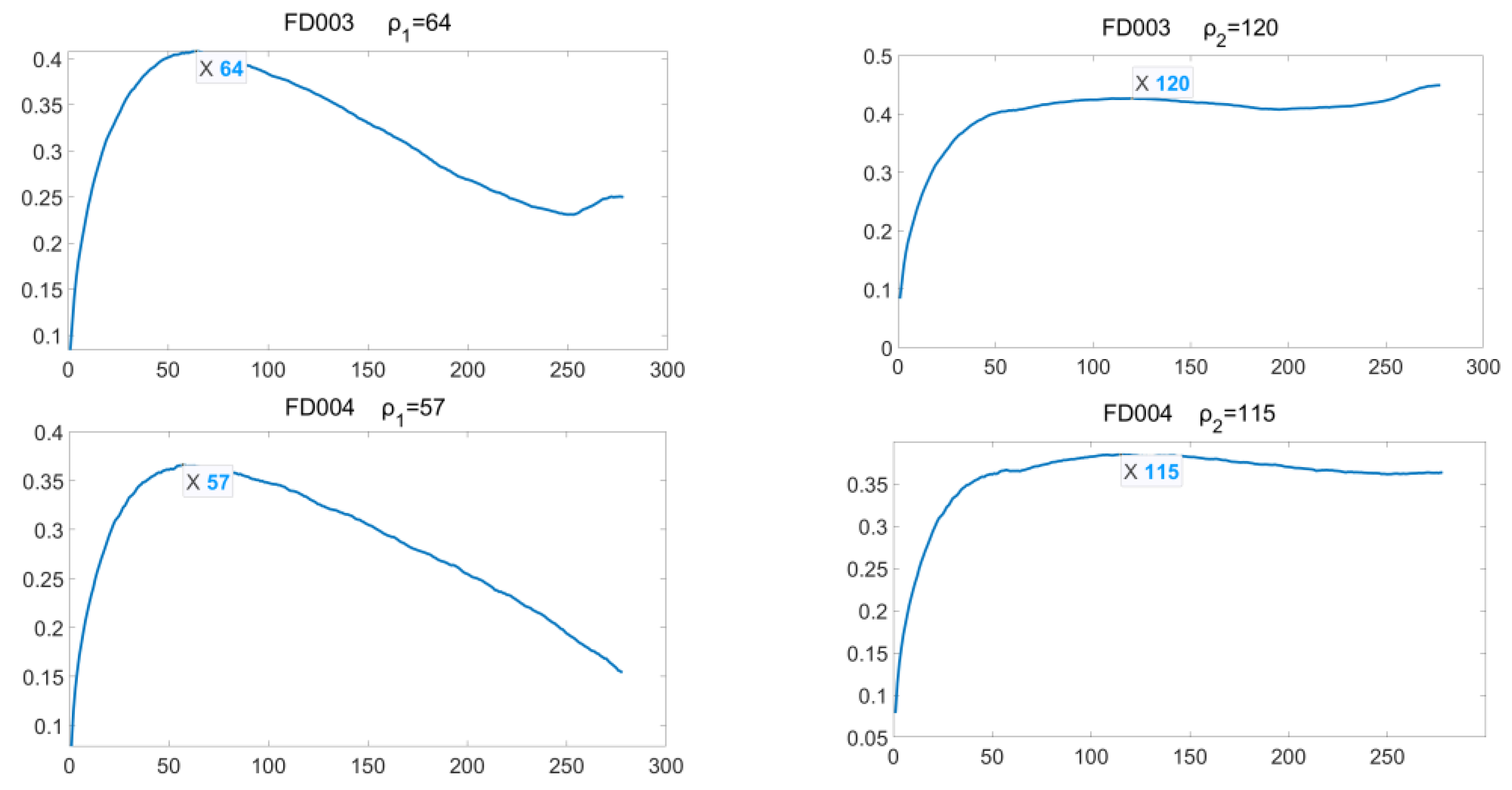
Proposing a new RUL target function for the training process. To define an approximation of the actual RUL, we assume the degradation process of the engine system goes through a constant stage, a transition stage and a linear degradation stage. The turning points of these three stages differ from engine to engine because of the different initial, operating and fault conditions. This paper proposes a correlation-based method to detect these turning points.

(4)

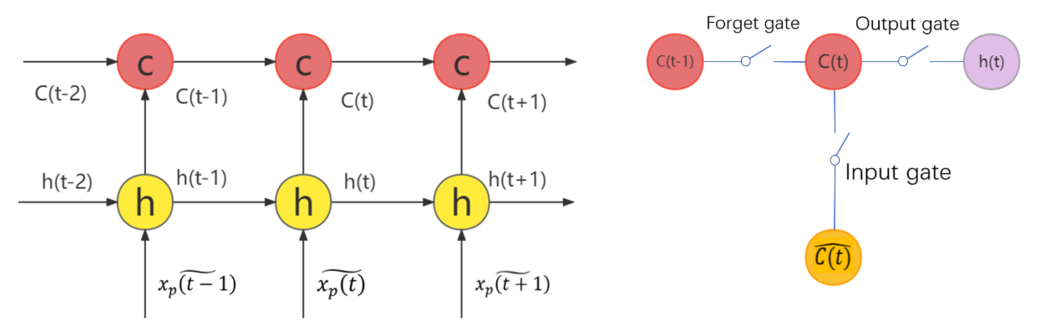
Proposing a multi-scale RUL prediction solution using LSTM. An LSTM-based classification model is used to sort each input data point into the three stages defined in the new RUL target function as the small-scale RUL prediction. Then, the data in the transition and linear degradation stage is fed into another LSTM-based regression model to achieve the large-scale RUL prediction.

The paper is structured as follows: Section 2 describes the C-MAPSS datasets. Section 3 introduces the proposed multi-scale RUL prediction approach. Section 4 reports the performance of the proposed method and the comparison with the state-of-the-art techniques for RUL prediction, and the conclusion is given in Section 5.

2. Dataset Description

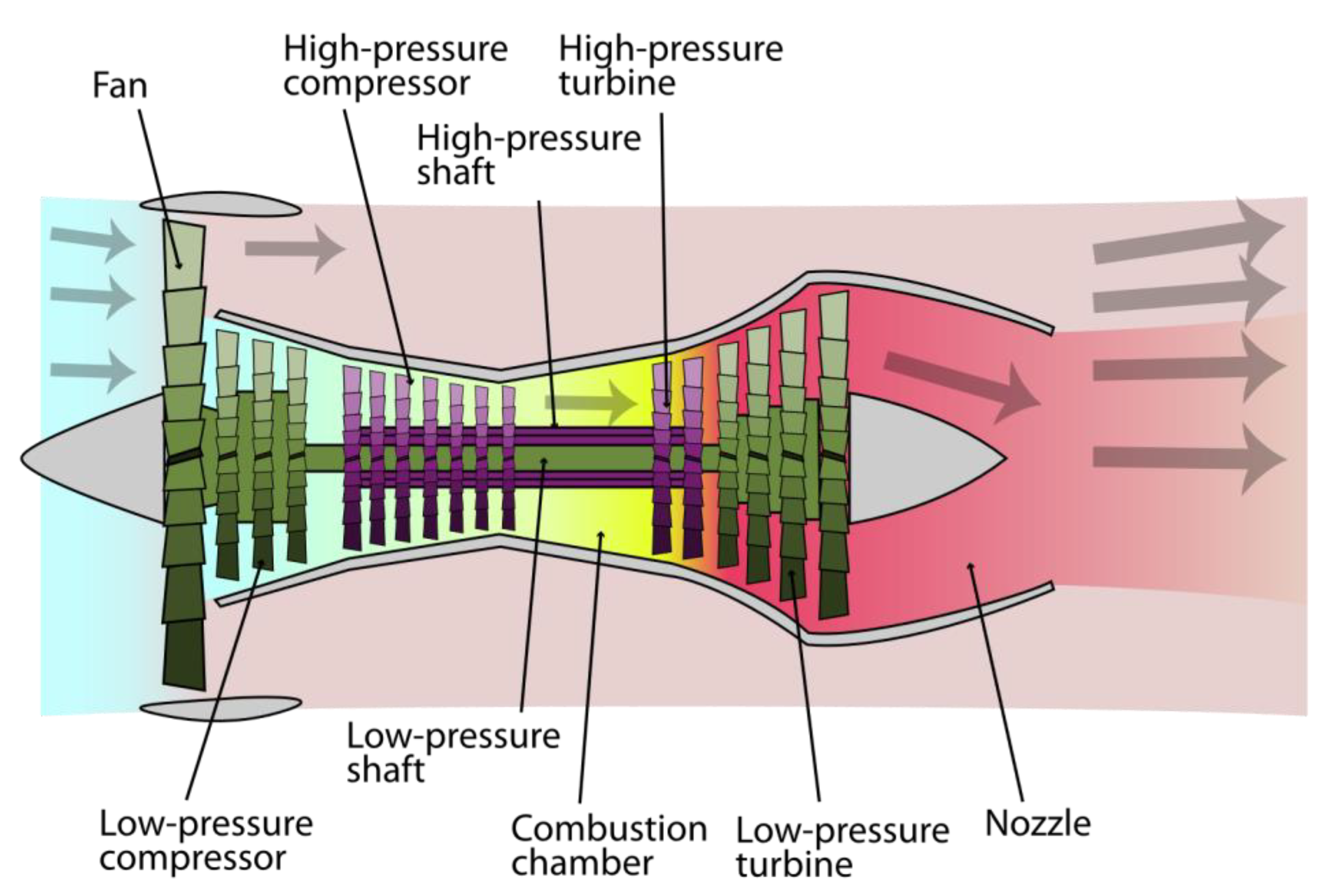
NASA’s C-MAPSS project is a high-fidelity computer model that models the damage propagation of aircraft gas turbine engines [18]. Figure 1 shows the diagram of the simulated run-to-failure trajectories of a small fleet of turbofan engines with the main elements. The simulated engine is a tow spool turbofan engine with a high level of thrust of up to 400,340 N, which operates under operating conditions ranging from sea level to 12,192 (m) of altitude and ambient temperature varying from −51 to 39 °C [22]. The air is introduced into the low-pressure compressor (LPC) through the fan at first in this type of engine. Then, it travels through the high-pressure compressor (HPC) and is heated in the combustor. In the combustor, the compressed air is mixed with fuel and ignited. The fuel combustion provides enough thrust to drive both low-pressure turbines (LPT) and high-pressure turbines (HPT) [16]. A more in-depth explanation can be found in the C-MAPSS User’s Guide [23].

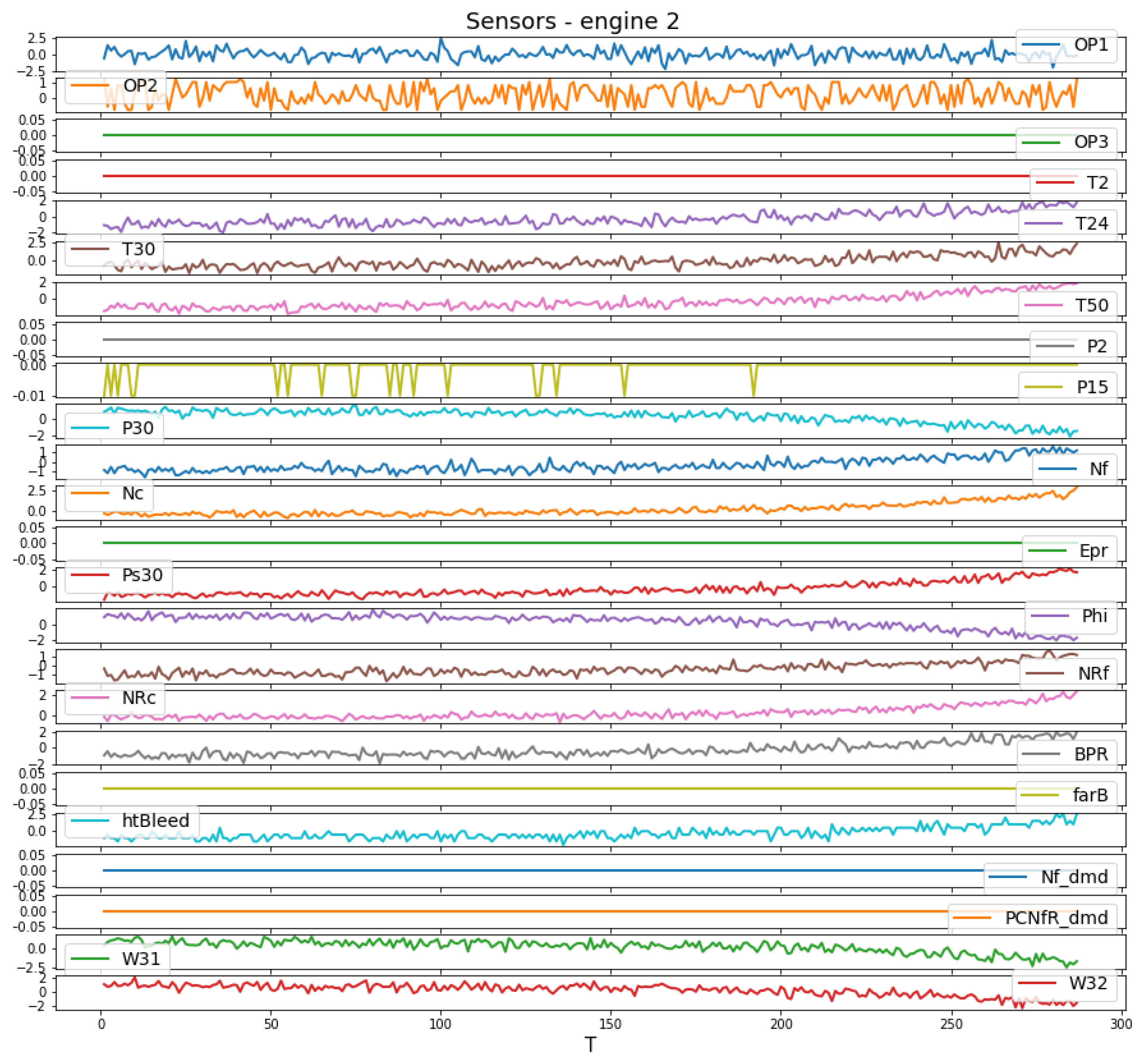
Retrieved data from C-MAPSS software is provided for the public as a benchmark for research on RUL prediction for aircraft engines [18]. The dataset consists of 4 subsets, and each subset has different numbers of engines with varied operational cycles. In this dataset, engine profiles were simulated with different initial degradation conditions. The maintenance was not considered during the simulation. The dataset includes one training set and one testing set for each engine, which contains a multivariate time series of 26 features (engine number, time cycles, three operating condition measurements and 21 sensor measurements). The objective is to predict the RUL of each engine based on the given sensor measurements. The information on the four subsets is listed in

Table 1. C-MAPSS dataset.

Dataset	FD001	FD002	FD003	FD004
Number of engines for training	100	260	100	249
Number of engines for testing	100	259	100	248
Operating conditions	single	multiple	single	multiple
Fault conditions	compressor	compressor	compressor & fan	compressor & fan

. Specifically, FD001 refers to the engine failure arising from the high-pressure compressor under a single operating condition. FD002 refers to the engine failure from the high-pressure compressor under six operation conditions. FD003 refers to the engine failure from the high-pressure compressor and the fan under a single operating condition. FD004 refers to the engine failure from the high-pressure compressor and the fan under six operation conditions. In this study, FD001 was primarily used to demonstrate the proposed solution because the data volume is relatively small to achieve time efficiency. The other three datasets were also tested to validate this method.

The employed dataset comprises information relating to 100 different turbines with a total number of observations varying from 128 to 362. The descriptive statistics of the response and the predictor variables are summarised in

Table 2. Descriptive statistics of all the variables of dataset FD001.

Index	Symbol	Input Variables	Mean	Standard Deviation
1	ID	Engine ID
2	T	Time cycle	108.81	68.88
3	OP1	Operation condition 1	−8.9 × 10−6	0.003
4	OP2	Operation condition 2	2.4 × 10−6	0.003
5	OP3	Operation condition 3	100.00	10−6
6	T2	Total temperature at fan inlet (°R)	518.67	0
7	T24	Total temperature at LPC outlet (°R)	642.68	0.5
8	T30	Total temperature at HPC outlet (°R)	1590.52	6.1
9	T50	Total temperature at LPT outlet (°R)	1408.93	9
10	P2	Pressure at fan inlet (psia)	14.62	3.39 × 10−6
11	P15	Total pressure in bypass-duct (psia)	21.61	0.001
12	P30	Total pressure at HPC outlet (psia)	553.37	0.89
13	Nf	Physical fan speed (rpm)	2388.10	0.07
14	Nc	Physical core speed (rpm)	9065.24	22.08
15	Epr	Engine pressure ratio (P50/P2)	1.30	4.66 × 10−13
16	Ps30	Static pressure at HPC outlet (psia)	47.54	0.27
17	Phi	Ratio of fuel flow to Ps30 (pps/psi)	521.41	0.74
18	NRf	Corrected fan speed (rpm)	2388.10	0.72
19	NRc	Corrected core speed (rpm)	8143.75	19.08
20	BPR	Bypass ratio	8.44	0.04
21	farB	Burner fuel–air ratio	0.03	1.56 × 10−14
22	htBleed	Bleed enthalpy	393.21	1.55
23	Nf_dmd	Demanded fan speed (rpm)	2388.00	0
24	PCNfR_dmd	Demanded corrected fan speed (rpm)	100.00	0
25	W31	HPT coolant bleed (lbm/s)	38.82	0.18
26	W32	LPT coolant bleed (lbm/s)	23.28	0.11

. The location of each sensor is illustrated in Figure 2.

Since Root Mean Square Error (RMSE) is the most widely used indicator in residual life prediction [24]. It was used to evaluate the performance of the trained neural networks in this case study. The mathematical expression is:

$$\mathrm{RMSE}=\sqrt{\frac{1}{\mathrm{n}}{\displaystyle \sum }_{\mathrm{i}=1}^{\mathrm{n}}{\left({\widehat{y}}_i-y_i\right)}^2 }$$

(1)

where $\mathrm{n}$ is the total number of actual RUL targets in the related testing dataset and $y_i$ refers to the true RUL and ${\widehat{y}}_i$ refers to the predicted RUL at the time cycle i.

3. Methodology

The proposed scheme of multi-scale RUL prediction is shown in Figure 3b. At first, the feature selection method is used to refine the number of input variables to reduce the computational cost of modelling and improve the model’s prediction performance by reducing interference from noise. Then, a proposed operation condition-based stabilisation technique is applied to the selected variables to stabilise the model’s training dynamics. After that, based on the assumption that the degradation process of the system includes three stages, a correlation-based method is proposed to estimate the two thresholds that can divide the original training set into three parts. An LSTM-based 3-stage classification model is then established to automatically determine the degradation stage for each cycle time based on the selected inputs only, which acts as a small-scale RUL prediction. Finally, another LSTM-based model for the last two stages is performed to predict the large-scale RUL. Each step will be explained in more detail.

3.1. Feature Selection

An accurate prognosis relies on effective feature extraction from the whole series to capture valuable information and discard irrelevant noise [25]. Feature selection primarily focuses on removing non-informative or redundant variables from the data that do not contribute to the model’s prediction accuracy or cause overfitting problems. Since the RUL prediction of a system is a regression predictive modelling problem with numerical input and output variables, Pearson’s correlation coefficient is the most common method to use in this area [20]. Pearson’s correlation coefficient measures the strength of the linear relationship between two data samples. Pearson’s correlation coefficient is widely adopted to extract informative features in the ML field. For example, it is used to remove the highly intercorrelated figures in [26], and the selected features are used to predict the ship’s propulsion power.

In this case, we assume the input variables as ${\mathrm{x}}_{\mathrm{i}}\left(\mathrm{t}\right)$, where $\mathrm{i}=1,2,\dots , 26;\mathrm{t}=1,2,\dots ,\mathrm{n}$; $\mathrm{n}$ is the number of observations, and we assume the output RUL is $\mathrm{y}\left(\mathrm{t}\right)$. We selected the most valuable features through three steps. Take dataset FD001 as an example. The first step is to find the descriptive statistics of all the variables. Based on Table 2, the sensor measurements T2, Nf_dmd and PCNfR_dmd are constant, and the standard deviation of OP3, P2, Epr and farB are almost equal to zero. Therefore, these seven nugatory variables are discarded to reduce the computation cost. The second step is calculating the Pearson correlation between the selected input variable ${\mathrm{x}}_{\mathrm{p}}$ and ${\mathrm{x}}_{\mathrm{q}}$ following formula Equation (2). The last step is to figure out the Pearson correlation between the selected input variable ${\mathrm{x}}_{\mathrm{p}}$ and output $\mathrm{y}$ following Equation (3).

$${\mathrm{r}}_{{\mathrm{x}}_{\mathrm{p}},{\mathrm{x}}_{\mathrm{q}}}=\frac{n{{\displaystyle \sum }}_{t=1}^n{\mathrm{x}}_{\mathrm{p}}\left(\mathrm{t}\right){\mathrm{x}}_{\mathrm{q}}\left(\mathrm{t}\right)-{{\displaystyle \sum }}_{t=1}^n{\mathrm{x}}_{\mathrm{p}}\left(\mathrm{t}\right){{\displaystyle \sum }}_{t=1}^n{\mathrm{x}}_{\mathrm{q}}\left(\mathrm{t}\right)}{\sqrt{n{{\displaystyle \sum }}_{t=1}^n{\mathrm{x}}_{\mathrm{p}}{\left(\mathrm{t}\right)}^2-{\left({{\displaystyle \sum }}_{t=1}^b{\mathrm{x}}_{\mathrm{p}}\left(\mathrm{t}\right)\right)}^2}\sqrt{n{{\displaystyle \sum }}_{t=1}^n{\mathrm{x}}_{\mathrm{q}}{\left(\mathrm{t}\right)}^2-{\left({{\displaystyle \sum }}_{t=1}^n{\mathrm{x}}_{\mathrm{q}}\left(\mathrm{t}\right)\right)}^2}}$$

(2)

$${\mathrm{r}}_{{\mathrm{x}}_{\mathrm{p}},\mathrm{y}}=\frac{n{{\displaystyle \sum }}_{t=1}^n{\mathrm{x}}_{\mathrm{p}}\left(\mathrm{t}\right)\mathrm{y}\left(\mathrm{t}\right)-{{\displaystyle \sum }}_{t=1}^n{\mathrm{x}}_{\mathrm{p}}\left(\mathrm{t}\right){{\displaystyle \sum }}_{t=1}^n\mathrm{y}\left(\mathrm{t}\right)}{\sqrt{n{{\displaystyle \sum }}_{t=1}^n{\mathrm{x}}_{\mathrm{p}}{\left(\mathrm{t}\right)}^2-{\left({{\displaystyle \sum }}_{t=1}^b{\mathrm{x}}_{\mathrm{p}}\left(\mathrm{t}\right)\right)}^2}\sqrt{n{{\displaystyle \sum }}_{t=1}^n\mathrm{y}{\left(\mathrm{t}\right)}^2-{\left({{\displaystyle \sum }}_{t=1}^n\mathrm{y}\left(\mathrm{t}\right)\right)}^2}}$$

(3)

${\mathrm{r}}_{{\mathrm{x}}_{\mathrm{p}}\left(\mathrm{t}\right){ \mathrm{x}}_{\mathrm{q}}\left(\mathrm{t}\right)}$, ${\mathrm{r}}_{{\mathrm{x}}_{\mathrm{p}}\left(\mathrm{t}\right),\mathrm{y}\left(\mathrm{t}\right)}$ are the correlation coefficient between ${\mathrm{x}}_{\mathrm{p}}\left(\mathrm{t}\right)$ and ${\mathrm{x}}_{\mathrm{q}}\left(\mathrm{t}\right)$, ${\mathrm{x}}_{\mathrm{p}}\left(\mathrm{t}\right)$ and $\mathrm{y}\left(\mathrm{t}\right)$, range from −1 to +1. A correlation coefficient of 1 indicates that for every positive increase in one variable, there is a positive increase of fixed proportion in another variable. A correlation coefficient of -1 means that for every positive increase in one variable, there is a negative decrease of fixed proportion in another variable. A correlation coefficient of 0 means that these two variables are unrelated. The absolute value of the correlation coefficient refers to the relationship strength between the two variables. The selection of the thresholds will affect the volume of the dataset that feeds into the model and then affect the prediction performance. Therefore, we only discarded the highly correlated variables. In this case, one of the two variables will be discarded if ${\mathrm{r}}_{{\mathrm{x}}_{\mathrm{p}}\left(\mathrm{t}\right),{\mathrm{x}}_{\mathrm{q}}\left(\mathrm{t}\right)}$ is higher than 0.95. We have tested different thresholds, and it has been found that the value of 0.95 achieves the best result for this dataset. Similarly, we only discarded the extremely irrelevant variables: in other words, when ${\mathrm{r}}_{{\mathrm{x}}_{\mathrm{p}}\left(\mathrm{t}\right),\mathrm{y}\left(\mathrm{t}\right)}$ is extremely close to zero. Based on many tests, the threshold is set to 0.01.

3.2. Data Normalisation

Normalisation techniques are generally necessary to train deep neural networks [24]. The beneficial properties of this technique include the ability to propagate informative activation patterns in deeper layers, reduced dependence on initialisation, smoothing of loss landscape and so on. In this case, we applied the MinMaxScaler to rescale the data from the original range to a new fixed range between 0 and 1. This scaler assumes that the data’s minimum and maximum observable values are provided or can be accurately estimated. For the selected input $x_p\left(t\right)$, the transformation equation is given by:

$$\widetilde{x_p}\left(t\right)=\frac{x_p\left(t\right)-\min (x_p\left(t\right))}{\max (x_p\left(t\right))-\min \left(x_p\left(t\right)\right)}$$

(4)

To address the cases where multiple degradation patterns are concealed in the sensor data, such as datasets FD002 and FD004, we propose an operation-based data scaling. The concept is to scale the data under the same operation condition and then reconstruct them back to their original order. In this way, the influence of different operating conditions can be minimised. We first utilise the unsupervised k-Means clustering based on the selected input variables to classify all raw input variables $x_p\left(t\right)$ in terms of different operational conditions ($O{C}_1$, $O{C}_2,\dots ,O{C}_N$). Then each input variable $\widehat{x_p}\left(t\right)$ is reconstructed by connecting with all normalised segments with the same time index shown in Equation (5), written as

$$\widehat{x_p}\left(t\right)={\displaystyle \bigcup }_{j=1}^N\mathrm{Norm}\left|x_p\left(t\left(O{C}_j\right)\right)\right|$$

(5)

where N is the number of operational conditions and $\mathrm{Norm}\left|·\right|$ denotes the MinMax normalisation operation.

3.3. RUL Target Function

Accurately determining the system health status at each time step is an inherent challenge for data-driven prognostic problems. One sensible solution is to simply assign the desired output as the time left before the occurrence of the failure, which indicates that the system’s health degrades linearly with usage. The advantage of this solution is that it strictly follows the RUL definition, which is defined as the time to failure. The linear model is the most natural option when the degradation model is unknown, as shown in Figure 4a. Another approach is applying a suitable degradation model for this dataset, specifically the piece-wise linear degradation model. The RUL is assumed to be constant until it crosses a certain threshold which can be seen [14] in Figure 4b. This approach is more reasonable because the degradation of the system usually starts after a certain degree of usage. Also, it is more likely to prevent the model from overestimating the RUL. The reason is that the data used to train the network is from run-to-failure samples, and the samples in the testing dataset are still within the service life. The prediction error will be substantial for the engines still in the initial usage stage.

Similar to the piece-wise linear degradation model, this study assumes that the degradation of the system only starts after a certain degree of usage. However, this paper also considers that it will not turn into the linear degradation mode directly after the threshold value. Instead, the degradation speed should be slow and then increase over time. Therefore, we propose a three-stage RUL target function, as illuminated in Figure 4c, which includes the constant stage, the transition stage, where the system degrades nonlinearly with usage, and the linear degradation stage.

One challenge for the proposed three-stage degradation process is to find out the two thresholds that can distinguish the whole dataset into three parts. A two-step correlation-based method is introduced to accomplish this work. First, we assume that the RUL degradation is linear temporally, so the RUL can be labelled for each time cycle. Therefore, the RUL of the first time cycle for each engine is the maximum time cycle of that engine. The first threshold ${\rho }_1$ can be calculated by the following equations:

$${\rho }_1=\underset{\tau }{argmax}\frac{1}{m}{\displaystyle \sum }_{p=1}^m\left|r_{\widehat{x_p},\widehat{y_{\tau }}}\right|, \tau =1,2,\dots ,\mathrm{n}$$

(6)

$$\widehat{y_{\tau }}\left(t\right)=\{\begin{array}{c}0, y\left(t\right)>\tau \\ 3,y\left(t\right)\le \tau \end{array}$$

(7)

where $m$ is the number of the selected input variables, and the range of $\tau$ is selected, referring to the average observation numbers of 100 engines. The second threshold ${\rho }_2$ is then computed by

$${\rho }_2=\underset{\tau }{argmax}\frac{1}{m}{\displaystyle \sum }_{p=1}^m\left|r_{\widehat{x_p},\breve{y_{\tau }}}\right|, \tau ={\rho }_1,{\rho }_1+1,\dots ,\mathrm{n}$$

(8)

$$\check{y_{\tau }}\left(t\right)=\{\begin{array}{cc}1& y\left(t\right)>\tau \\ 2& {\rho }_1<y\left(t\right)\le \\ 3& y\left(t\right)\le {\rho }_1\end{array}\tau$$

(9)

3.4. Multi-Scale RUL Prediction

3.4.1. Two-Step LSTM Model for 3-Stage Classification

AN LSTM network is a modified recurrent neural network (RNN) structure designed for sequence learning [27]. It incorporates the standard recurrent layer along with additional “memory” control gates. LSTM uses storage elements to transfer information from the past output instead of having the output of the RNN cell be a nonlinear function of the weighted sum of the current input and previous output. In other words, instead of using a hidden state $h$ only, LSTM adopts a cell state $C$ to keep the long-term information, as shown in Figure 5. The main concept of LSTM is utilising three gates to control the cell state $C$ (forget gate, input gate and output gate). The forget gate is used to control the information from the previous cell state $C\left(t\right)$ to the current cell state $C\left(t\right)$; the input gate decides how many inputs should be kept in the current cell state $C\left(t\right)$, and the output gate determines the output $h\left(t\right)$ from the current cell state $C\left(t\right).$

The output of LSTM at step $t$ is calculated using the following equations:

$$i\left(t\right)=\mathsf{\sigma }\left(U^i\widetilde{x_p\left(t\right)}+W^{i}h\left(t-1\right)+b_i\right)$$

(10)

$$f\left(t\right)=\mathsf{\sigma }\left(U^f\widetilde{x_p\left(t\right)}+W^{f}h\left(t-1\right)+b_f\right)$$

(11)

$$o\left(t\right)=\mathsf{\sigma }\left(U^o\widetilde{x_p\left(t\right)}+W^{o}h\left(t-1\right)+b_o\right)$$

(12)

$$\widehat{C\left(T\right)}=\tan \mathrm{h}\left(U^{\tilde{c}}\widetilde{x_p\left(t\right)}+W^{\widehat{C}}h\left(t-1\right)+b_{\widehat{C}}\right)$$

(13)

$$C\left(t\right)=C\left(t-1\right)·f\left(t\right)+\widehat{C\left(t\right)}·i\left(t\right)$$

(14)

$$h\left(t\right)=\tan \mathrm{h}\left(C\left(t\right)\right)·o\left(t\right)$$

(15)

where $U$, $W$ and $b$ are the trainable weights and biases, respectively, and$i$, $f$ and $o$ represent the input gate, forget gate, and output gate, respectively. These three gates have the same shape with different parameters $U$ and$W$, which need to be learned from the training process. The candidate state $\widehat{C\left(T\right)}$ cannot be used directly. It must pass through the input gate and then be used to calculate the internal storage$C\left(t\right)$, while $C\left(t\right)$ is not only affected by the hidden state but also by $C\left(t-1\right),$ which is controlled by the forget gate. Based on $C\left(t\right)$, a layer of $\tan \mathrm{h}$ function is applied to the output information$h_t$, which is constrained by the output gate. The gates enable LSTM to fulfil the long-term dependencies in the sequence, and by learning the gate parameters, the network can find the appropriate internal storage [28].

The proposed two-step binary classification model is demonstrated in Figure 3a. To implement this LSTM model, the two threshold values ${\rho }_1$, ${\rho }_2$ are required to label the output for the training set. In the first step, ${\rho }_1$ is used to label the data, written as

$$y_1\left(t\right)=\{\begin{array}{c} 3, y\left(t\right)\le {\rho }_1\\ 0, y\left(t\right)>{\rho }_1 \end{array}$$

(16)

Then $y_1\left(t\right)$ and $\widetilde{x_p\left(t\right)}$ (or $\widehat{x_p\left(t\right)}$) are used to train the first model. In the second step, ${\rho }_1$ and ${\rho }_2$ are used to label the data, written as

$$y_2\left(t\right)=\{\begin{array}{c} 2, {\rho }_1<y\left(t\right)\le {\rho }_2\\ 1, y\left(t\right)>{\rho }_2 \end{array}$$

(17)

The data in the stage where $y\left(t\right)\le {\rho }_1$ is neglected in this step. Then $y_2\left(t\right)$ and $\widetilde{x_p}\left(t\right)$ (or $\widehat{x_p}\left(t\right)$) are used to train the second model. Based on these two models, the testing data can be classified into three stages purely based on the input variables $\widetilde{x_p}\left(t\right)$. It should be noted that the original training set is split into two parts: the first 80% of engines for training and the last 20% of engines for validation. The parameters used in the structure include activation function: sigmoid; neuron number: 128; optimiser: Adam; loss function: the binary cross-entropy. It should be noted that the selection of these parameters can impact the accuracy of RUL prediction. The selected parameters in this study are based on a previously detailed investigation of the effect of parametric uncertainty conducted by Wang et al. [28].

3.4.2. LSTM-Based Large-Scale RUL Prediction

Once the engine enters stage 2, the degradation rate is accelerated. A larger scale RUL prediction is then demanded to monitor system performance closely. The data in stage 2 and stage 3 is extracted before feeding selected variables into the LSTM model. The cycle time threshold $t_1$ is determined when

$$y\left(t_1\right)={\rho }_1$$

(18)

The dataset $y\left(t\right)$ and $\widetilde{x_p}\left(t\right)$, where $t=t_1,t_1+1,\dots ,n$, are then used to train the model.

As the volume of the data has been reduced, the validation split is set to be 5% of the original dataset. The parameters used in the structure include the activation function: ReLU, optimiser: Adam, and the loss function: Root Mean Square Error.

4. Results

4.1. Feature Selection

Figure 6 plots the raw sensor measurements of Engine 2 in the dataset FD001, where the variation of each sensor can be observed. Seven sensors (OP3, T2, P2, P15, farB, Nf_dmd, and PCNfR_dmd) have no variation and were discarded in the first step.

The correlation method was then applied to find out the correlation between each selected input variable and the output RUL using Equation (3). Based on the result displayed in

Table 3. Correlation values between each input and the output RUL for Engine 2 in the dataset FD001, where the discarded sensors are highlighted.

Sensor	Correlation Value	Sensor	Correlation Value
Ps30	0.727	T30	0.616
T50	0.711	NRf	0.573
Phi	0.701	Nf	0.571
P30	0.685	Nc	0.448
BPR	0.673	NRc	0.362
W32	0.666	P15	0.121
W31	0.663	OP2	0.010
htBleed	0.640	OP1	0.008
T24	0.632

, the measurements of OP1 and OP2 are dropped because their correlation values are smaller than a pre-set threshold of 0.01.

In the third step, the pairwise correlation coefficients among the selected sensors were calculated using Equation (2), and the results are illustrated in Figure 7. A pre-set threshold of 0.95 was used in this case study. It can be observed that Nc and NRc are highly correlated (r = 0.98), which suggests there is no additional benefit to including both measures for the RUL prediction. Therefore, we dropped the sensor Nc for the following analysis in this study. Through these three steps, the 14 sensors of T24, T30, T50, P15, P30, Nf, Ps30, Phi, NRf, NRc, BPR, htBleed, W31 and W32 are finally selected as the features for the multi-stage RUL prediction in the dataset FD001. The selection of the features can be verified by the practical meaning shown in Table 2. For instance, Nf_dmd and PCNfR_dmd refer to the demanded fan speed and the demanded corrected fan speed. They are fixed values and are not supposed to influence the RUL prediction. In addition, Nc and NRc are physical core speed and corrected core speed, which are supposed to have high intercorrelation.

The feature selection process and the outcome for the datasets FD002–FD004 can be seen in

Table 4. The feature selection process for the datasets FD002–FD004.

Features	FD001	FD002	FD003	FD004
OP1	X(IR)	X(IR)	X(IR)	X(IR)
OP2	X(IR)	X(IR)	X(IR)	X(IR)
OP3	X(CO)	X(CO)	X(CO)	X(CO)
T2	X(CO)	X(CO)	X(CO)	X(CO)
T24	√	√	√	√
T30	√	√	√	√
T50	√	√	√	√
P2	X(CO)	X(CO)	X(CO)	X(CO)
P15	X(CO)	√	√	X(IR)
P30	√	√	X(RE)	X(RE)
Nf	√	X(RE)	X(RE)	X(RE)
Nc	X(RE)	X(RE)	X(RE)	X(RE)
Epr	√	√	√	√
Ps30	√	√	√	√
Phi	√	√	√	√
NRf	√	√	√	√
NRc	√	√	√	√
BPR	√	√	√	√
farB	X(CO)	√	X(CO)	√
htBleed	√	√	√	√
Nf_dmd	X(CO)	X(CO)	X(CO)	X(CO)
PCNfR_dmd	X(CO)	X(CO)	X(CO)	X(CO)
W31	√	√	√	√
W32	√	√	√	√

X = Feature dropped √ = Feature selected IR = Irelavant CO = Constant RE = Redundant.

.

4.2. LSTM Model for 3-Stage Classification

To achieve the 3-stage classification, the two thresholds ${\rho }_1$ and ${\rho }_2$ need to be determined after the MinMax normalisation. Figure 8 plots the mean correlation value against different $\tau$ for the four datasets using Equation (6) (the left column of Figure 8) and Equation (8) (the right column of Figure 8). The $\tau$ values of the peaks are selected as ${\rho }_1$ and ${\rho }_2$. It is observed that ${\rho }_1$ can be easily set with a clear peak, which suggests that the linear degradation stage (the third stage) is relatively easy to be distinguished. The value of ${\rho }_1$ is between 50 to 65 for these datasets. The selection of ${\rho }_2$ is tricky as the mean correlation value doesn’t drop dramatically with large $\tau$ values indicating that the boundary between the transition stage (the second stage) and the constant stage (the first stage) is usually vague. The selection of ${\rho }_2$ in datasets FD001 and FD002 are relatively smaller than those in FD003 and FD004, suggesting that the engines with more fault conditions may enter stage 2 sooner.

After the determination of ${\rho }_1$ and ${\rho }_2$, a two-step LSTM model for the 3-stage classification is established. In the first step, we labelled the normalised data based on Equation (7) and fed it into the LSTM-based binary classification model. In the second step, we labelled the data based on Equation (9) and then discarded the data $\check{y_{\tau }}\left(t\right)=3$. The rest of the data were then fed to another binary classification model. Both models’ classification results are displayed in

Table 5. Results of the binary classification of datasets FD001-FD004.

Dataset	$\mathbf{Threshold} ({\mathit{\rho }}_1/{\mathit{\rho }}_2)$	$\mathbf{Accuracy} ({\mathit{\rho }}_1/{\mathit{\rho }}_2)$
		Train Set	Test Set
FD001	50/90	0.94/0.85	0.96/0.86
FD002	50/75	0.93/0.88	0.92/0.87
FD003	64/120	0.92/0.84	0.95/0.81
FD004	57/115	0.93/0.85	0.88/0.74

, where the model has been run three times, and the average values are recorded. It can be observed that stages 2 and 3 can be distinguished with high accuracy (0.96, 0.92, 0.95 and 0.88 for FD001, FD002, FD003 and FD004, respectively). The accuracy in distinguishing stages 1 and 2 is relatively low (0.86, 0.87, 0.81 and 0.74, respectively). The reason for the prediction difference for different stages is that the degradation process is relatively slow in the initial phase. As seen in Figure 6, the increase or decrease trend in the sensor observation is inconspicuous at the beginning. In addition, that life span is relatively long compared to the engines’ total lifetime, making it harder for the model to learn the features to distinguish stages 1 and 2. Another reason is the selection of ${\mathit{\rho }}_{\mathbf{2}}$ using the correlation-based method is not as precise as the method for determining ${\mathit{\rho }}_{\mathbf{1}}$. FD004, which works under more fault and multiple operational conditions, has the lowest small-scale RUL prediction. Since the operation-based normalisation approach minimised the impact caused by multiple operating conditions, the difference in prediction accuracy mainly results from the fault conditions.

4.3. LSTM-Based RUL Prediction for Stage 2 and Stage 3

In this part, the data in the constant stage ($y\left(t_1\right)\ge {\rho }_2$) is neglected, and only the data in the transition stage (${\rho }_1<y\left(t_1\right)<{\rho }_2$) and the linear degradation stage ($y\left(t_1\right)\le {\rho }_1$) is adopted. These data are then fed to a two-layer LSTM model with labelled RUL. Figure 9 plots the prediction result of the first 20 engines in the training dataset. Generally, the RUL prediction accuracy is relatively poor at the beginning and is in line with the ground truth when close to the failure point, which is in agreement with the result achieved in most literature, such as [1,29]. The most likely reason for this result is that the turning points between the constant and transition stages in different engines in the same dataset are also different. Although these engines suffer from the same operating and fault conditions, the degradation process would not be precisely the same due to other factors like the working environment.

Figure 10 demonstrates the uncertainty quantification of the RUL prediction of all engines in the training set for each subset. It can be observed that the average RUL prediction, indicated by the solid curves, overall aligns with the ground truth. The pink area (indicating the 95% confidence interval) shows the decreasing trend of the uncertainty of RUL prediction following the increment of the lifecycle. The RUL prediction of the first two subsets outperforms that of FD003 and FD004 as they have only one fault condition.

Table 6. RUL prediction performance with different window lengths (wl) for both the train set and the test set (RMSE) (The first 80% of engines in the training set are used for training, and the remaining 20% are used for testing).

Dataset	Training Data Set				Testing Data Set
	wl = 10	wl = 20	wl = 30	wl = 40	wl = 10	wl = 20	wl = 30	wl = 40
FD001	9.15	6.88	5.03	4.21	14.16	9.41	5.95	5.21
FD002	8.71	7.4	6.85	4.22	16.54	16.13	14.95	11.76
FD003	12.55	10.61	9.66	8.37	17.07	17.29	14.35	11.61
FD004	15.88	13.41	10.5	8.75	25.49	22.49	20.18	18.89

demonstrates the large-scale RUL prediction performance of the LSTM-based model on both the training dataset and testing dataset for FD001–FD004 with different window lengths. The result indicates that when the volume of the dataset is guaranteed, a more extended window size usually leads to a better RUL prediction performance, which agrees with the conclusion drawn by [30]. Therefore, one drawback of the proposed model for the RUL prediction is that it segments the dataset into different stages, reducing the data volume of each stage and thereby restricting the window size options. For instance, in the dataset FD002, the data that can be used for training is limited since the threshold to distinguish stage 1 and stage 2 is relatively small (${\rho }_2=75$). Therefore, to ensure the quality of the training, the window size needs to be relatively small in this case. In addition, the RUL prediction performance on dataset FD001 is generally better than the others. The reason is that the engines in this dataset are working only under one operation condition, and there is only one fault condition which means much less noise is involved when recording the measurements.

Table 7. Results of the RUL prediction performance between the proposed method and the state-of-the-art, where the best prediction of each dataset is highlighted.

Model	FD001	FD002	FD003	FD004
DCNN	12.61	22.36	12.64	23.31
DCGAN	10.71	19.49	11.48	19.71
RBM + LSTM [4]	12.56	22.73	12.1	22.66
BiLSTM + ED [17]	14.47	N/A	17.48	N/A
CaConvNet [8]	11.83	15.12	9.24	22.31
Multi-head FNN [1]	8.68	N/A	9.69	N/A
The proposed method	5.21	11.76	11.61	18.89

compares the proposed method’s result with the window length of 40 data points with state-of-the-art approaches on all turbofan engine benchmark datasets, where we ran the model three times, and the average values were used. A significant improvement can be seen in the RUL prediction performance on the datasets FD001, FD002 and FD004. The improvement over the best existing method for these three datasets is 40%, 22% and 4%, respectively. For the dataset FD003, the proposed three-stage model is also better than most other methods and remarkably close to the best existing method. The improvement of the proposed method on datasets FD001 and FD002 is much more apparent than those on datasets FD003 and FD004. The reason is that the classification accuracy of these two datasets demonstrated in Section 4.2 is relatively higher.

5. Conclusions

This paper proposed a multi-scale RUL prediction solution using the LSTM neural network that assumes the operational life of aero-engines can be divided into three stages: the constant stage, the transition stage and the linear degradation stage. Experiments were carried out on the popular C-MAPSS dataset to demonstrate the effectiveness of the proposed method. The low-scale RUL prediction by the LSTM-based classification model achieves a relatively good accuracy for all subsets. The large-scale RUL prediction by the LSTM-based regression model obtains a generally higher accurate prediction performance than some state-of-the-art approaches. The enhancement of RUL prediction benefits from three objectives of this solution:

• Multiple solutions were used to extract the features for further RUL modelling. Firstly, the measurements’ standard deviations are observed to eliminate the constant variables that have no contribution to the dynamics of RUL. Pearson’s correlation coefficient is then used to drop the irrelevant and redundant variables. The MinMax normalisation is used to adjust the scale of the selected features. For the dataset FD002 and FD004 that worked under multiple operation conditions, an operation-based data scaling method is used to reveal the hidden degradation process. These feature engineering techniques help the proposed model to achieve a better performance in RUL prognostics in terms of reducing computational cost and over-fitting problems.
• Instead of the widely used piece-wise linear degradation model with a fixing threshold value of 130, a novel RUL target function has been introduced. We introduced a transition stage between the non-degradation and linear degradation stages. By cataloguing the operational engine cycle into these three stages based on the selected sensors, we achieve a small-scale RUL prediction using a two-step LSTM-based binary classification model. A correlation-based method was introduced to determine the two thresholds dividing the dataset into these three stages. As the degradation process varies from engine to engine, the thresholds of all four datasets are calculated separately, which is more reasonable than adopting a fixed threshold as in some research.
• Large-scale RUL prediction is obtained by feeding the data in stage 2 and stage 3 into an LSTM-based model with labelled RUL. The experimental result demonstrated the superiority of the proposed solution against the state-of-the-art approaches for most datasets.

It should be noted that the model performance can be further improved by optimising the parameters in the two used LSTMs. One limitation of this solution is that the data volume to train the LSTM RUL prediction model for stages 2 and 3 is reduced. Generally, a more extended window size leads to a better RUL prediction result when the volume of the dataset is large enough. The proposed method restricts window length options, leading to the combination of data in stages 2 and 3 for large-scale prediction. If the data length is sufficient, each stage can be modelled separately, and the RUL performance should be better. Future work could extend the proposed structure to more advanced neural networks instead of the basic LSTM. The innovation of the present work mainly focuses on the separation of the three degradation stages and the manipulation of the features of the dataset.

References

1. Ayodeji, A.; Wang, W.; Su, J.; Yuan, J.; Liu, X. An Empirical Evaluation of Attention-Based Multi-Head Models for Improved Turbofan Engine Remaining Useful Life Prediction. arXiv 2021, arXiv:2109.01761. [Google Scholar]
2. Li, X.; Zhang, W.; Ding, Q. Deep learning-based remaining useful life estimation of bearings using multi-scale feature extraction. Reliab. Eng. Syst. Saf. 2018, 182, 208–218. [Google Scholar] [CrossRef]
3. Salunkhe, T.; Jamadar, N.I.; Kivade, S.B. Prediction of Remaining Useful Life of Mechanical Components-A Review. Int. J. Eng. Sci. Innov. Technol. 2014, 3, 125–135. [Google Scholar]
4. Ellefsen, A.L.; Bjørlykhaug, E.; Æsøy, V.; Ushakov, S.; Zhang, H. Remaining useful life predictions for turbofan engine degradation using semi-supervised deep architecture. Reliab. Eng. Syst. Saf. 2018, 183, 240–251. [Google Scholar] [CrossRef]
5. Cubillo, A.; Perinpanayagam, S.; Esperon-Miguez, M. A review of physics-based models in prognostics: Application to gears and bearings of rotating machinery. Adv. Mech. Eng. 2016, 8. [Google Scholar] [CrossRef] [Green Version]
6. She, D.; Jia, M. A BiGRU method for remaining useful life prediction of machinery. Measurement 2021, 167, 108277. [Google Scholar] [CrossRef]
7. Javed, K.; Gouriveau, R.; Zerhouni, N. State of the art and taxonomy of prognostics approaches, trends of prognostics applications and open issues towards maturity at different technology readiness levels. Mech. Syst. Signal Process. 2017, 94, 214–236. [Google Scholar] [CrossRef]
8. Ayodeji, A.; Wang, Z.; Wang, W.; Qin, W.; Yang, C.; Xu, S.; Liu, X. Causal augmented ConvNet: A temporal memory dilated convolution model for long-sequence time series prediction. ISA Trans. 2021, 123, 200–217. [Google Scholar] [CrossRef] [PubMed]
9. Bai, R.; Xu, Q.; Meng, Z.; Cao, L.; Xing, K.; Fan, F. Rolling bearing fault diagnosis based on multi-channel convolution neural network and multi-scale clipping fusion data augmentation. Measurement 2021, 184, 109885. [Google Scholar] [CrossRef]
10. Ma, J.; Su, H.; Zhao, W.-L.; Liu, B. Predicting the Remaining Useful Life of an Aircraft Engine Using a Stacked Sparse Autoencoder with Multilayer Self-Learning. Complexity 2018, 2018, 3813029. [Google Scholar] [CrossRef] [Green Version]
11. Zhao, R.; Yan, R.; Chen, Z.; Mao, K.; Wang, P.; Gao, R.X. Deep learning and its applications to machine health monitoring. Mech. Syst. Signal Process. 2019, 115, 213–237. [Google Scholar] [CrossRef]
12. Sateesh Babu, G.; Zhao, P.; Li, X.L. Deep convolutional neural network based regression approach for estimation of remaining useful life. In International Conference on Database Systems for Advanced Applications; Springer: Cham, Switzerland, 2016; pp. 214–228. [Google Scholar]
13. Zhao, Z.; Liang, B.; Wang, X.; Lu, W. Remaining useful life prediction of aircraft engine based on degradation pattern learning. Reliab. Eng. Syst. Saf. 2017, 164, 74–83. [Google Scholar] [CrossRef]
14. Heimes, F.O. Recurrent Neural Networks for Remaining Useful Life Estimation. In Proceedings of the 2008 International Conference on Prognostics and Health Management PHM 2008, Denver, CO, USA, 6–9 October 2008. [Google Scholar] [CrossRef]
15. Wu, Y.; Yuan, M.; Dong, S.; Lin, L.; Liu, Y. Remaining useful life estimation of engineered systems using vanilla LSTM neural networks. Neurocomputing 2018, 275, 167–179. [Google Scholar] [CrossRef]
16. Chen, J.; Jing, H.; Chang, Y.; Liu, Q. Gated recurrent unit based recurrent neural network for remaining useful life prediction of nonlinear deterioration process. Reliab. Eng. Syst. Saf. 2019, 185, 372–382. [Google Scholar] [CrossRef]
17. Elsheikh, A.; Yacout, S.; Ouali, M.S. Bidirectional handshaking LSTM for remaining useful life prediction. Neurocomputing 2019, 323, 148–156. [Google Scholar] [CrossRef]
18. Berghout, T.; Mouss, L.-H.; Kadri, O.; Saïdi, L.; Benbouzid, M. Aircraft engines Remaining Useful Life prediction with an adaptive denoising online sequential Extreme Learning Machine. Eng. Appl. Artif. Intell. 2020, 96, 103936. [Google Scholar] [CrossRef]
19. Ordóñez, C.; Lasheras, F.S.; Roca-Pardiñas, J.; Juez, F.J.D.C. A hybrid ARIMA–SVM model for the study of the remaining useful life of aircraft engines. J. Comput. Appl. Math. 2018, 346, 184–191. [Google Scholar] [CrossRef]
20. Saxena, A.; Goebel, K.; Simon, D.; Eklund, N. Damage propagation modeling for aircraft engine run-to-failure simulation. In Proceedings of the 2008 International Conference on Prognostics and Health Management PHM 2008, Denver, CO, USA, 6–9 October 2008. [Google Scholar] [CrossRef]
21. Liu, Y.; Frederick, D.K.; Decastro, J.A.; Litt, J.S.; Chan, W.W. User’s Guide for the Commercial Modular Aero-Propulsion System Simulation (C-MAPSS). 2012. Available online: https://ntrs.nasa.gov/citations/20070034949 (accessed on 21 November 2022).
22. Du, P.; Bai, X.; Tan, K.; Xue, Z.; Samat, A.; Xia, J.; Li, E.; Su, H.; Liu, W. Advances of Four Machine Learning Methods for Spatial Data Handling: A Review. J. Geovisualization Spat. Anal. 2020, 4, 1–25. [Google Scholar] [CrossRef]
23. Shi, Z.; Chehade, A. A dual-LSTM framework combining change point detection and remaining useful life prediction. Reliab. Eng. Syst. Saf. 2021, 205, 107257. [Google Scholar] [CrossRef]
24. She, D.; Jia, M. Wear indicator construction of rolling bearings based on multi-channel deep convolutional neural network with exponentially decaying learning rate. Measurement 2018, 135, 368–375. [Google Scholar] [CrossRef]
25. Zhang, Y.; Xin, Y.; Liu, Z.-W.; Chi, M.; Ma, G. Health status assessment and remaining useful life prediction of aero-engine based on BiGRU and MMoE. Reliab. Eng. Syst. Saf. 2022, 220, 108263. [Google Scholar] [CrossRef]
26. Theodoropoulos, P.; Spandonidis, C.C.; Themelis, N.; Giordamlis, C.; Fassois, S. Evaluation of Different Deep-Learning Models for the Prediction of a Ship’s Propulsion Power. J. Mar. Sci. Eng. 2021, 9, 116. [Google Scholar] [CrossRef]
27. Rao, M.; Li, Q.; Wei, D.; Zuo, M.J. A Deep Bi-Directional Long Short-Term Memory Model for Automatic Rotating Speed Extraction from Raw Vibration Signals. Measurement 2020, 158, 107719. [Google Scholar] [CrossRef]
28. Chen, Y.; He, Y.; Zhang, L.; Chen, Y.; Pu, H.; Chen, B.; Gao, L. Prediction of InSAR deformation time-series using a long short-term memory neural network. Int. J. Remote Sens. 2021, 42, 6919–6942. [Google Scholar] [CrossRef]
29. Li, X.; Ding, Q.; Sun, J.-Q. Remaining useful life estimation in prognostics using deep convolution neural networks. Reliab. Eng. Syst. Saf. 2018, 172, 1–11. [Google Scholar] [CrossRef]
30. Lubana, E.S.; Dick, R.P.; Tanaka, H. Beyond BatchNorm: Towards a Unified Understanding of Normalization in Deep Learning. Adv. Neural Inf. Process. Syst. 2021, 34, 4778–4791. [Google Scholar]
Figure 1. Simplified diagram of the simulated engine.
Sustainability 14 15667 g001
Figure 2. Schematic representation of the CMAPSS model.
Sustainability 14 15667 g002
Figure 3. The flowchart of the proposed multi-scale RUL prediction: (a) the process of the 3-stage classification (small-scale RUL prediction), (b) the overall framework of multi-scale RUL prediction, and (c) the process of the large-scale RUL prediction.
Sustainability 14 15667 g003
Figure 4. RUL Target Functions. (a) 1-stage RUL target function, (b) 2-stage RUL target function, and (c) the proposed 3-stage RUL target function.
Sustainability 14 15667 g004
Figure 5. Cell state and three gates in LSTM.
Sustainability 14 15667 g005
Figure 6. The sensor observations till the failure of Engine 2 in the dataset FD001.
Sustainability 14 15667 g006
Figure 7. The correlation coefficient between the selected sensors of Engine 2 in the dataset FD001, where the discarded sensor is highlighted.
Sustainability 14 15667 g007
Figure 8. The selections of ρ 1 and ρ 2 for four datasets FD001, FD002, FD003 and FD004 respectively.
Sustainability 14 15667 g008aSustainability 14 15667 g008b
Figure 9. RUL Prediction results of the first 20 engines in the training set.
Sustainability 14 15667 g009
Figure 10. Uncertainty quantification of the RUL prediction using the proposed method by combining all engines for each sub-dataset.
Sustainability 14 15667 g010