Abstract
The present paper considers a manufacturing supply chain of deteriorating type inventories. The problem addresses the extra rented warehouse (RW) to store extra inventories if the manufacturer is producing more inventories than their owned warehouse (OW) capacity. Now, the problem is which inventories should be used first with minimum cost and minimum deterioration. To solve this problem, we have assumed a MFIFO (mixed first in first out) dispatching policy and constant demand rate over a finite time horizon. Along with these we have also assumed an inspection policy during the supply chain to separate deteriorated items and a carbon tax policy is also considered to control carbon emissions. The rate of deterioration depends on the number of inspections. If the number of inspections increases, it minimizes the rate of the decaying process. Due to the adoption of the inspection policy, the supply chain moves toward a green supply chain as it removes deteriorated inventories that minimize further decay by contact, and simultaneously separated deteriorated products can be utilized for other purposes that solve the problem of the disposal of deteriorating inventories and reduce emission generation. We have also established the uniqueness of the established model. The motto of solving the mathematical model is to find the values of the optimum value of , the number of cycles, and the number of inspections that helps to minimize total cost. At last, we illustrate the result with the help of a numerical example.
1. Introduction and Literature Review
In the present competitive business world, organizations need to manage inventories with efficient policies especially when the supply chain is dealing with deteriorating inventories. Sometimes due to high demand or season or the deteriorating nature of inventories, manufacturers increase their production and therefore need RW facility to manage a large number of inventories. Once the organization rents an extra facility to keep the extra number of inventories, the problem that they face is which inventories should be used first for minimum cost and minimum deterioration of inventories. The green supply chain is also a need as carbon factor is increasing in the environment and business firms are also responsible for carbon generation by manufacturing, transportation, warehousing, etc.; therefore, it needs to be controlled by effective policies. Government and policymakers initiate policies such as carbon tax, carbon cap, cap and trade and offset policies to control carbon factors. The deterioration process is a natural process that can not be stopped but it can be minimized if deteriorating nature inventories are managed properly. The inspection policy is one such policy that is effective for deteriorating nature inventories. If deteriorated inventories are removed from the supply chain at the initial stage, then it will not deteriorate other inventories by contact and the decaying process can be minimized to some extent. In the same way, separated deteriorated inventories can be utilized to earn revenue and also solve the problem of the disposal of decaying inventories. Therefore, an inspection policy helps to reduce carbon emissions and helps to turn a supply chain into a green supply chain. In the present work, we tried to address all the problems mentioned above. First, we considered the constant demand rate but the inventories are deteriorating in nature. Thus, to fulfill market demand on time, manufacturers produce extra inventories due to which they need RW. To solve the problem of deciding which inventory should be used first, we consider MFIFO dispatching policy by using OW and RW inventories which means inventories that are stored first (in OW) should be used first but simultaneously, deteriorated inventories to be replaced by from RW. We have also assumed an inspection policy for separating deteriorating inventories from the supply chain to minimize further deterioration and to make the supply chain a green supply chain. We have also used a carbon tax policy to control carbon emissions. Both the inspection policy and carbon tax policy help us to make the supply chain a green supply chain. In the presenting paper, we have not discussed revenue from separated deteriorating inventories as we have established a mathematical model to find the total cost.
In the literature review we first talk about deterioration. Deterioration is a natural activity that must happen with decaying types of inventories. It cannot be stopped but it can be minimized with some tools. Many researchers, policymakers, and organizations have given distinct policies, tools, and management areas that could be profitable for the firms handle such inventories. Many works have been conducted in this area with different policies. A few recent works include Pal et al. (2015) [1], Bai et al. (2016) [2], Muriana et al. (2016) [3], Önal et al. (2016) [4], Wu et al. (2016) [5], Banerjee and Agrawal (2017) [6], Feng et al. (2017) [7], Herbon (2017) [8], Huber et al. (2017) [9], Panda et al. (2017) [10], Panda et al. (2017) [11], Xu et al. (2017) [12], Aliyu and Sani (2018) [13], Ferreira et al. (2018) [14], Pando et al. (2018) [15], Rozhkov, and Ivanov (2018) [16], Tiwari et al. (2018) [17], Tiwari et al. (2020) [18], Gong et al. (2019) [19], Jing and Mu (2019) [20], Maihami et al. (2019) [21], and Yang et al. (2019) [22]. Khakzad and Gholamian (2020) [23] studied the prepayment policy for the retailer and the behaviour of supply chain after applying an inspection policy for deteriorating inventories. Abdul Halim et al. (2021) [24] discussed a production opening inventory model for deteriorating items under overtime concept with price and available inventory focused demand.
In the present combative and developing business world, it is a very challenging and tough task to manage decay type inventories without any loss. Moreover, a manufacturer may find it very costly to own a more spacious and well-established warehouse. In this situation, if the amount of manufactured inventories is more than the holding susceptibility of the warehouse (OW), the manufacturer requires a rented warehouse (RW). Sometimes manufacturers feel the need for extra production due to higher demand of inventories in the market and when manufacturer are dealing with deteriorating types of inventories, it necessary that production size is larger than demand of the market. Sometimes some seasonable products are manufactured before the season so as to fulfil market demand without delay. Some organizations manufacture inventories in RW and keepthem in OW. Therefore, after placing them in RW, the next important policy is how to utilize these inventories, which means determining which inventories must be used first for maximum profit. Though it somewhat depends on factors such as the nature of the inventories and the rent of RW. Distinct supply chains adopt different policies but there are some policies that are established by policy makers and researchers. As well, these are used by the market also. Organizations are required to choose a dispatching policy that fits their supply chain and that can fulfil costumer demand with minimum cost, less deterioration of inventory, and utilization of whole inventory without any loss. For this, manufacturers should have enough knowledge about dispatching policies that suit their supply chain and provide maximum profit. Some of these policies are:
- (a)
- LIFO (last in first out) policy—This policy works with the concept that RW inventories should be used first as it reduces extra rent, which leads to minimum cost because it is an extra cost burden on the supply chain. Chakraborty et al. (2018) [25] considered LIFO policy in their work.
- (b)
- FIFO (first in first out)—This policy works with the concept that OW inventories should be used first as it reduces the deterioration rate, because the inventory that comes first is manufactured first so it will become deteriorated first, so if it is used first, it reduces the deterioration cost. There is one more concept behind this policy that some RWs provide better storage policies compared to OW which reduces deterioration. So, in RW inventories can be kept fresh for a longer period and it minimizes deterioration cost and indirectly maximizes profit instead of greater cost of RW. In the FIFO policy, inventories that is kept first, must be utilized first. There are some RWs that charge less with a good quality of storage facilities that reduce deterioration so that it is more profitable for firms to use OW inventories. Some works on this policy are Niu and Xie (2008) [26], Yu (2019) [27], and Ghiami and Patrick (2020) [28]. Sometimes RW provides good preserving environmental conditions and provide permissible delay in payments as well. Many organizations work with this policy to make sure better originality of the stored inventory.
- (c)
- MFIFO (mix first in first out) policy—This works with the concept of the FIFO policy but with some modifications. In this policy, deteriorated inventories are replaced with RW so RW inventories are also simultaneously utilized. In the present paper, we use this policy. Xu et al. (2017) [12] worked on this policy with a constant demand rate.
- (d)
- MLIFO (mix last in first out) dispatching policy—This policy works upon the LIFO policy but there is some modification in the LIFO policy. In this policy RW inventories are used first. Inventories from RW are sent to OW and then to the market. Some of the manufactures manufacture inventories in RW and then place them in OW. Xu et al. (2017) [12] worked with this policy on deteriorating inventories. They also considered all the above policies and compared mathematical modeling in each case.
- (e)
- Mixed FIFO and LIFO policy—In this policy, both inventories are utilized simultaneously depending on the customer’s demand. Minner and Transchel (2016) [29] and Janssen et al. (2018) [30] considered this policy in their works.
- (f)
- AIFO (allocation-in-fraction-out)—In this policy, OW inventories are utilized first but some fraction of inventories are replaced from RW so under this policy, both warehouses are used simultaneously and inventories are finished at the same time. Other than LIFO and FIFO, Alamri and Syntetos (2018) [31] used the AIFO policy.
Green supply chain means “integrate environmental thinking into supply chain”. At the present time world business manufacturers, policymakers, and researchers are attracted to the problem of carbon emission during supply chain. If the supply chain is dealing with deteriorating types of inventories then this problem requires more involvement. Policymakers and governments established a few policies to solve these problems such as carbon tax, cap and tax, offset policy and trade and cap, etc. Some recent works considering the carbon emission factor are Jaber and Goyal (2009) [32], Mishra et al. (2019) [33], Wang et al. (2019) [34], Wu and Kung (2019) [35], Bhatia et al. (2020) [36], Huang et al. (2019) [37], Yu et al. (2020) [38], Mishra et al. (2021) [39], and Sepehri and Gholamian (2021) [40]. Huang et al. (2019) [37] established a model considering the carbon emission regulation policy by using the game theory approach. Yu et al. (2020) [38] studied and established a model with preservation technology for carbon emission considering demand as the function of stock and price.
Due to the decaying process, it is difficult to manage these inventories at a low cost but if these inventories deal with some special policies, then it is profitable. Inspection during supply chain to remove deteriorating inventories is one such tool that helps. Inspection policy is a kind of tool that converts a normal supply chain into a green supply chain. If during each cycle the inspection process is adopted, then these inventories can be separated at the initial stage. This will help firms in two ways; one is that deteriorating inventories will not deteriorate other fresh inventories and the rate of decay can be minimized. The second is, if these deteriorating inventories separates initially then it can be utilized for any purpose which helps to generate revenue. Inspection policy also helps in reducing emission. The separated products can be used for any other purpose based on the product or it can be sold as a product in the market at a low price so that it solves the disposal problem and reduces emissions; thus, with this policy, the supply chain becomes a green supply chain. Some of the research work considers an inspection policy during the supply chain for deteriorating inventory. Some of these are Mohammadi et al. (2015) [41], Tai et al. (2016) [42], Bouslah et al. (2016) [43], Tai et al. (2019) [44], Khakzad and Gholamian (2020) [23], all of whom studied the effects of inspection. The rest of the paper is arranged in the following ways: the notations, assumptions, the mathematical model and numerical example, sensitivity analysis and observations, and conclusion.
2. Assumption
The following assumption is set up to establish mathematical modeling.
Assumption 1.
- 1.
- The average deterioration rate of the inventory is the linear function of the deterioration rate of each item in each period, and it is dependent on the function of the number of inspections. The mathematical rate of deterioration is calculated as follows for OW and RW:respectively.
- 2.
- Demand is considered constant, which means demand remains constant in the whole cycle.
- 3.
- Inspection policy considers removing deteriorated products.
- 4.
- MFIFO dispatching policy assumes using OW and RW inventories.
- 5.
- Carbon tax policy is considered for producing each unit of carbon emission.
- 6.
- Lead time is constant.
3. Mathematical Modelling
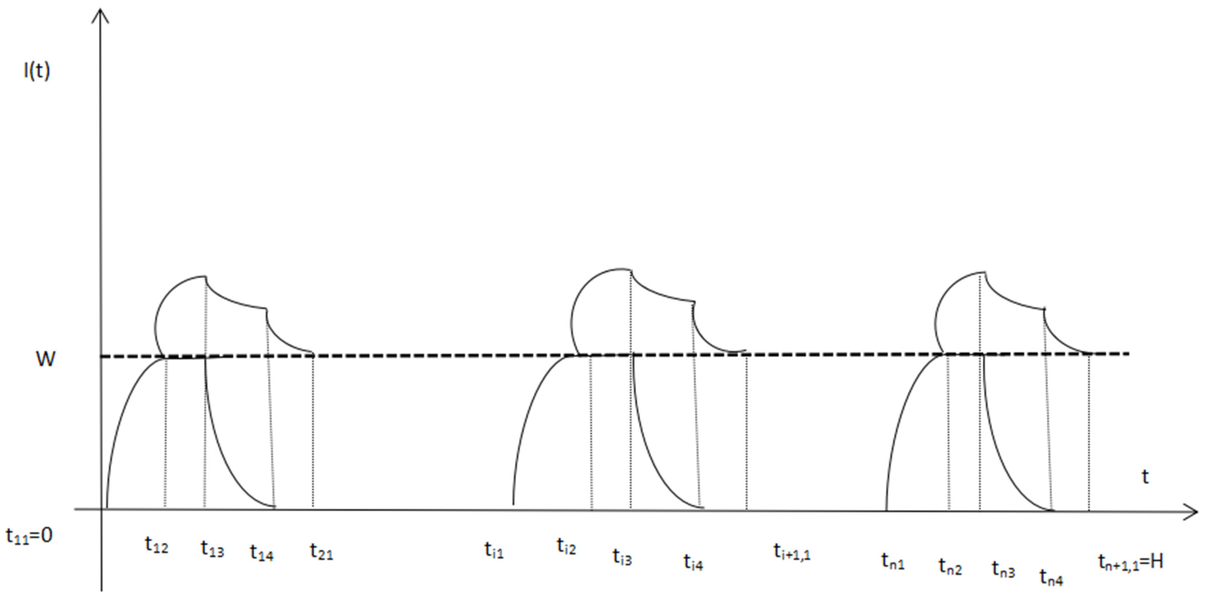
In the present work, a model for deteriorating types of inventories with two-warehousing MFIFO dispatching policy was developed. To design the above-mentioned problem in the form of a mathematical model, regular inspection of items was also considered so as to deduce the deterioration rate. As a result, the deterioration rate depends on the number of inspections. The carbon tax policy for reducing emissions was also considered. The motto of mathematical design is to find the values of n, N and (i = 1, 2, …, N; j = 1, 2, 3, 4) so as to better satisfaction of customer’s demand with the minimum total cost. It is assumed that the ith inventory level initializes at time with null stock level and finishes at time . Initially at time , manufacturing, demand, and deterioration occur simultaneously. The manufacturer using RW for keeping up extra inventories. Figure 1 (Xu et al. 2017) [12] is representing inventory levels in OW and RW in different cycles. Firstly during , manufactured inventories send to the OW where inventory level increases from 0 to W. If there is any extra manufactured inventory more than W after then it must be sent to the RW. If there is any deteriorated inventory in OW during , it arranges or fulfilled from RW. The Manufacturing work stops at , and thereafter, at the inventory level in the OW continuously decreases and reach to 0, because of decay process and demand. Similarly, in the RW, during the inventory level goes down because of decaying process only. After that during , in the RW, the inventory level again goes down due to both decay process and demand. The pattern of changes in the inventory level during supply chain is portrayed in Figure 1. Below established differential equations depict the inventory levels at time t while the ith manufacturing cycle. This work is mainly focused on the deteriorating inventories that need continuous inspection. It is considered that if the deteriorating inventory is removed from the storage, it will not lead to deterioration by contact and the rate of the deterioration slows down. Therefore, the supplier must inspect deteriorating inventory at regular time intervals for removing deteriorating inventory so that it cannot spoil other inventory, and thus removed inventory can be utilized at the initial level.
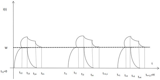
Figure 1.
Representation of inventory level during supply chain.
In this section, basic mathematical equations of inventory level and deteriorated inventories in both OW and RW in different sub-cycles will be calculated. These inventory levels are further used for calculating different costs constructing the final cost model.
With the help of boundary conditions and , the above equation can be solved and model formulation work takes place. The following steps followed:
Here .
Now calculating total inventory level in own warehouse in ith cycle is as follows:
Now calculating total inventory level in rented warehouse in ith cycle is as follows:
3.1. Fixed Manufacturing Cost
This is the fixed manufacturing cost that occurs in the supply chain as a result of the production process and includes activities such as raw materials cost, manufacturing charges, packing, and so on that serve to prepare a product for consumer usage. This is often referred to as the manufacturing cost. It is determined as follows in ith cycle.
3.2. Holding Cost of Desirable Items in OW and RW in ith Cycle
This is the expense incurred in the supply chain as a result of storing prepared stocks in a warehouse. Rent, power bills, maintenance fees, and other expenditures are incurred at a warehouse. For one cycle, the holding cost is determined as follows.
3.3. Deterioration Cost in OW and RW in ith Cycle
Deterioration costs occur as a result of inventory degradation. Inventory deterioration is regarded as a loss for the supply chain. As a result, it is assessed as a degradation cost. The cost of degradation for one cycle is determined as follows:
3.4. Cost of Inspection
The cost of inspection is linearly dependent on the number of inspections per cycle and cost of hiring the number of inspectors, which can be given by:
3.5. Emission Cost
If the inventories’ nature is a deteriorating type, then it will definitely lead to carbon emission. The disposal of deteriorating inventory causes emissions and according to Government policy any business organization that is responsible for carbon emission has to pay the government as a penalty following any one policy established by the Government. In our work we have considered the carbon tax policy. For this let us assume that emissions due to the per unit of disposal of deteriorating inventory be . Emission cost also creates pressure on the supply chain for reducing emission generation.
Therefore, total emission due to deteriorating inventories is:
3.6. Total Cost
Now, the mathematical design for the total cost model under the MFIFO policy is as follows:
In addition, the following relations exist:
We use the Lagrangian method to find the optimal values of:
where are the lagrangian multipliers.
Lemma 1.
For a given cycle number, we prove the uniqueness of the optimal values of tij (i = 1, 2, …, N, j = 1, 2, 3, 4) that satisfy.
Proof.
Refer to Appendix A. □
Now by using Lemma 1 we can write and . With the help of Lemma 1 we can say that is uniquely determined.
Now we can solve the cost optimization problem for the MFIFO dispatching policy with the above-specified constraint.
S.T
Theorem 1.
The cost function is convex with the number of cycle N.
Proof.
To prove the theorem we use the result in our model for cost function and then find . By using a numerical example, it is observed that proves the convexity of total cost with cycle number N. □
4. Numerical Illustration
Here we considered a numerical example to illustrate the established model for a manufacturing supply chain that considered a MFIFO dispatching policy with inspection to remove the deteriorating inventories during cycle as discussed above. Numerical example is:
Here with the use of above numerical values the optimum values of decision variables are:
Now to study the behaviour of the established cost model with decision variables and different parameters and making a conclusive report, we constructed the following Table 1, Table 2 and Table 3. These tables were constructed with slight changes in numerical 1 and optimum values of decision variables. A graphical representation is also given to illustrate the results. An analysis of Table 1, Table 2 and Table 3 and the graphical representation explain the sensitivity analysis and observation section.

Table 1.
Behaviour of total cost with the changes in decision variables.

Table 2.
Behaviour of total cost with the changes in parameters such as , , , , , , .

Table 3.
Changes in with the changes in , , , .
5. Sensitivity Analysis and Observations
- By the mathematical calculation in Table 1 it is observed that as the values of increase, the total cost also increases. This implies that for minimizing the total cost, cycle length and sub cycles should be smaller. If the cycle is smaller then inventories need to be utilized in a limited time to minimize deterioration. Therefore, smaller cycles and sub cycles minimize the total cost and management becomes easy.
- As the value of increases, total cost decreases. This shows that inspection during supply chain for deteriorating inventories is a profitable step. Inspection during supply chain reduces the deterioration rate and reduces deterioration cost. In the same way, this policy reduces carbon emission that also reduces carbon tax; therefore this policy helps to minimize the cost. Along with this, it helps to make a supply chain a green supply chain. It is observed in Table 1 that if we increase , we can minimize the total cost. But it is also observed that when we put total cost decreases, but as we put n = 6 or more the total cost becomes negative; therefore, it is observed that n should be between 3 and 5 for minimum cost.
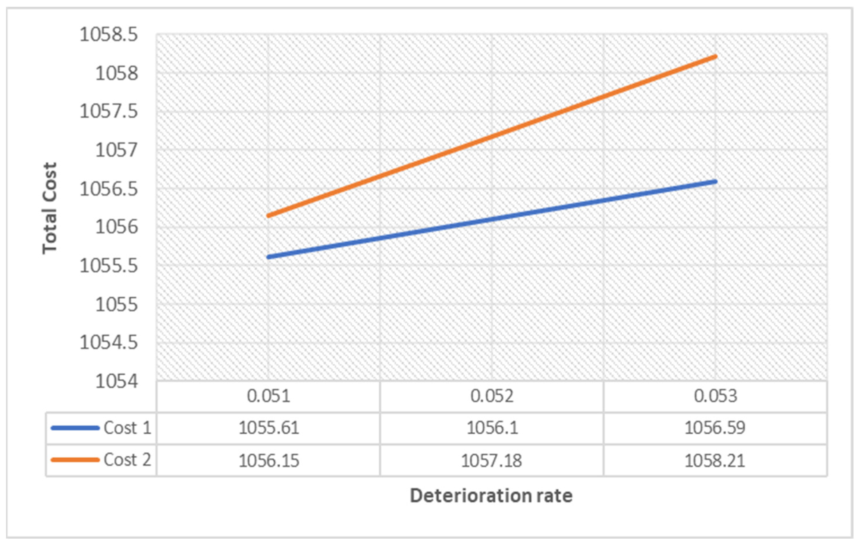
- In Table 2, we studied the behaviour of cost model with respect to the deterioration rate. It is observed that as increases, total cost also increases but when total cost is lower compared to when . Therefore, it is concluded that the deterioration rate should be lower to minimize cost. The same way as we studied the behaviour of total cost with and , it is observed that as increases total cost increases, but when increases total cost decreases.
- Table 3 is constructed by using the result of Lemma 1 which is ; this result gives the value of length of fourth sub cycle.
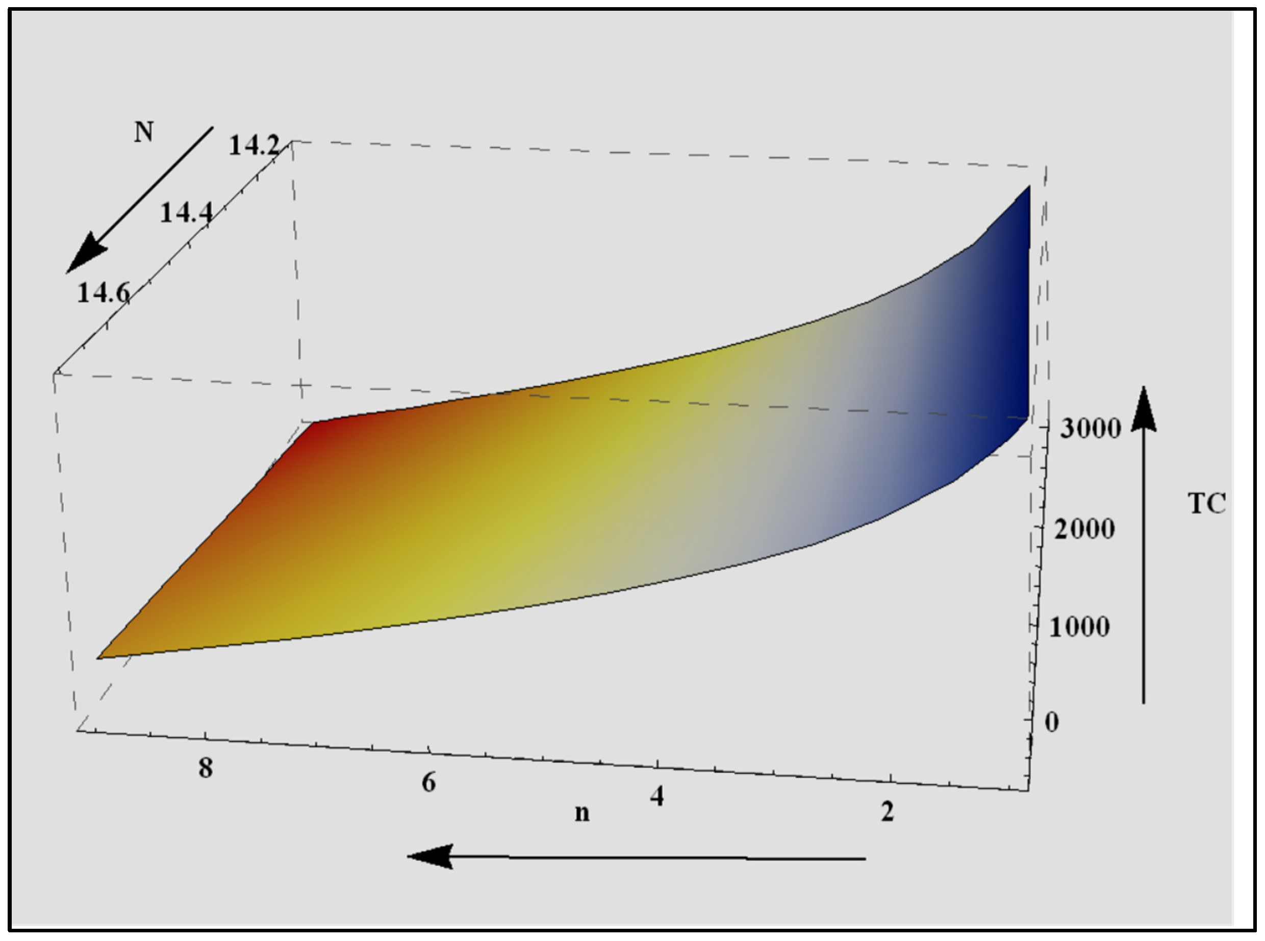
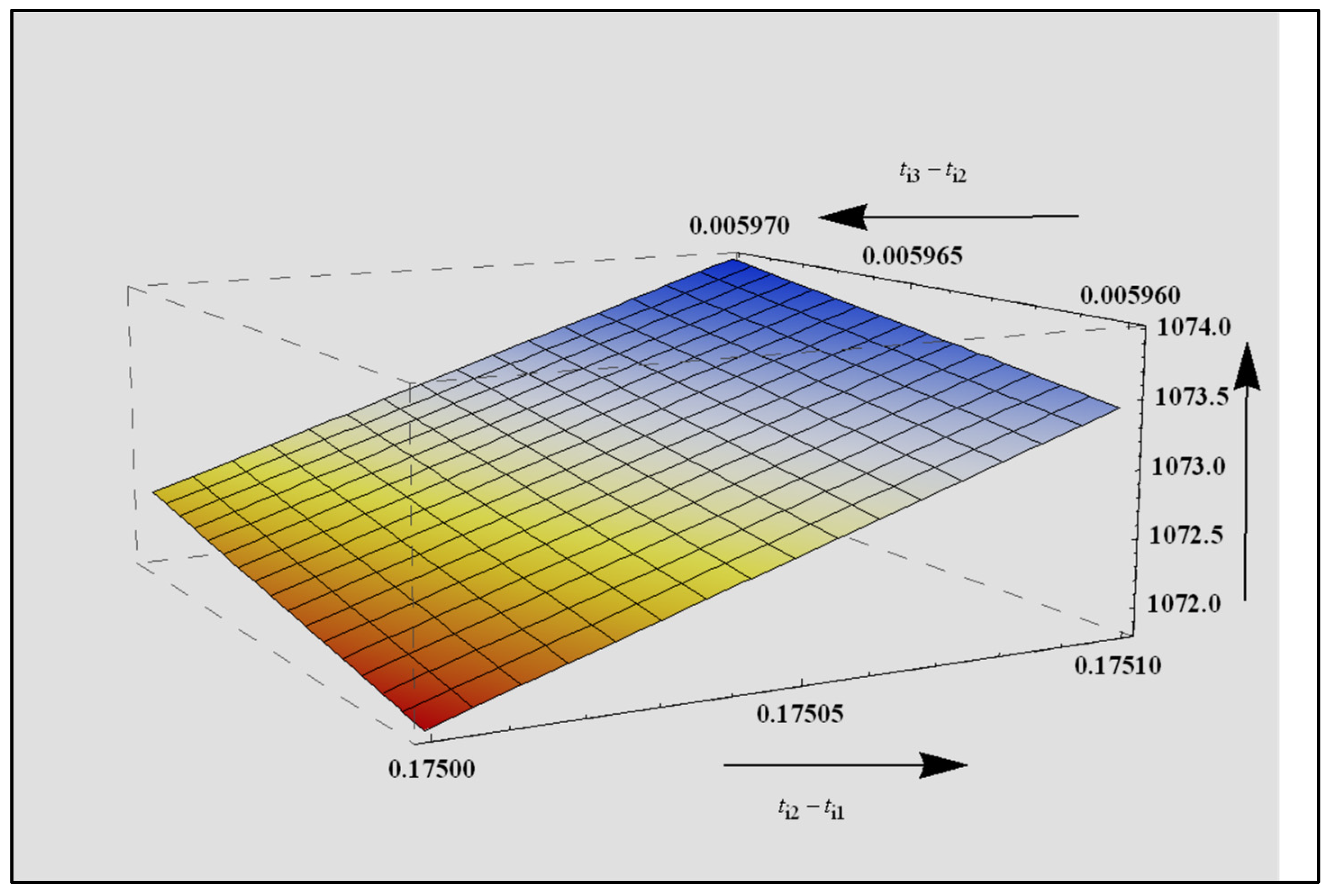
- Figure 2, Figure 3, Figure 4 and Figure 5 shows the behaviour of total cost with respect to different decision variables. Figure 2 represents the behaviour of total cost with respect to . It is observed that the graphical representation also justified our results of Table 1 that the total cost is increasing with increase in (same way with each sub cycle) and decreasing with increases in . Similarly Figure 3 represents the behaviour of total cost with respect to and it is observed that as increases total cost decreases, and as increases the total cost also increases. This supports our results in Table 1. Figure 4 is a graphical representation of total cost with respect to and and it is concluded that with the increase in sub cycle length, total cost increases. Hence, by all the graphical representations and numerical calculations in Table 1 and Table 2, it is observed that total cost increases as increases; therefore to minimize the cost, should be minimized and the number of inspection should be maximized.
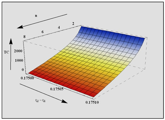 Figure 2. Behaviour of total cost with .
 Figure 3. Behaviour of total cost with .
 Figure 4. Behaviour of total cost with .
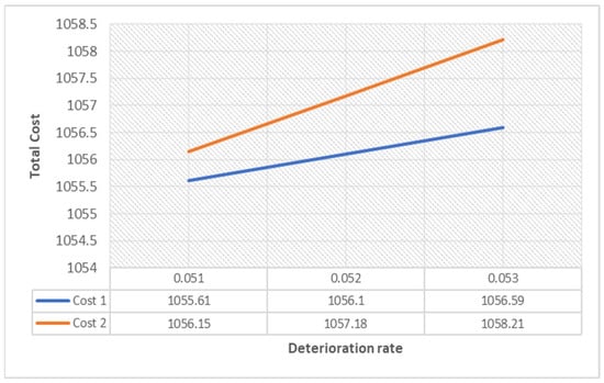 Figure 5. Behaviour of total cost with .
 - Figure 5 represents the behavior of the total cost with respect to the deterioration rate. The graph with blue colour represents the cost when meaning is constant and is increasing whereas the graph with red colour represents the total cost when meaning is constant and is increasing. This graph also concludes that when , TC is lower compared to when .
6. Conclusions
In the present competitive business world organizations need to manage inventories with efficient policies, especially when the supply chain deals with deteriorating inventories. Sometimes due to high demand or season, or any other reasons, the manufacturer increases their production; therefore, in that case they need to manage a large number of inventories with the help of RW. Once the organization rents an extra facility to keep an extra number of inventories, the problem arises regarding which dispatching policy could be best for their supply chain. Along with this the organizations that are dealing with the deteriorating type of inventories need to remove deteriorating inventories at an initial level so as to stop or minimize the deterioration. In this paper, we considered the MFIFO dispatching policy along with inspections. Inspection during supply chain is a perfect tool to convert a supply chain into a green supply chain because it helps to remove deteriorated inventories at the initial level, which helps to stop further decay process by contact. As well, it reduces the problem of disposal of deteriorating inventories because the inventories that are removed can be utilized for any purpose depending on the type of inventories. In our work, we considered inspection policy, constant demand, and deterioration as the function of the number of inspections. By using mathematical modeling it is seen that inspection during supply chain reduces cost. For a given cycle number N, we obtain the uniqueness of the optimal values of . This paper describes an MFIFO policy with inspection and carbon tax policy with the objective of minimizing cost.
Application, Limitations and Further Work
The established mathematical modeling is applicable only on deteriorating types of inventories. It is applicable only if the manufacturer considers only constant demand and making extra inventories due to deteriorating nature inventories. It is not useful if the manufacturer is producing extra inventories due to high demand, due to peak season, because in that case demand will be stochastic, but this model considers only constant demand. Also, it is applicable only for the MFIFO dispatching policy but not applicable if the supply chain follows any other policies. This work can be extended with non-constant demand. In the present paper, we did not discuss the revenue from separated deteriorating inventories as we established a mathematical model to find the total cost; thus, we did not focus on revenues. This work can be extended with a profit model as well.
Author Contributions
Conceptualization, S.S. and H.R.; methodology, S.S. and H.R.; software, H.R. and K.S.; validation, S.S.; formal analysis, S.S.; investigation, K.S.; resources, N.A.; data curation, N.A.; writing—original draft preparation, S.S.; writing—review and editing, N.A. and H.R.; visualization, K.S.; supervision, K.S.; project administration, N.A.; funding acquisition, N.A. All authors have read and agreed to the published version of the manuscript.
Funding
Princess Nourah Bint Abdulrahman University Researchers Supporting Project number (PNURSP2022R59), Princess Nourah Bint Abdulrahman University, Riyadh, Saudi Arabia.
Institutional Review Board Statement
Not applicable.
Informed Consent Statement
Not applicable.
Data Availability Statement
Not applicable.
Acknowledgments
Princess Nourah Bint Abdulrahman University Researchers Supporting Project number (PNURSP2022R59), Princess Nourah Bint Abdulrahman University, Riyadh, Saudi Arabia.
Conflicts of Interest
The authors declare no conflict of interest.
Notation
| Symbol | Description |
| D | Constant demand |
| P | Number of manufactured items |
| The fix rate of deterioration in OW | |
| The effective rate of deterioration in OW | |
| The fix rate of deterioration in RW | |
| The effective rate of deterioration in RW | |
| Stocking charges of inventory in OW | |
| Stocking charges of inventory in RW | |
| Total Stocking charges of inventory in OW | |
| Total Stocking charges of inventory in RW | |
| Maximum limit of OW | |
| Fixed manufacturing cost | |
| Deterioration cost/unit deteriorating inventory | |
| Inventories at time on OW | |
| Inventories at time on OR | |
| Total inventory level in OW in ith manufacturing cycle | |
| Total inventory level in RW in ith manufacturing cycle | |
| Total deteriorating inventory level in OW in ith manufacturing cycle | |
| Total deteriorating inventory level in RW in ith manufacturing cycle | |
| Emission cost | |
| Cost of inspection per cycle | |
| TC | Total cost for one cycle |
| Hiring cost of inspector | |
| Coefficient representing the effect of deteriorated product on desirable product | |
| Tax/unit emission production | |
| Emission/unit due to disposal of a deteriorating product | |
| Decision variables | |
| Initial period of the ith manufacturing cycle along with = 0 and | |
| At this time OW inventory level reaches to its maximum limit W in ith manufacturing cycle where | |
| At this time OR inventory level reaches to its maximum inventory limit and manufacturing work stops in ith manufacturing cycle where | |
| At this time RW inventory level reaches to zero in ith manufacturing cycle where | |
| N | Number of cycles |
| Number of inspections during cycle | |
Appendix A
Here we prove the uniqueness of optimal values of . By using Equation (23).
By using Equations (A1)–(A6), we get the following results.
Substituting Equations (A2), (A3) and (A6) into (A7) we get
By using Equations (A2) and (A9) we get Here we have assume that
By substituting (A10) in (A8)
From Equation (A11), it is concluded that
It is assumed that our model satisfy this condition and we get optimum unique time length in each cycle. On the bases of above proof we can say that each time period is equal to same time point of next cycle. By using (A2) and (A3), we can get and . By using and . It is observed that and . This proof the Lemma 1.
References
- Pal, S.; Mahapatra, G.; Samanta, G. A production inventory model for deteriorating item with ramp type demand allowing inflation and shortages under fuzziness. Econ. Model. 2015, 46, 334–345. [Google Scholar] [CrossRef]
- Bai, Q.; Xu, X.; Xu, J.; Wang, D. Coordinating a supply chain for deteriorating items with multi-factor-dependent demand over a finite planning horizon. Appl. Math. Model. 2016, 40, 9342–9361. [Google Scholar] [CrossRef]
- Muriana, C. An EOQ model for perishable products with fixed shelf life under stochastic demand conditions. Eur. J. Oper. Res. 2016, 255, 388–396. [Google Scholar] [CrossRef]
- Önal, M. The two-level economic lot sizing problem with perishable items. Oper. Res. Lett. 2016, 44, 403–408. [Google Scholar] [CrossRef]
- Wu, J.; Al-Khateeb, F.B.; Teng, J.-T.; Cárdenas-Barrón, L.E. Inventory models for deteriorating items with maximum lifetime under downstream partial trade credits to credit-risk customers by discounted cash-flow analysis. Int. J. Prod. Econ. 2016, 171, 105–115. [Google Scholar] [CrossRef]
- Banerjee, S.; Agrawal, S. Inventory model for deteriorating items with freshness and price dependent demand: Optimal discounting and ordering policies. Appl. Math. Model. 2017, 52, 53–64. [Google Scholar] [CrossRef]
- Feng, L.; Chan, Y.-L.; Cárdenas-Barrón, L.E. Pricing and lot-sizing polices for perishable goods when the demand depends on selling price, displayed stocks, and expiration date. Int. J. Prod. Econ. 2017, 185, 11–20. [Google Scholar] [CrossRef]
- Herbon, A. International Journal of Production Economics Should retailers hold a perishable product having different ages? The case of a homogeneous market and multiplicative demand model. Int. J. Prod. Econ. 2017, 193, 479–490. [Google Scholar] [CrossRef]
- Huber, J.; Gossmann, A.; Stuckenschmidt, H. Cluster-based hierarchical demand forecasting for perishable goods. Expert Syst. Appl. 2017, 76, 140–151. [Google Scholar] [CrossRef]
- Panda, S.; Modak, N.; Cárdenas-Barrón, L.E. Coordination and benefit sharing in a three-echelon distribution channel with deteriorating product. Comput. Ind. Eng. 2017, 113, 630–645. [Google Scholar] [CrossRef]
- Panda, S.; Saha, S.; Modak, N.; Sana, S. A volume flexible deteriorating inventory model with price sensitive demand. Tékhne 2017, 15, 117–123. [Google Scholar] [CrossRef]
- Xu, X.; Bai, Q.; Chen, M. A comparison of different dispatching policies in two-warehouse inventory systems for deteriorating items over a finite time horizon. Appl. Math. Model. 2017, 41, 359–374. [Google Scholar] [CrossRef]
- Aliyu, I.; Sani, B. An Inventory Model for Deteriorating Items with Generalised Exponential Decreasing Demand, Constant Holding Cost and Time-Varying Deterioration Rate. Am. J. Oper. Res. 2018, 8, 1–16. [Google Scholar] [CrossRef][Green Version]
- Ferreira, G.O.; Arruda, E.; Marujo, L.G. Inventory management of perishable items in long-term humanitarian operations using Markov Decision Processes. Int. J. Disaster Risk Reduct. 2018, 31, 460–469. [Google Scholar] [CrossRef]
- Pando, V.; San-José, L.A.; García-Laguna, J.; Sicilia, J. Optimal lot-size policy for deteriorating items with stock-dependent demand considering profit maximization. Comput. Ind. Eng. 2018, 117, 81–93. [Google Scholar] [CrossRef]
- Rozhkov, M.; Ivanov, D. Contingency Production-Inventory Control Policy for Capacity Disruptions in the Retail Supply Chain with Perishable Products. IFAC-PapersOnLine 2018, 51, 1448–1452. [Google Scholar] [CrossRef]
- Tiwari, S.; Jaggi, C.K.; Gupta, M.; Cárdenas-Barrón, L.E. Optimal pricing and lot-sizing policy for supply chain system with deteriorating items under limited storage capacity. Int. J. Prod. Econ. 2018, 200, 278–290. [Google Scholar] [CrossRef]
- Tiwari, S.; Cárdenas-Barrón, L.E.; Shaikh, A.A.; Goh, M. Retailer’s optimal ordering policy for deteriorating items under order-size dependent trade credit and complete backlogging. Comput. Ind. Eng. 2020, 139, 105559. [Google Scholar] [CrossRef]
- Bai, Q.; Gong, Y.; Jin, M.; Xu, X. Effects of carbon emission reduction on supply chain coordination with vendor-managed deteriorating product inventory. Int. J. Prod. Econ. 2018, 208, 83–99. [Google Scholar] [CrossRef]
- Jing, F.; Mu, Y. Forecast horizon for dynamic lot sizing model under product substitution and perishable inventories. Comput. Oper. Res. 2019, 110, 77–87. [Google Scholar] [CrossRef]
- Maihami, R.; Govindan, K.; Fattahi, M. The inventory and pricing decisions in a three-echelon supply chain of deteriorating items under probabilistic environment. Transp. Res. Part E Logist. Transp. Rev. 2019, 131, 118–138. [Google Scholar] [CrossRef]
- Yang, Y.; Chi, H.; Tang, O.; Zhou, W.; Fan, T. Cross perishable effect on optimal inventory preservation control. Eur. J. Oper. Res. 2019, 276, 998–1012. [Google Scholar] [CrossRef]
- Khakzad, A.; Gholamian, M.R. The effect of inspection on deterioration rate: An inventory model for deteriorating items with advanced payment. J. Clean. Prod. 2020, 254, 120117. [Google Scholar] [CrossRef]
- Halim, M.A.; Paul, A.; Mahmoud, M.; Alshahrani, B.; Alazzawi, A.Y.; Ismail, G.M. An overtime production inventory model for deteriorating items with nonlinear price and stock dependent demand. Alex. Eng. J. 2021, 60, 2779–2786. [Google Scholar] [CrossRef]
- Chakraborty, D.; Jana, D.K.; Roy, T.K. Two-warehouse partial backlogging inventory model with ramp type demand rate, three-parameter Weibull distribution deterioration under inflation and permissible delay in payments. Comput. Ind. Eng. 2018, 123, 157–179. [Google Scholar] [CrossRef]
- Niu, B.; Xie, J. A note on “Two-warehouse inventory model with deterioration under FIFO dispatch policy”. Eur. J. Oper. Res. 2008, 190, 571–577. [Google Scholar] [CrossRef]
- Yu, J.C. Optimizing a two-warehouse system under shortage backordering, trade credit, and decreasing rental conditions. Int. J. Prod. Econ. 2019, 209, 147–155. [Google Scholar] [CrossRef]
- Ghiami, Y.; Beullens, P. The continuous resupply policy for deteriorating items with stock-dependent observable demand in a two-warehouse and two-echelon supply chain. Appl. Math. Model. 2020, 82, 271–292. [Google Scholar] [CrossRef]
- Minner, S.; Transchel, S. Order variability in perishable product supply chains. Eur. J. Oper. Res. 2017, 260, 93–107. [Google Scholar] [CrossRef]
- Janssen, L.; Diabat, A.; Sauer, J.; Herrmann, F. A stochastic micro-periodic age-based inventory replenishment policy for perishable goods. Transp. Res. Part E Logist. Transp. Rev. 2018, 118, 445–465. [Google Scholar] [CrossRef]
- Alamri, A.A.; Syntetos, A.A. Beyond LIFO and FIFO: Exploring an Allocation-In-Fraction-Out (AIFO) policy in a two-warehouse inventory model. Int. J. Prod. Econ. 2018, 206, 33–45. [Google Scholar] [CrossRef]
- Jaber, M.Y.; Goyal, S. A basic model for coordinating a four-level supply chain of a product with a vendor, multiple buyers and tier-1 and tier-2 suppliers. Int. J. Prod. Res. 2009, 47, 3691–3704. [Google Scholar] [CrossRef]
- Mishra, U.; Wu, J.-Z.; Tsao, Y.-C.; Tseng, M.-L. Sustainable inventory system with controllable non-instantaneous deterioration and environmental emission rates. J. Clean. Prod. 2019, 244, 118807. [Google Scholar] [CrossRef]
- Wang, M.; Zhao, L.; Herty, M. Joint replenishment and carbon trading in fresh food supply chains. Eur. J. Oper. Res. 2019, 277, 561–573. [Google Scholar] [CrossRef]
- Wu, T.; Kung, C.-C. Carbon emissions, technology upgradation and financing risk of the green supply chain competition. Technol. Forecast. Soc. Chang. 2019, 152, 119884. [Google Scholar] [CrossRef]
- Bhatia, M.S.; Jakhar, S.K.; Mangla, S.K.; Gangwani, K.K. Critical factors to environment management in a closed loop supply chain. J. Clean. Prod. 2020, 255, 120239. [Google Scholar] [CrossRef]
- Huang, Y.-S.; Fang, C.-C.; Lin, Y.-A. Computers & Industrial Engineering Inventory management in supply chains with consideration of Logistics, green investment and different carbon emissions policies. Comput. Ind. Eng. 2019, 139, 106207. [Google Scholar] [CrossRef]
- Yu, C.; Qu, Z.; Archibald, T.W.; Luan, Z. An inventory model of a deteriorating product considering carbon emissions. Comput. Ind. Eng. 2020, 148, 106694. [Google Scholar] [CrossRef]
- Mishra, U.; Wu, J.-Z.; Sarkar, B. Optimum sustainable inventory management with backorder and deterioration under controllable carbon emissions. J. Clean. Prod. 2020, 279, 123699. [Google Scholar] [CrossRef]
- Sepehri, A.; Gholamian, M.R. Joint pricing and lot-sizing for a production model under controllable deterioration and carbon emissions. Int. J. Syst. Sci. Oper. Logist. 2021, 9, 324–338. [Google Scholar] [CrossRef]
- Mohammadi, B.; Taleizadeh, A.A.; Noorossana, R.; Samimi, H. Optimizing integrated manufacturing and products inspection policy for deteriorating manufacturing system with imperfect inspection. J. Manuf. Syst. 2015, 37, 299–315. [Google Scholar] [CrossRef]
- Tai, A.H.; Xie, Y.; Ching, W.-K. Inspection policy for inventory system with deteriorating products. Int. J. Prod. Econ. 2016, 173, 22–29. [Google Scholar] [CrossRef]
- Bouslah, B.; Gharbi, A.; Pellerin, R. Joint economic design of production, continuous sampling inspection and preventive maintenance of a deteriorating production system. Int. J. Prod. Econ. 2016, 173, 184–198. [Google Scholar] [CrossRef]
- Tai, A.H.; Xie, Y.; He, W.; Ching, W.-K. Joint inspection and inventory control for deteriorating items with random maximum lifetime. Int. J. Prod. Econ. 2019, 207, 144–162. [Google Scholar] [CrossRef]
Publisher’s Note: MDPI stays neutral with regard to jurisdictional claims in published maps and institutional affiliations. |
© 2022 by the authors. Licensee MDPI, Basel, Switzerland. This article is an open access article distributed under the terms and conditions of the Creative Commons Attribution (CC BY) license (https://creativecommons.org/licenses/by/4.0/).

