Application of Extended Set Pair Analysis on Wear Risk Evaluation of Backfill Pipeline

Abstract

Filling slurry can inevitably cause irreversible wear to the pipeline, which represents great costs to mines. This study aims to propose an extended set pair analysis (SPA) for the wear risk evaluation of backfill pipeline. First, to fully describe the wear risk of backfill pipeline, an evaluation index system was established from the aspects of slurry characteristics, pipeline properties, and slurry flow state. Then, the experts grading method was modified with probabilistic linguistic term sets (PLTSs) to obtain subjective weights. Meanwhile, the criteria importance through intercriteria correlation (CRITIC) approach was used to calculate objective weights. By introducing a preference coefficient, they were integrated to determine the comprehensive weights. After that, the classical SPA was extended with membership functions and fuzzy entropy theory, so that the wear risk of backfill pipeline can be evaluated from the perspectives of both the risk level and complexity. Finally, the proposed methodology was applied to assess the wear risk in the Jinchuan nickel mine, Dahongshan copper mine, Hedong gold mine, and Xincheng gold mine. The reliability of evaluation results was further verified through sensitivity and comparative analyses. Results indicate that the proposed methodology is feasible for the wear risk evaluation of backfill pipeline, and can provide guidance on the wear risk management.

1. Introduction

Due to the requirements of safety and environmental protection, the backfill mining method has been widely used in underground mines [1,2,3]. With the increase in mining depth, the safety, stability and reliability of filling systems have become more and more important. The backfill pipeline, which plays the role of transporting filling slurry from surface filling stations to underground stopes, is a key part [4]. However, the filling slurry can wear and even break the pipeline during long-distance transportations [5,6]. It not only affects the normal production and economic benefits of mines, but also may lead to major safety accidents. Then, the sustainability of mines can be greatly affected. Therefore, assessing the wear risk of backfill pipeline is crucial and meaningful for risk management.

Plenty of research has been conducted on the wear characteristics of backfill pipeline. Steward and Spearing [7] summarized the factors that affected the wear of pipeline. Cooke [8] deemed that the movement of particles on the pipeline wall included abrasion and erosion, and then classified the wear modes into deformation and cutting wear. McGuinness and Cooke [9] identified the issues related to the thinning of pipeline walls, which can cause undesirable safety concerns and severe localized wear. Hewitt et al. [10] determined the relationship between pipe material and wear rate based on the pipe lining abrasion testing, and found that the pipe material was significantly important for the availability of the backfill system. Zhang et al. [11] analyzed the wear mechanism of vertical backfill pipeline from the perspective of momentum and energy, and deemed that the wear position was in the interface between air and solid-liquid mixture. Gharib et al. [12] evaluated the flow and wear characteristics in pipe elbows by combining analytical solutions, experimental and numerical simulation methods, and discovered elbow design and slurry property had large influences on pipe wear rate. Wang et al. [13] invested the wear of backfill pipelines in Jinchuan nickel mine, and summarized the main influencing factors of pipeline wear. Creber et al. [14] measured the wear rate of backfill pipeline in four Canadian mines, and found the selection of backfill materials can significantly influence wear rate. This research provide foundations for the determination of wear risk evaluation indexes.

Recently, numerous mathematical models have been developed to assess the wear risk of backfill pipeline, which can be summarized into two types. The first one is the machine learning algorithm. Li and Nie [15] integrated the kernel principal component analysis, particle swarm optimization and generalized regression neural network to tackle wear risk issues of backfill pipeline. Guo and Zhang [16] adopted the principal component analysis and back propagation neural network to establish backfill pipeline wear risk evaluation models. Luo et al. [17] introduced an improved particle swarm optimization to optimize the least squares support vector machine for the wear risk prediction of backfill pipeline. These algorithms can well establish the nonlinear relationship between the wear risk level and evaluation indexes, but a large amount of data is required to improve the reliability. The second one is the multi-criteria evaluation approach. Zhang et al. [18] evaluated the reliability of backfill pipeline based on extenics theory. Xue et al. [19] selected twelve evaluation indexes, and proposed an integrated model of combination weights and variable fuzzy sets to evaluate backfill pipeline wear risk. Wang et al. [20] adopted fourteen influencing factors, and used cloud model to predict wear risk of vertical filling pipes. Ding et al. [21] chose twelve indicators, and established the evaluation model of wear risk based on the improved unascertained measurement method. These approaches can simultaneously consider the influence of qualitative and quantitative indexes, and effectively determine the specific risk levels. However, the index weights and the risk rating standards should be determined in advance.

Except for above methods, set pair analysis (SPA) is another effective quantitative assessment method. Due to the simple calculation steps, objective evaluation results and superiority in dealing with both certainty and uncertainty, it has been widely used in a range of fields. For example, Guo et al. [22] integrated an improved SPA and variable fuzzy set to assess the risk of flood disaster. Chong et al. [23] used the analytic hierarchy process, gray model theory, and SPA to deal with occupational hazard problems of coal mining. Roy and Datta [24] adopted the entropy theory and SPA to achieve adaptive management of coastal aquifers. Giao et al. [25] classified the water quality in Vietnamese Mekong delta based on SPA and Vietnamese water quality index. Zhang and Li [26] combined the projection pursuit method and improved SPA to assess the construction risk of deep foundation pit. Zhao et al. [27] combined analytic hierarchy process, entropy weight method and SPA to identify the source of water inrush. Wang et al. [28] used combination weighting method and SPA to establish the risk assessment model of airport bird strikes. Considering the effectiveness of SPA has been proved in various studies, it may be suggested to evaluate the wear risk of backfill pipelines. However, two key issues need to be addressed for the classical SPA. One is the determination of connection degree expression, and another one is the judgment of the difference between samples with the same risk level but with different connection numbers. To address these two issues, the membership function in fuzzy theory can be firstly introduced to determine the connection degree [29]. Thereafter, the fuzzy entropy of connection numbers can be used to reflect the inherent ambiguity of information [30]. In this case, the sample can be evaluated from the perspectives of both the risk level and complexity.

The aim of this study is to propose an extended SPA for the wear risk evaluation of backfill pipeline. First, the wear risk evaluation index system of backfill pipeline is established. Then, the extended experts grading method with probabilistic linguistic term sets (PLTSs), and criteria importance through intercriteria correlation (CRITIC) approach are combined to calculate the index weights. After that, the SPA is extended to evaluate the wear risk from both the risk level and complexity. Finally, the proposed methodology is applied to assess the wear risk in four mines.

2. Evaluation Indexes of Wear Risk

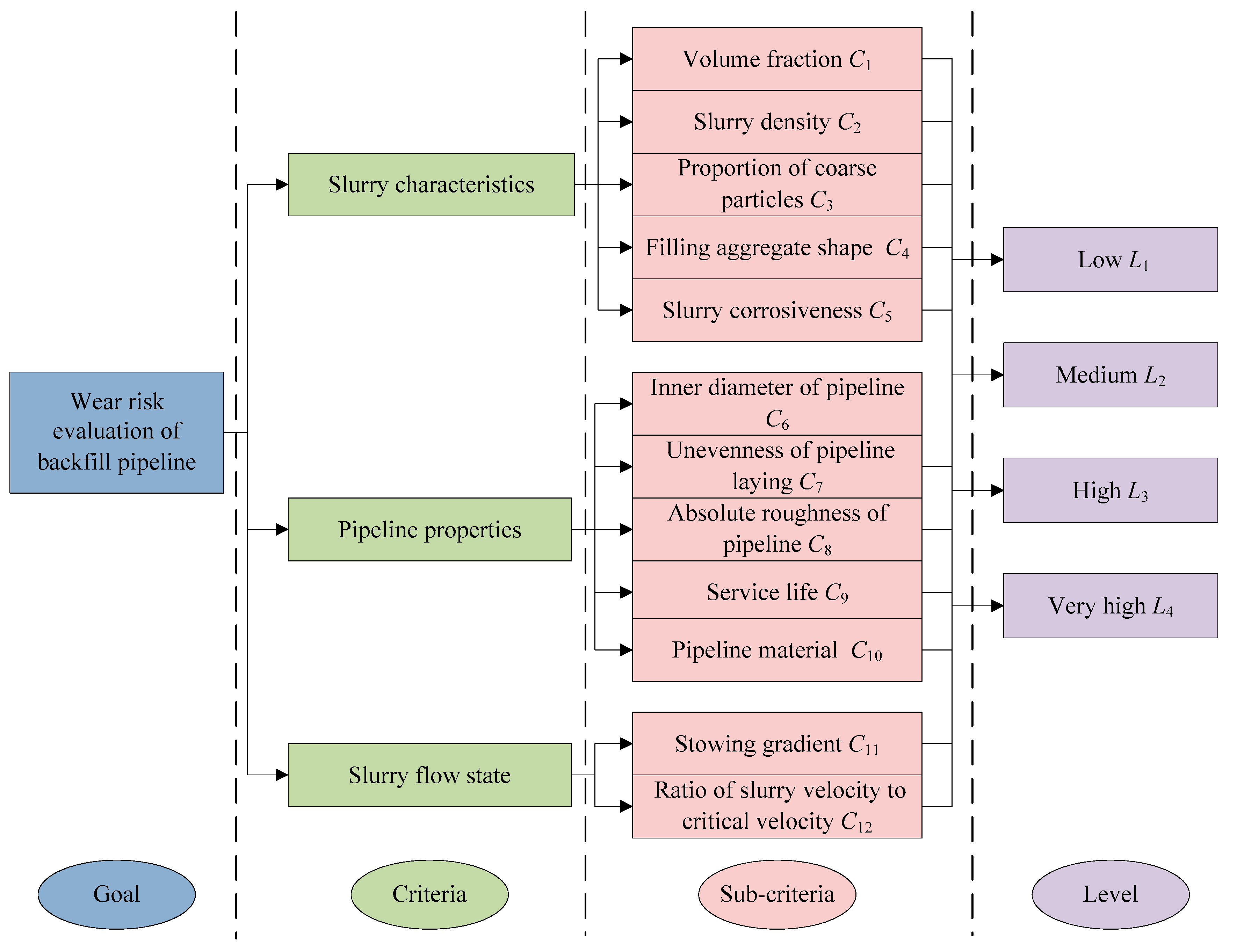
Selecting appropriate indexes is essential for the wear risk evaluation of backfill pipeline. Due to the complexity of influencing factors, a standard evaluation index system has not been formed. Based on the wear mechanism of backfill pipeline, evaluation indexes are selected from three criteria, including slurry characteristics, pipeline properties, and slurry flow state. The index system for the wear risk evaluation of backfill pipeline is shown in Figure 1.

(1)

Slurry characteristics

Since pipeline wear is caused by the friction between the filling slurry and pipeline wall, it is true that the wear risk is related to the slurry characteristics [7,31,32]. In general, the volume fraction, density, proportion of coarse particles, aggregate shape, and corrosiveness of slurry have large influences on pipeline wear. Therefore, the sub-criteria of slurry characteristics include the volume fraction (denoted as $C_1$), slurry density (denoted as $C_2$), proportion of coarse particles (denoted as $C_3$), filling aggregate shape (denoted as $C_4$), and slurry corrosiveness (denoted as $C_5$). The wear rate of pipeline elevates with the increase in $C_1$, $C_2$, and $C_3$. The more irregular the shape of the filling aggregate, the greater the pipeline wear. In addition, the slurry corrosiveness will accelerate the wear of pipeline.

(2)

Pipeline properties

Under the same slurry characteristics, the wear is closely related to the properties of the selected pipeline [7,33,34]. The inner diameter, installation quality, absolute roughness, service life, and material affect the pipeline wear greatly. Therefore, the sub-criteria of pipeline properties include the inner diameter of pipeline (denoted as $C_6$), unevenness of pipeline laying (denoted as $C_7$), absolute roughness of pipeline (denoted as $C_8$), service life (denoted as $C_9$), and pipeline material (denoted as $C_{10}$). The wear rate of pipeline decreases with the increase in $C_6$. The larger the $C_7$, $C_8$, and $C_9$, the lower the pipeline wear. Moreover, the service life of pipeline with wear-resistant lining is several times that of ordinary steel pipeline.

(3)

Slurry flow state

The wear of pipeline is different when the slurry flow state is dissimilar. The slurry flow state is affected by many factors, such as the stowing gradient and the ratio of slurry velocity to critical velocity [16,17,19]. Stowing gradient indicates the ratio of the total length to the height difference between the start and end of the pipeline. If the stowing gradient is too small, the wear will get worse with the increase in slurry impact force on pipeline. In addition, the greater the ratio of slurry velocity to critical velocity, the more severe the wear. Therefore, the sub-criteria of slurry flow state include the stowing gradient (denoted as $C_{11}$) and the ratio of slurry velocity to critical velocity (denoted as $C_{12}$).

According to the severity of pipeline wear, the risk is classified into four levels, including low ($L_1$), medium ($L_2$), high ($L_3$), and very high ($L_4$). To assess pipeline wear risk, the index values corresponding to these four levels are indicated, as shown in

Table 1. Classification standards of each index [35].

Indexes	Levels
	L1	L2	L3	L4
$C_1$/%	<30	30–40	40–50	>50
$C_2$/t/m3	<1.5	1.5–1.7	1.7–1.9	>1.9
$C_3$/%	<20	20–40	40–60	>60
$C_4$	Round or oval	Square	Polygonal	Extremely irregular shape
$C_5$	Neutral and free of ingredients that can react with the pipeline	pH changes under specific conditions, causing reaction with the pipeline	Weak acids, bases and other ingredients that react slightly with the pipeline	Strong acids, bases and other ingredients that readily react with the pipeline
$C_6$/mm	>200	150–200	100–150	<100
$C_7$/%	<1.0	1.0–3.0	3.0–5.0	>5.0
$C_8$/μm	<100	100–300	300–500	>500
$C_9$/a	<2	2–5	5–10	>10
$C_{10}$	Bimetal wear-resistant composite pipeline	Steel-plastic composite pipeline	Ceramic composite pipeline	Single composite material
$C_{11}$	>7.0	5.0–7.0	3.0–5.0	<3.0
$C_{12}$	<1.0	1.0–1.2	1.2–1.5	>1.5

[35]. It can be seen that the index system includes nine quantitative indexes ($C_1$, $C_2$, $C_3$, $C_6$, $C_7$, $C_8$, $C_9$, $C_{11}$ and $C_{12}$) and three qualitative indexes ($C_4$, $C_5$ and $C_{10}$). To facilitate evaluation, the scores of qualitative indexes for level $L_1$, $L_2$, $L_3$ and $L_4$ are selected as 1, 2, 3, and 4, respectively.

3. Methodology

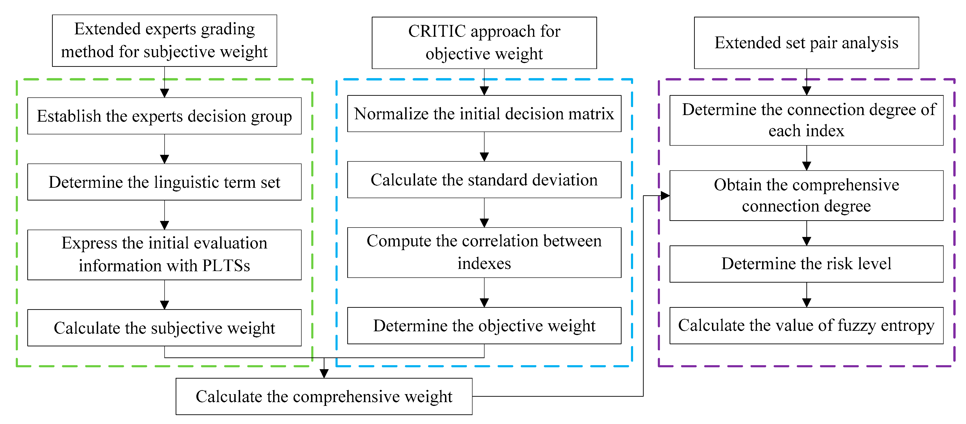
A novel methodology for the wear risk evaluation of backfill pipeline is proposed in this section. It mainly includes two phases, as shown in Figure 2. First, the comprehensive weight is calculated based on an extended experts grading method and CRITIC approach. Then, the wear risk of backfill pipeline is determined by the extended SPA. The details of these two phases are described as follows.

3.1. Comprehensive Weight Method

(1)

Extended experts grading method for subjective weight

The subjective weight is determined based on the extended experts grading method with PLTSs. The specific steps are as follows:

Step 1: Determine the linguistic term set

In reality, experts tend to use linguistic phrases to indicate the importance of indicators [36,37]. In this study, the linguistic term set is selected as: very unimportant, unimportant, slightly unimportant, medium, slightly important, important, and very important. In general, the linguistic term set can be denoted by

$$S=\left\{s_a|a=-p,\dots ,-1,0,1,\dots ,p\right\}$$

(1)

where $s_a$ is a linguistic variable, and the number of linguistic variables is $2p+1$. Particularly, $s_{-p}$ and $s_p$ represent the lower and upper limits of linguistic variables, respectively.

Then, the linguistic term set in this study can be indicated as

$$S=\left\{\begin{array}{l}{s}_{-3}=\mathrm{very} \mathrm{unimportant},s_{-2}=\mathrm{unimportant},s_{-1}=\mathrm{slightly} \mathrm{unimportant},s_0=\mathrm{medium},\\ s_1=\mathrm{slightly} \mathrm{important},s_2=\mathrm{important},s_3=\mathrm{very} \mathrm{important}\end{array}\right\}$$

Step 2: Express the initial evaluation information with PLTSs

Based on the selected linguistic term set, experts can evaluate the importance of each index individually and anonymously. To fully describe the original evaluation information, these linguistic phrases can be expressed by PLTSs [38]. For example, the probabilistic linguistic term set (PLTS) $\left\{s_{-1}(0.1),s_1(0.3),s_2(0.6)\right\}$ indicates 10% experts believe it is slightly unimportant, 30% experts believe it is slightly important, and 60% experts believe it is important.

Step 3: Calculate the subjective weight

Given a linguistic term set $S$, the PLTS can be indicated as [39]

$$T(b)=\left\{T^{(k)}(b^{(k)})|T^{(k)}\in S,b^{(k)}\ge 0,k=1,2,\dots ,K,{\displaystyle {\sum }_{k=1}^K{b}^{(k)}\le 1}\right\}$$

(2)

where $T^{(k)}(b^{(k)})$ is the linguistic variable $T^{(k)}$ related to the probabilistic information $b^{(k)}$, and $K$ is the number of linguistic variables in $T(b)$.

The score function of $T(b)$ can be determined by [39]

$$F(T(b))=\frac{1}{{\displaystyle {\sum }_{k=1}^K{b}^{(k)}}}{\displaystyle {\sum }_{k=1}^K{b}^{(k)}{T}^{(k)}}$$

(3)

Then, the subjective weight can be calculated by

$${\omega }_q^s=\frac{e_q}{{\displaystyle \sum _q^n{e}_q}}$$

(4)

where $e_q$ is the subscript of linguistic term $F{(T(b))}_q$, $q$ is the indicator number, and $q=1,2,\dots ,n$.

(2)

CRITIC approach for objective weight

The CRITIC approach proposed by Diakoulaki et al. [40] is used to calculate the objective weight. The weight is determined based on the intrinsic fluctuation information of data. This method adopted the standard deviation and correlation coefficient to reflect the volatility and correlation, respectively. If the standard deviation is larger, and the correlation coefficient is smaller, the weight will be higher. The specific steps are as follows [41,42]:

Step 1: Normalize the initial decision matrix

Suppose the initial decision matrix is

$$X=\left[\begin{array}{cccc}{x}_{11}& x_{12}& \cdots & x_{1n}\\ x_{21}& x_{22}& \cdots & x_{2n}\\ ⋮& ⋮& \ddots & ⋮\\ x_{m1}& x_{m2}& \cdots & x_{mn}\end{array}\right]$$

(5)

where $x_{pq}$ indicates the value of sample $B_p$ ($p=1,2,\dots ,m$) with respect to index $C_q$ ($q=1,2,\dots ,n$).

To eliminate the influence of dimensions, the initial decision matrix should be normalized by

$$x_{pq}^{\prime }=\left\{\begin{array}{l}\frac{x_{pq}-\underset{q}{\min }(x_{pq})}{\underset{q}{\max }(x_{pq})-\underset{q}{\min }(x_{pq})} \mathrm{for} \mathrm{benefit} \mathrm{indexes}\\ \frac{\underset{q}{\max }(x_{pq})-x_{pq}}{\underset{q}{\max }(x_{pq})-\underset{q}{\min }(x_{pq})} \mathrm{for} \cos \mathrm{t} \mathrm{indexes}\end{array}\right.$$

(6)

Step 2: Calculate the standard deviation

$$S_q=\sqrt{\frac{{\displaystyle \sum _{p=1}^m{(x_{pq}^{\prime }-{\overline{x}}_q)}^2}}{m-1}}$$

(7)

where ${\overline{x}}_q$ is the average value of index $C_q$ for all samples.

Step 3: Compute the correlation between indexes

$$R_q={\displaystyle \sum _{h=1}^n(1-r_{qh})}$$

(8)

where $r_{qh}$ indicates the Pearson correlation coefficient between index $C_q$ and $C_h$.

Step 4: Determine the objective weight

$${\omega }_q^o=\frac{S_q{R}_q}{{\displaystyle \sum _{q=1}^n{S}_q{R}_q}}$$

(9)

(3)

Calculate the comprehensive weight

Based on the subjective and objective weights, the comprehensive weight can be obtained by

$${\omega }_q=\lambda {\omega }_q^s+(1-\lambda ){\omega }_q^o$$

(10)

where $0\le \lambda \le 1$ is a preference coefficient. If the importance of subjective and objective weights is equivalent, then $\lambda =0.5$.

3.2. Extended Set Pair Analysis

SPA is a systematic analysis method for dealing with uncertain problems [43]. The core idea is to regard the certainty and uncertainty of things as a system. In this system, the certainty is divided into identity and contrary, and the uncertainty is called discrepancy. By introducing the concept of connection degree, the uncertainties caused by randomness, ambiguity and incomplete information are indicated uniformly [25,26].

Generally, the connection degree of two sets can be expressed by

$$\mu =\alpha +\beta i+\gamma j$$

(11)

where $\alpha$, $\beta$ and $\gamma$ are the connection numbers, which indicate the degree of identity, discrepancy and contrary, respectively, and $\alpha +\beta +\gamma =1$, $i$ is the uncertainty coefficient, and $j$ is the contradictory coefficient.

In addition, based on the developability principle, the connection degree can be extended to meet the needs of actual application

$$\mu =\alpha +{\beta }_1{i}_1+{\beta }_2{i}_2+\cdots +{\beta }_{Z-2}{i}_{Z-2}+\gamma j$$

(12)

where ${\beta }_k\ge 0$$(k=1,2,\cdots ,Z-2)$ represents the different levels of discrepancy degree, and $\alpha +{\beta }_1+{\beta }_2+\cdots {\beta }_{Z-2}+\gamma =1$.

The specific steps of the extended SPA are as follows:

Step 1: Determine the connection degree of each index

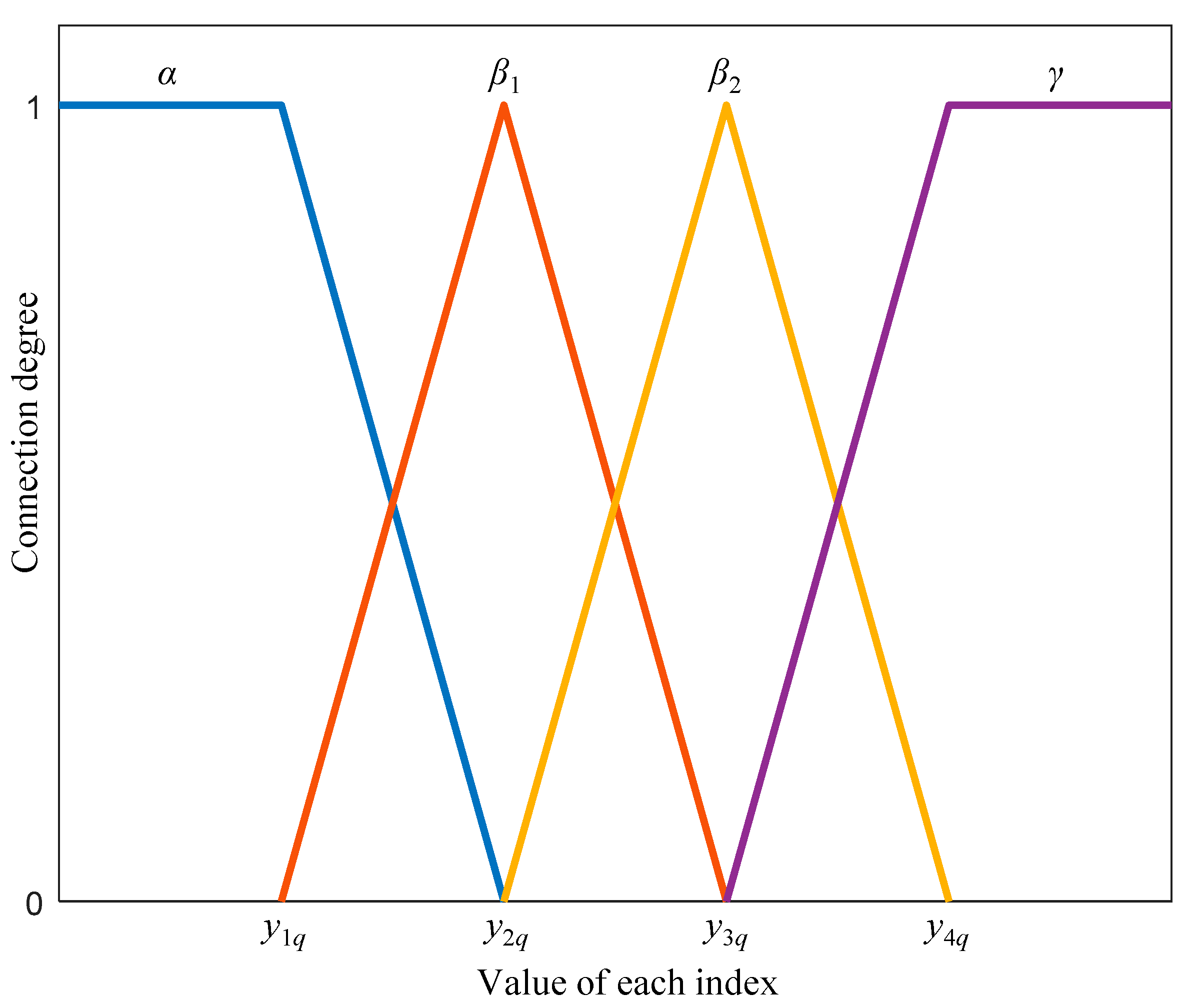
The triangle membership function is used to determine the connection degree. For benefit indexes, the expression is

$${\mu }_q=\left\{\begin{array}{c}1+0i_1+0i_2+\cdots +0i_{Z-2}+0j\left(x_{pq}\ge y_{1q}\right)\hfill \\ \frac{x_{pq}-y_{2q}}{y_{1q}-y_{2q}}+\frac{y_{1q}-x_{pq}}{y_{1q}-y_{2q}}{i}_1+0i_2+\cdots +0i_{Z-2}+0j\left(y_{2q}\le x_{pq}<y_{1q}\right)\hfill \\ 0+\frac{x_{pq}-y_{3q}}{y_{2q}-y_{3q}}{i}_1+\frac{y_{2q}-x_{pq}}{y_{2q}-y_{3q}}{i}_2+\cdots +0i_{Z-2}+0j\left(y_{3q}\le x_{pq}<y_{2q}\right)\hfill \\ ⋮\hfill \\ 0+0i_1+0i_2+\cdots +\frac{x_{pq}-y_{Zq}}{y_{(Z-1)q}-y_{Zq}}{i}_{Z-2}+\frac{y_{(Z-1)q}-x_{pq}}{y_{(Z-1)q}-y_{Zq}}j\left(y_{Zq}\le x_{pq}<y_{(Z-1)q}\right)\hfill \\ 0+0i_1+0i_2+\cdots +0i_{Z-2}+1j\left(x_{pq}<y_{Zq}\right)\hfill \end{array}\right.$$

(13)

where $y_{1q}$, $y_{2q}$, $y_{3q}$, $y_{(Z-1)q}$, and $y_{Zq}$ indicate the limit values of index $C_q$ for risk level $L_1$, $L_2$, $L_3$, $L_{Z-1}$, and $L_Z$, respectively.

For cost indexes, the expression is

$${\mu }_q=\left\{\begin{array}{c}1+0i_1+0i_2+\cdots +0i_{Z-2}+0j\left(x_{pq}\le y_{1q}\right)\hfill \\ \frac{y_{2q}-x_{pq}}{y_{2q}-y_{1q}}+\frac{x_{pq}-y_{1q}}{y_{2q}-y_{1q}}{i}_1+0i_2+\cdots +0i_{Z-2}+0j\left(y_{1q}<x_{pq}\le y_{2q}\right)\hfill \\ 0+\frac{y_{3q}-x_{pq}}{y_{3q}-y_{2q}}{i}_1+\frac{x_{pq}-y_{2q}}{y_{3q}-y_{2q}}{i}_2+\cdots +0i_{Z-2}+0j\left(y_{2q}<x_{pq}\le y_{3q}\right)\hfill \\ ⋮\hfill \\ 0+0i_1+0i_2+\cdots +\frac{y_{Zq}-x_{pq}}{y_{Zq}-y_{(Z-1)q}}{i}_{Z-2}+\frac{x_{pq}-y_{(Z-1)q}}{y_{Zq}-y_{(Z-1)q}}j\left(y_{(Z-1)q}<x_{pq}\le y_{Zq}\right)\hfill \\ 0+0i_1+0i_2+\cdots +0i_{Z-2}+1j\left(x_{pq}>y_{Zq}\right)\hfill \end{array}\right.$$

(14)

For clarity, take $Z=4$ as an example, the connection degree of the cost indexes can be demonstrated in Figure 3.

Step 2: Obtain the comprehensive connection degree

Based on the connection degrees of all indexes, the comprehensive connection degree can be obtained by

$$\mu ={\displaystyle \sum _{q=1}^n{\omega }_q{\mu }_q}={\displaystyle \sum _{q=1}^n{\omega }_q{\alpha }_q}+{\displaystyle \sum _{q=1}^n{\omega }_q{\beta }_{1q}}{i}_1+{\displaystyle \sum _{q=1}^n{\omega }_q{\beta }_{2q}}{i}_2+\cdots +{\displaystyle \sum _{q=1}^n{\omega }_q{\beta }_{(Z-2)q}}{i}_{Z-2}+{\displaystyle \sum _{q=1}^n{\omega }_q{\gamma }_q}j$$

(15)

Step 3: Determine the risk level

The confidence criterion is used to determine the risk level, and the formula is

$$H_z=(h_1+h_2+\cdots +h_z)\ge \phi \hspace{1em}z=1,2,\cdots ,Z$$

(16)

where $h_z$ is the component of the connection numbers in $\mu$, and $\phi$ indicates the confidence level. If the value of $\phi$ is larger, the evaluation results will be more conservative.

Step 4: Calculate the value of fuzzy entropy

Considering the connection numbers are different, the details of wear risk are difficult to be fully reflected when only using the risk level. On the basis of SPA, fuzzy entropy theory is introduced to further express the complexity of wear risk. Therefore, the wear risk of backfill pipeline can be comprehensively evaluated from both risk level and complexity. The value of fuzzy entropy can be calculated by [30]

$$\varphi =-\frac{1}{Z}{\displaystyle \sum _{z=1}^Z(h_z\ln h_z+(1-h_z)\ln (1-h_z))}$$

(17)

If the value of connection number for each level is the same, the value of $\varphi$ is the largest. It indicates there is equal probability of the risks belonging to each level. In this situation, the evaluation system of wear risk is the most complicated.

Specifically, to facilitate the understanding of the proposed method, a glossary is added in

Table A1. Nomenclature table.

$S$	Linguistic term set
$s_a$	A linguistic variable in the linguistic term set
$T(b)$	The probabilistic linguistic term sets
$T^{(k)}(b^{(k)})$	The linguistic variable $T^{(k)}$ related to the probabilistic information $b^{(k)}$
$F(T(b))$	The score function of $T(b)$
${\omega }_q^s$	The subjective weight
$e_q$	The subscript of linguistic term $F{(T(b))}_q$
$X$	The initial decision matrix
$x_{pq}$	The index value of each sample
$B_p$	The sample
$C_q$	The index
$x_{pq}^{\prime }$	The normalized index value of each sample
$S_q$	The standard deviation
$R_q$	The correlation between indexes
$r_{qh}$	The Pearson correlation coefficient between index $C_q$ and $C_h$
${\omega }_q^o$	The objective weight
${\omega }_q$	The comprehensive weight
$\lambda$	The preference coefficient
$\alpha$/$\beta$/$\gamma$	The degree of identity, discrepancy and contrary
$i$	The uncertainty coefficient
$j$	The contradictory coefficient
${\mu }_q$	The connection degree of each index
$\mu$	The comprehensive connection degree
$y_{1q}$/$y_{2q}$/$y_{3q}$/$y_{(Z-1)q}$/$y_{Zq}$	The limit values of index $C_q$ for risk level $L_1$, $L_2$, $L_3$, $L_{Z-1}$ and $L_Z$
$h_z$	The component of the connection numbers
$\phi$	The confidence level
$\varphi$	The value of fuzzy entropy

in the Appendix A.

4. Case Study

To verify the feasibility of the proposed methodology, the samples of backfill pipeline wear in the Jinchuan nickel mine, Dahongshan copper mine, Hedong gold mine, and Xincheng gold mine were collected. The value of each index was shown in

Table 2. Values of indexes for the wear evaluation of backfill pipeline [35].

Mine	C1	C2	C3	C4	C5	C6	C7	C8	C9	C10	C11	C12
Jinchuan nickel mine	56	1.98	38	1	2	199	2.72	300	8	2	3.2	1.3
Dahongshan copper mine	33	1.69	42	3	3	160	0.98	500	7	2	9.6	3
Hedong gold mine	24	1.68	52	3	2	82	0.56	100	10	3	5.2	1.6
Xincheng gold mine	52	1.94	33	4	3	107	1.27	200	6	1	5.8	3.5

[35]. The specific calculation procedures were as follows:

Phase I: Determine the comprehensive weights of indexes

(1)

Calculate the subjective weights

First, five experts were invited to provide the evaluation information of each index based on linguistic term set. The evaluation results were indicated in

Table 3. Linguistic evaluation information of sub-criteria.

	Expert 1	Expert 2	Expert 3	Expert 4	Expert 5	T (b)
$C_1$	Very important	Important	Important	Very important	Very important	$\left\{s_2(0.4),s_3(0.6)\right\}$
$C_2$	Important	Medium	Important	Slightly important	Medium	$\left\{s_0(0.4),s_1(0.2),s_2(0.4)\right\}$
$C_3$	Important	Important	Slightly important	Important	Medium	$\left\{s_0(0.2),s_1(0.2),s_2(0.6)\right\}$
$C_4$	Important	Important	Very important	Important	Very important	$\left\{s_2(0.6),s_3(0.4)\right\}$
$C_5$	Important	Very important	Very important	Very important	Very important	$\left\{s_2(0.2),s_3(0.8)\right\}$
$C_6$	Important	Important	Slightly important	Important	Medium	$\left\{s_0(0.2),s_1(0.2),s_2(0.6)\right\}$
$C_7$	Very important	Very important	Very important	Important	Important	$\left\{s_2(0.4),s_3(0.6)\right\}$
$C_8$	Very Important	Very Important	Important	Very important	Important	$\left\{s_2(0.4),s_3(0.6)\right\}$
$C_9$	Important	Very important	Important	Important	Very important	$\left\{s_2(0.6),s_3(0.4)\right\}$
$C_{10}$	Very important	Important	Important	Very important	Important	$\left\{s_2(0.6),s_3(0.4)\right\}$
$C_{11}$	Very important	Very important	Very important	Important	Very important	$\left\{s_2(0.2),s_3(0.8)\right\}$
$C_{12}$	Important	Important	Important	Very important	Very important	$\left\{s_2(0.6),s_3(0.4)\right\}$

. Then, based on Equation (3), the score function values of PLTSs were obtained as: $F{(T(b))}_1=s_{2.6}$, $F{(T(b))}_2=s_{1.0}$, $F{(T(b))}_3=s_{1.4}$, $F{(T(b))}_4=s_{2.4}$, $F{(T(b))}_5=s_{2.8}$, $F{(T(b))}_6=s_{1.4}$, $F{(T(b))}_7=s_{2.6}$, $F{(T(b))}_8=s_{2.6}$, $F{(T(b))}_9=s_{2.4}$, $F{(T(b))}_{10}=s_{2.4}$, $F{(T(b))}_{11}=s_{2.8}$, and $F{(T(b))}_{12}=s_{2.4}$. Last, according to Equation (4), the subjective weights were calculated as: ${\omega }_1^s=0.097$, ${\omega }_2^s=0.037$, ${\omega }_3^s=0.052$, ${\omega }_4^s=0.090$, ${\omega }_5^s=0.104$, ${\omega }_6^s=0.052$, ${\omega }_7^s=0.097$, ${\omega }_8^s=0.097$, ${\omega }_9^s=0.090$, ${\omega }_{10}^s=0.090$, ${\omega }_{11}^s=0.104$, and ${\omega }_{12}^s=0.090$.

(2)

Compute the objective weights

First, the initial decision matrix was normalized by Equations (5) and (6). Then, based on Equation (7), the standard deviation of each index was calculated as: $S_1=0.477$, $S_2=0.532$, $S_3=0.424$, $S_4=0.419$, $S_5=0.577$, $S_6=0.450$, $S_7=0.434$, $S_8=0.427$, $S_9=0.427$, $S_{10}=0.408$, $S_{11}=0.418$, and $S_{12}=0.485$. According to Equation (8), the correlation between indexes was calculated as: $R_1=11.558$, $R_2=11.461$, $R_3=12.454$, $R_4=11.623$, $R_5=11.875$, $R_6=11.621$, $R_7=11.942$, $R_8=12.566$, $R_9=12.307$, $R_{10}=12.516$, $R_{11}=11.595$, and $R_{12}=11.710$. Finally, by using Equation (9), the objective weights were calculated as: ${\omega }_1^o=0.084$, ${\omega }_2^o=0.093$, ${\omega }_3^o=0.081$, ${\omega }_4^o=0.075$, ${\omega }_5^o=0.105$, ${\omega }_6^o=0.080$, ${\omega }_7^o=0.079$, ${\omega }_8^o=0.082$, ${\omega }_9^o=0.080$, ${\omega }_{10}^o=0.078$, ${\omega }_{11}^o=0.074$, and ${\omega }_{12}^o=0.087$.

(3)

Determine the comprehensive weights

Assuming $\lambda =0.5$, the comprehensive weights were determined based on Equation (10) as: ${\omega }_1=0.091$, ${\omega }_2=0.065$, ${\omega }_3=0.067$, ${\omega }_4=0.082$, ${\omega }_5=0.105$, ${\omega }_6=0.066$, ${\omega }_7=0.088$, ${\omega }_8=0.090$, ${\omega }_9=0.085$, ${\omega }_{10}=0.084$, ${\omega }_{11}=0.089$, and ${\omega }_{12}=0.088$.

Phase II: Assess the wear risk using the extended SPA

(1)

Calculate the connection degree of indexes

Based on Equations (13) and (14), the connection degree of each index for these four mines was calculated, as shown in

Table 4. Connection degree of each index.

	Jinchuan Nickel Mine	Dahongshan Copper Mine	Hedong Gold Mine	Xincheng Gold Mine
$C_1$	${\mu }_1=0+0i_1+0i_2+1j$	${\mu }_1=0.7+0.3i_1+0i_2+0j$	${\mu }_1=1+0i_1+0i_2+0j$	${\mu }_1=0+0i_1+0i_2+1j$
$C_2$	${\mu }_2=0+0i_1+0i_2+1j$	${\mu }_2=0.05+0.95i_1+0i_2+0j$	${\mu }_2=0.1+0.9i_1+0i_2+0j$	${\mu }_2=0+0i_1+0i_2+1j$
$C_3$	${\mu }_3=0.1+0.9i_1+0i_2+0j$	${\mu }_3=0+0.9i_1+0.1i_2+0j$	${\mu }_3=0+0.4i_1+0.6i_2+0j$	${\mu }_3=0.35+0.65i_1+0i_2+0j$
$C_4$	${\mu }_4=1+0i_1+0i_2+0j$	${\mu }_4=0+0i_1+1i_2+0j$	${\mu }_4=0+0i_1+1i_2+0j$	${\mu }_4=0+0i_1+0i_2+1j$
$C_5$	${\mu }_5=0+1i_1+0i_2+0j$	${\mu }_5=0+0i_1+1i_2+0j$	${\mu }_5=0+1i_1+0i_2+0j$	${\mu }_5=0+0i_1+1i_2+0j$
$C_6$	${\mu }_6=0.98+0.02i_1+0i_2+0j$	${\mu }_6=0.2+0.8i_1+0i_2+0j$	${\mu }_6=0+0i_1+0i_2+1j$	${\mu }_6=0+0.14i_1+0.86i_2+0j$
$C_7$	${\mu }_7=0.14+0.86i_1+0i_2+0j$	${\mu }_7=1+0i_1+0i_2+0j$	${\mu }_7=1+0i_1+0i_2+0j$	${\mu }_7=0+0.865i_1+0.135i_2+0j$
$C_8$	${\mu }_8=0+1i_1+0i_2+0j$	${\mu }_8=0+0i_1+1i_2+0j$	${\mu }_8=1+0i_1+0i_2+0j$	${\mu }_8=0.5+0.5i_1+0i_2+0j$
$C_9$	${\mu }_9=0+0.4i_1+0.6i_2+0j$	${\mu }_9=0+0.6i_1+0.4i_2+0j$	${\mu }_9=0+0i_1+1i_2+0j$	${\mu }_9=0+0.8i_1+0.2i_2+0j$
$C_{10}$	${\mu }_{10}=0+1i_1+0i_2+0j$	${\mu }_{10}=0+1i_1+0i_2+0j$	${\mu }_{10}=0+0i_1+1i_2+0j$	${\mu }_{10}=1+0i_1+0i_2+0j$
$C_{11}$	${\mu }_{11}=0+0.1i_1+0.9i_2+0j$	${\mu }_{11}=1+0i_1+0i_2+0j$	${\mu }_{11}=0.1+0.9i_1+0i_2+0j$	${\mu }_{11}=0.4+0.6i_1+0i_2+0j$
$C_{12}$	${\mu }_{12}=0+0.67i_1+0.33i_2+0j$	${\mu }_{12}=0+0i_1+0i_2+1j$	${\mu }_{12}=0+0i_1+0i_2+1j$	${\mu }_{12}=0+0i_1+0i_2+1j$

.

(2)

Obtain the comprehensive connection degree and the risk level

According to Equation (15), the comprehensive connection degree of each mine was determined, as shown in

Table 5. Comprehensive connection degree.

Mine	Comprehensive Connection Degree
Jinchuan nickel mine	$\mu =0.1659+0.5171i_1+0.1608i_2+0.1561j$
Dahongshan copper mine	$\mu =0.2576+0.33701i_1+0.3171i_2+0.0882j$
Hedong gold mine	$\mu =0.2840+0.2706i_1+0.2910i_2+0.1544j$
Xincheng gold mine	$\mu =0.2641+0.2309i_1+0.1786i_2+0.3264j$

.

Based on Equation (16), the value of $H_z$ was calculated (See the second to fifth columns in

Table 6. Risk evaluation results of the proposed methodology.

Mine	H1	H2	H3	H4	Risk Level
Jinchuan nickel mine	0.1659	0.6830	0.8439	1	II
Dahongshan copper mine	0.2576	0.5946	0.9117	1	III
Hedong gold mine	0.2840	0.5547	0.8456	1	III
Xincheng gold mine	0.2641	0.4949	0.6736	1	III

). Assuming the confidence level $\phi =0.6$, the risk level was determined (See the sixth column in Table 6). It can be seen that the wear risk of Jinchuan nickel mine was medium, and that of Dahongshan copper mine, Hedong gold mine and Xincheng gold mine were high. In addition, the evaluation results of the proposed methodology were compared with those of ordered logistic regression in the original literature [35]. By using ordered logistic regression approach, the probability of different wear risks was obtained. Then, the risk level corresponding to the maximum probability value was used as the final result. The evaluation results of these four mines were shown in

Table 7. Risk evaluation results of the ordered logistic regression approach [35].

Mine	Probability of Different Wear Risks				Risk Level
	L1	L2	L3	L4
Jinchuan nickel mine	0.247	0.440	0.154	0.153	II
Dahongshan copper mine	0.179	0.240	0.323	0.258	III
Hedong gold mine	0.181	0.227	0.345	0.247	III
Xincheng gold mine	0.170	0.230	0.418	0.182	III

. It can be seen that the results of this approach were consistent with those of our method, which demonstrated the effectiveness of the proposed methodology to some extent.

(3)

Determine the fuzzy entropy

By using Equation (17), the values of fuzzy entropy for these four mines were calculated as: ${\varphi }_{\mathrm{Jinchuan}}=0.5040$, ${\varphi }_{\mathrm{Dahongshan}}=0.5332$, ${\varphi }_{\mathrm{Hedong}}=0.5535$, and ${\varphi }_{\mathrm{Xincheng}}=0.5546$. Comparing with other mines, the value of fuzzy entropy for Jinchuan nickel mine was the smallest, which indicated that the complexity of wear risk was the lowest in this mine.

5. Discussions

5.1. Sensitivity Analysis

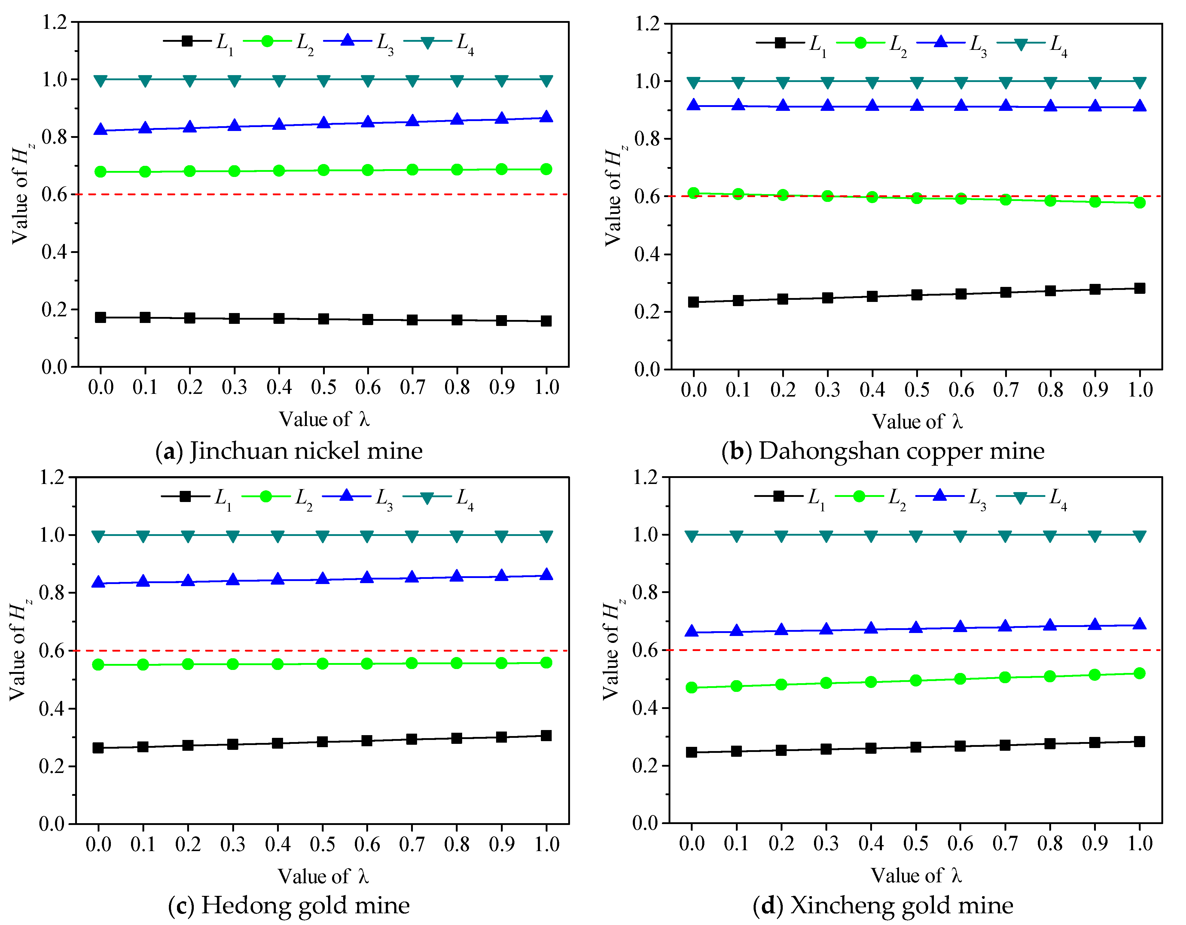
Considering the parameter λ in Equation (10) may affect the evaluation results, it is necessary to explore the effect of different λ values. In this study, the importance of subjective and objective weights is the same, and the value of λ is suggested as 0.5. To confirm the stability of evaluation results, some other λ values are used for comparison. The value of $H_z$ for each mine is shown in Figure 4. It can be seen that the $H_z$ values only change slightly when the λ values alter from 0 to 1. The evaluation results with different λ values are shown in

Table 8. Evaluation results with different λ values.

λ	0	0.1	0.2	0.3	0.4	0.5	0.6	0.7	0.8	0.9	1
Jinchuan nickel mine	$L_2$	$L_2$	$L_2$	$L_2$	$L_2$	$L_2$	$L_2$	$L_2$	$L_2$	$L_2$	$L_2$
Dahongshan copper mine	$L_2$	$L_2$	$L_2$	$L_2$	$L_3$	$L_3$	$L_3$	$L_3$	$L_3$	$L_3$	$L_3$
Hedong gold mine	$L_3$	$L_3$	$L_3$	$L_3$	$L_3$	$L_3$	$L_3$	$L_3$	$L_3$	$L_3$	$L_3$
Xincheng gold mine	$L_3$	$L_3$	$L_3$	$L_3$	$L_3$	$L_3$	$L_3$	$L_3$	$L_3$	$L_3$	$L_3$

. Except for the Dahongshan copper mine, the evaluation results are consistent despite of various λ values. Although the wear risk of Dahongshan copper mine is assessed as $L_2$ when the λ value is 0, 0.1, 0.2 and 0.3, the $H_z$ values are all around 0.6. From a conservative perspective, these risks can also be assessed as $L_3$. It reveals that the proposed methodology has great robustness.

5.2. Comparison Analysis

(1)

Comparison of different connection degree expression

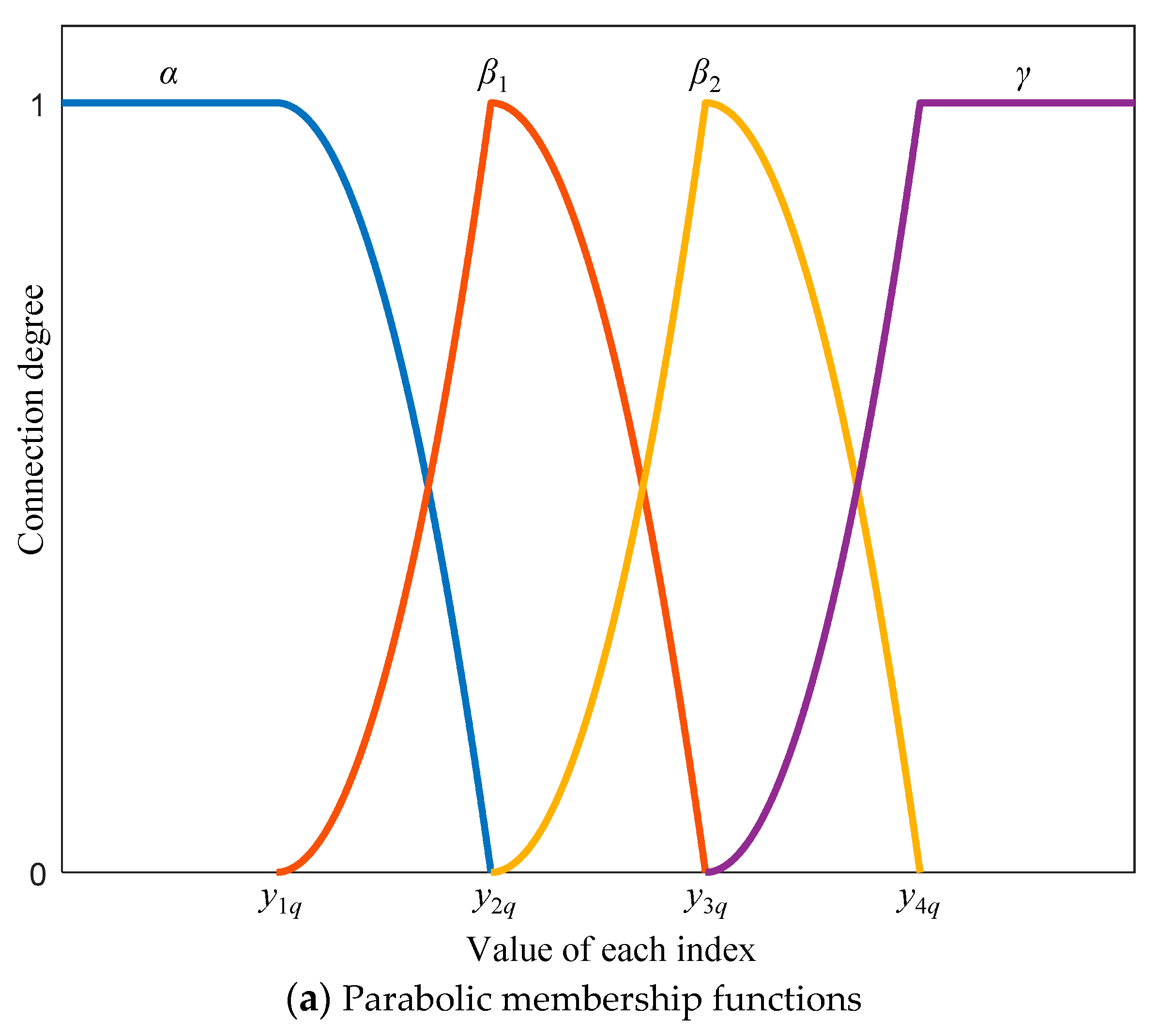
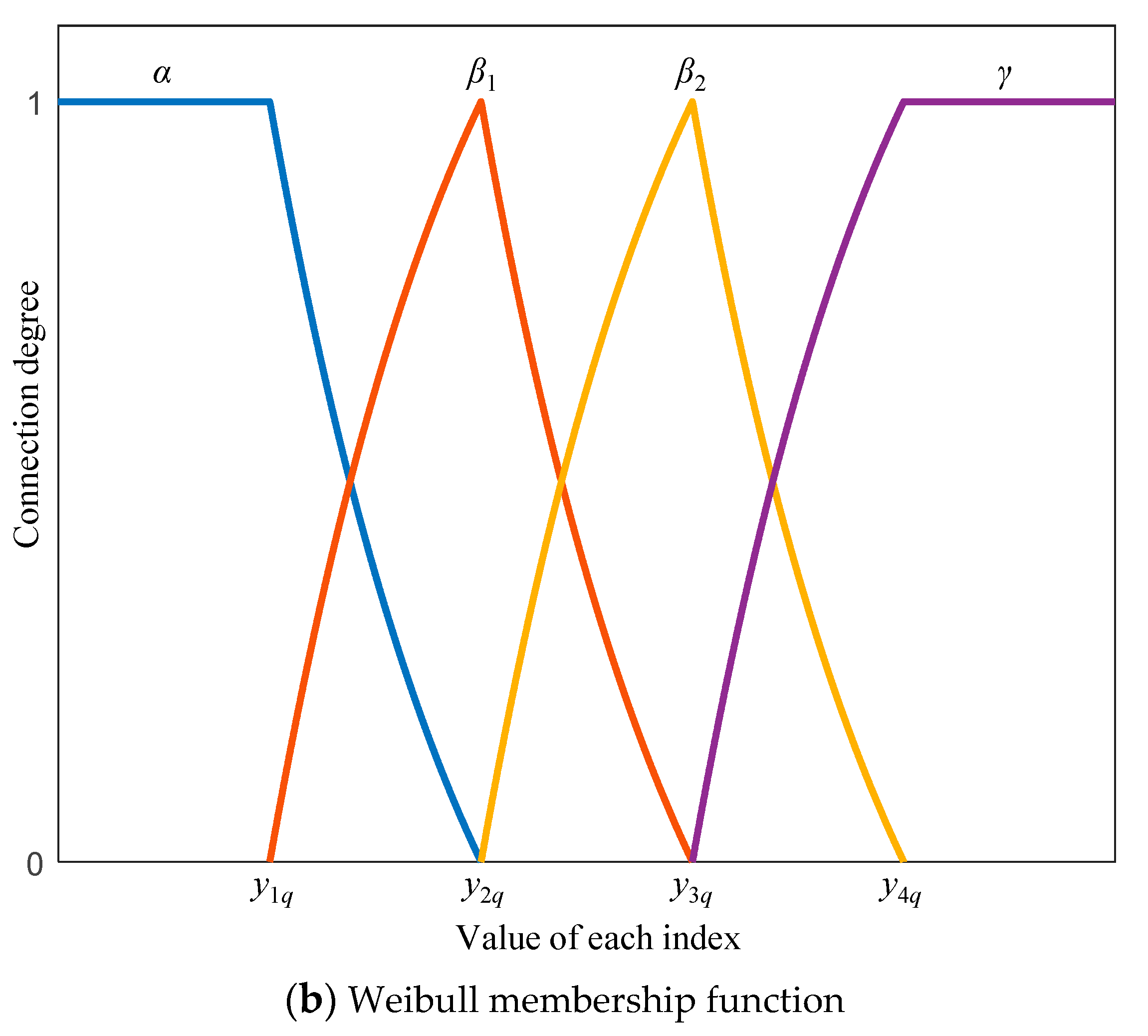
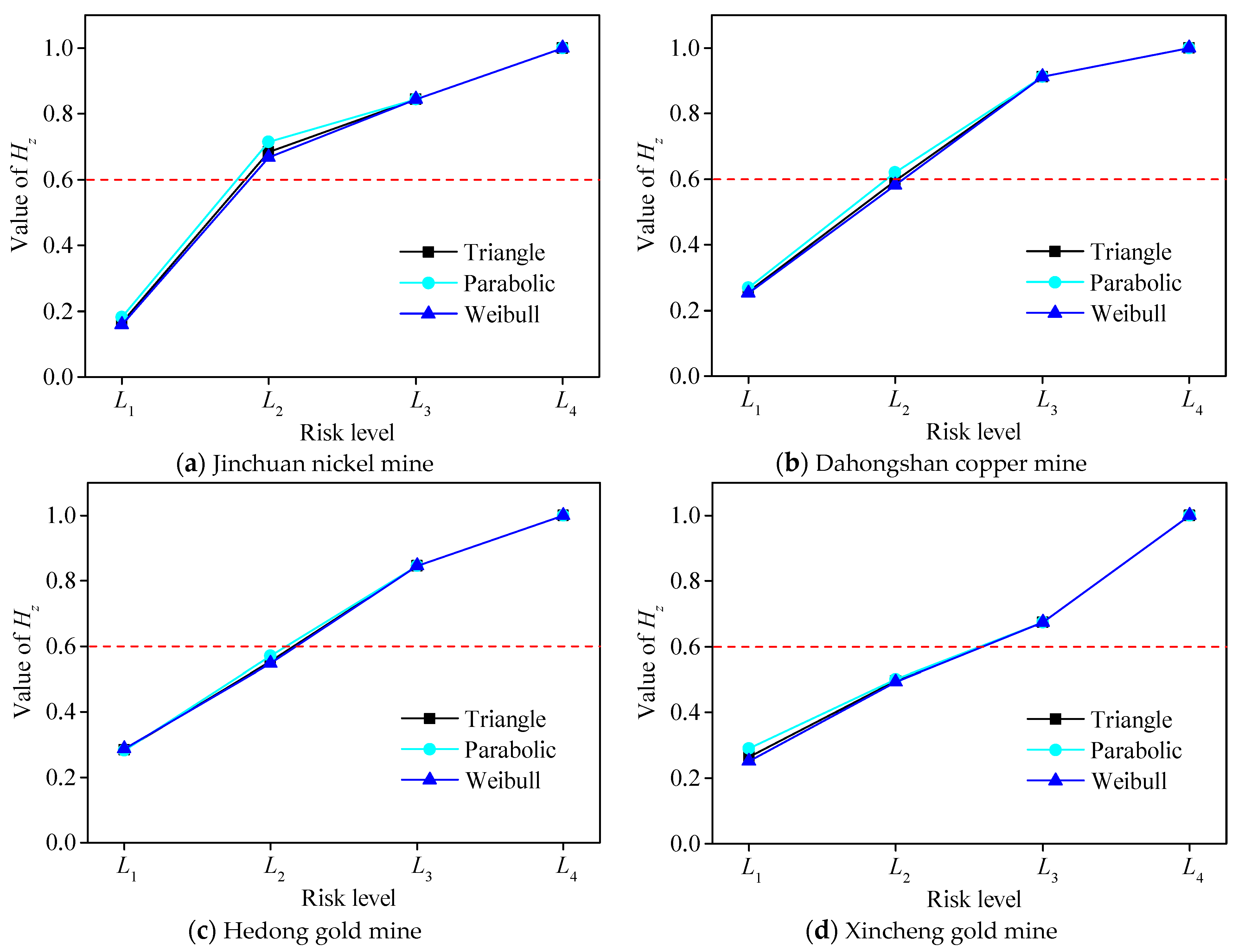
The connection degree has a large influence on evaluation results. In this study, the triangle membership function is selected as the connection degree expression. However, some other forms of membership functions can also be used to determine the connection degree. To analyze the influence of different connection degree expressions, parabolic and Weibull membership functions are used as comparisons [29]. Similar to Figure 3, the schematic diagram of these two connection degree expressions is shown in Figure 5. Then, the value of $H_z$ for each mine is calculated, as shown in Figure 6. It can be seen that the overall difference in the value of $H_z$ is small for these three membership functions. Specifically, the value of $H_2$ for parabolic membership function is slightly larger than that for the other two membership functions. The comprehensive connection degree and risk evaluation results are indicated in

Table 9. Comprehensive connection degree and evaluation results with different membership functions.

Membership Function	Mine	Comprehensive Connection Degree	Risk Level
Parabolic membership function	Jinchuan nickel mine	$\mu =0.1812+0.5338i_1+0.1289i_2+0.1561j$	$L_2$
	Dahongshan copper mine	$\mu =0.2692+0.3519i_1+0.2907i_2+0.0882j$	$L_2$
	Hedong gold mine	$\mu =0.2819+0.2888i_1+0.2750i_2+0.1544j$	$L_3$
	Xincheng gold mine	$\mu =0.2905+0.2101i_1+0.1730i_2+0.3264j$	$L_3$
Weibull membership function	Jinchuan nickel mine	$\mu =0.1593+0.5085i_1+0.1762i_2+0.1561j$	$L_2$
	Dahongshan copper mine	$\mu =0.2520+0.3289i_1+0.3308i_2+0.0882j$	$L_3$
	Hedong gold mine	$\mu =0.2860+0.2611i_1+0.2986i_2+0.1544j$	$L_3$
	Xincheng gold mine	$\mu =0.2512+0.2408i_1+0.1816i_2+0.3264j$	$L_3$

. The evaluation results of all mines are the same when using triangle and Weibull membership functions, while there is only a slight difference for Dahongshan copper mine when using the parabolic membership function. Although the wear risk of Dahongshan copper mine is evaluated as $L_2$, the $H_z$ value is only slightly larger than 0.6. Therefore, the expression of connection degree can affect the results to some extent, but the degree of influence is relatively small in this study.

(2)

Comparison of different confidence levels

The confidence level $\phi$ can influence the final evaluation results directly. In this study, $\phi$ is suggested as 0.6. However, the decision maker may have other preferences. In general, the larger the $\phi$ value, the more conservative the results. Therefore, it is essential to analyze the evaluation results when using different confidence levels. The evaluation results with different confidence levels are shown in

Table 10. Evaluation results with different confidence levels.

Mine	Confidence Level
	$\mathit{\phi }=0.5$	$\mathit{\phi }=0.6$	$\mathit{\phi }=0.7$	$\mathit{\phi }=0.8$	$\mathit{\phi }=0.9$
Jinchuan nickel mine	$L_2$	$L_2$	$L_3$	$L_3$	$L_4$
Dahongshan copper mine	$L_2$	$L_3$	$L_3$	$L_3$	$L_3$
Hedong gold mine	$L_2$	$L_3$	$L_3$	$L_3$	$L_4$
Xincheng gold mine	$L_3$	$L_3$	$L_4$	$L_4$	$L_4$

. It can be seen that the overall risk level increases when the confidence level is higher. In reality, it is not always better when the confidence level is larger. When selecting a higher confidence level, the risk is assessed larger, which means the costs of risk management will be higher. However, if the confidence level is low, the wear risk of backfill pipeline can be underestimated. Therefore, selecting an appropriate confidence level is significant for the wear risk management of backfill pipeline.

In summary, the highlights of this study are as follows:

(1)

The evaluation index system is established from the aspect of slurry characteristics, pipeline properties and slurry flow state, which can fully describe the wear risk of backfill pipeline.

(2)

The extended experts grading method and CRITIC approach are integrated to determine the comprehensive weight, which can simultaneously consider the subjective and objective information.

(3)

The traditional SPA is extended with membership functions and fuzzy entropy theory, which can effectively evaluate the wear risk from both the risk level and complexity.

6. Conclusions

The filling slurry is transported from the surface to the stope through the pipeline system, which inevitably causes the wear of backfill pipeline. This study proposed an extended SPA to evaluate the wear risk of backfill pipeline. In consideration of the wear mechanism of backfill pipeline, the evaluation index system including nine quantitative indexes and three qualitative indexes was established from the aspects of slurry characteristics, pipeline properties, and slurry flow state. The subjective and objective weights were calculated by the extended experts grading method and CRITIC approach, respectively. Then, they were integrated to determine the comprehensive weight. To evaluate the wear risk of backfill pipeline from both the level and complexity, the classical SPA was extended with membership functions and fuzzy entropy theory. The proposed methodology was applied to assess the wear risk in Jinchuan nickel mine, Dahongshan copper mine, Hedong gold mine, and Xincheng gold mine. Results showed that the evaluation results were effective and reliable. Furthermore, the sensitivity analysis indicated that the preference coefficient of weight only had a slight influence on the evaluation results, which revealed the proposed methodology had great stability and robustness. The comparison analysis demonstrated that the expression of connection degree affected the results to some extent, whereas the degree of influence was relatively small in this study. In addition, the confidence level had a great influence on the evaluation results, which depended on the risk appetite of decision makers.

Notably, the specific risk levels were largely dependent on the grading standards and the acceptable confidence level. In the future, it is meaningful to establish a uniform evaluation index system and grading standards. In addition, the proposed methodology can be adopted to solve some similar risk evaluation problems in other engineering fields, such as geotechnical engineering, civil engineering, and environmental engineering.

References

1. Emad, M.Z.; Mitri, H.; Kelly, C. State-of-the-art review of backfill practices for sublevel stoping system. Int. J. Min. Reclam. Environ. 2015, 29, 544–556. [Google Scholar] [CrossRef]
2. Guo, Q.Q.; Yu, H.X.; Dan, Z.Y.; Li, S. Mining Method Optimization of Gently Inclined and Soft Broken Complex Ore Body Based on AHP and TOPSIS: Taking Miao-Ling Gold Mine of China as an Example. Sustainability 2021, 13, 12503. [Google Scholar] [CrossRef]
3. Sivakugan, N.; Veenstra, R.; Naguleswaran, N. Underground mine backfilling in Australia using paste fills and hydraulic fills. Int. J. Geosynth. Ground Eng. 2015, 1, 1–7. [Google Scholar] [CrossRef] [Green Version]
4. Tapsiev, A.P.; Anushenkov, A.N.; Uskov, V.A.; Artemenko, Y.V.; Pliev, B.Z. Development of the long-distance pipeline transport for backfill mixes in terms of Oktyabrsky Mine. J. Min. Sci. 2009, 45, 270–278. [Google Scholar] [CrossRef]
5. Sinha, S.L.; Dewangan, S.K.; Sharma, A. A review on particulate slurry erosive wear of industrial materials: In context with pipeline transportation of mineral-slurry. Part. Sci. Technol. 2017, 35, 103–118. [Google Scholar] [CrossRef]
6. Wang, Y.Y.; Wang, Y.; Yang, G.F.; Ruan, Z.; Wang, Z.Q. Effect of cement-to-tailings ratio and flow rate on the wear performance of filling pipeline. Powder Technol. 2022, 397, 117027. [Google Scholar] [CrossRef]
7. Steward, N.R.; Spearing, A. Combating pipeline wear-an advancing technology. J. S. Afr. Inst. Min. Metall. 1992, 92, 149–157. [Google Scholar]
8. Cooke, R. Pipeline Material Evaluation for the Mina Grande Hydrohoist System. In Proceeding of 13th International Conference on Slurry Handling and Pipeline Transport, Johannesburg, South Africa, 3–5 September 1996; pp. 3–5. [Google Scholar]
9. McGuinness, M.; Cooke, R. Pipeline Wear and the Hydraulic Performance of Pastefill Distribution Systems: The Kidd Mine Experience. In Proceedings of the Minefill 10th International Symposium on Mining with Backfill, Cape Town, South Africa, 21–25 March 2011; The Southern African Institute of Mining and Metallurgy: Johannesburg, South Africa, 2011; pp. 205–212. [Google Scholar]
10. Hewitt, D.; Allard, S.; Radziszewski, P. Pipe lining abrasion testing for paste backfill operations. Miner. Eng. 2009, 22, 1088–1090. [Google Scholar] [CrossRef]
11. Zhang, Q.L.; Cui, J.Q.; Zheng, J.J.; Wang, X.M.; Wang, X.L. Wear mechanism and serious wear position of casing pipe in vertical backfill drill-hole. Trans. Nonferrous Met. Soc. China 2011, 21, 2503–2507. [Google Scholar] [CrossRef]
12. Gharib, N.; Bharathan, B.; Amiri, L.; McGuinness, M.; Hassani, F.P.; Sasmito, A.P. Flow characteristics and wear prediction of Herschel-Bulkley non-Newtonian paste backfill in pipe elbows. Can. J. Chem. Eng. 2017, 95, 1181–1191. [Google Scholar] [CrossRef]
13. Wang, X.L.; Zheng, J.J.; Zhang, Q.L.; Wang, X.M. Influencing factors on the abrasion of pipelines in backfill drilling and protective measures. Min. Metall. Eng. 2009, 29, 9–12. [Google Scholar]
14. Creber, K.J.; Kermani, M.F.; McGuinness, M.; Hassani, F.P. In situ investigation of mine backfill distribution system wear rates in Canadian mines. Int. J. Min. Reclam. Environ. 2017, 31, 426–438. [Google Scholar] [CrossRef]
15. Li, X.C.; Nie, X.X. KPCA-PSO-GRNN evaluation model and application of filling pipeline wear risk. Nonferrous Met. Eng. 2019, 9, 84–92. [Google Scholar]
16. Guo, J.; Zhang, B.X. Invalidation risk evaluation of backfill pipe based on PCA and BP neural network. Gold Sci. Technol. 2015, 23, 66–71. [Google Scholar]
17. Luo, Z.S.; Huang, R.H.; Shen, G.C. Research on wear risk prediction of filling pipeline based on KPCA-IPSO-LSSVM. Gold Sci. Technol. 2021, 29, 245–255. [Google Scholar]
18. Zhang, Q.L.; Hu, W.; Gao, R.W. Analysis of filling pipeline transportation reliability based on extenics. China Saf. Sci. J. 2012, 22, 109–115. [Google Scholar]
19. Xue, X.L.; Wang, X.M.; Zhang, Q.L. An integrated model of combination weights and variable fuzzy on evaluating backfill pipeline wear risk. J. Cent. South Univ. 2016, 47, 3752–3758. [Google Scholar]
20. Wang, S.; Song, X.P.; Shi, H.T. An improved CRITIC and cloud model evaluation method for predicting the wear risk of vertical filling pipes in deep well. J. Chongqing Univ. 2020, 43, 73–84. [Google Scholar]
21. Ding, W.Z.; Shi, X.Z.; Shi, Y. Risk assessment model for wear of backfill pipeline based on improved unascertained measurement. Min. Metall. Eng. 2022, 42, 10–14. [Google Scholar]
22. Guo, E.L.; Zhang, J.Q.; Ren, X.H.; Zhang, Q.; Sun, Z.Y. Integrated risk assessment of flood disaster based on improved set pair analysis and the variable fuzzy set theory in central Liaoning Province, China. Nat. Hazards 2014, 74, 947–965. [Google Scholar] [CrossRef]
23. Chong, T.; Yi, S.; Heng, C. Application of set pair analysis method on occupational hazard of coal mining. Saf. Sci. 2017, 92, 10–16. [Google Scholar] [CrossRef]
24. Roy, D.K.; Datta, B. Adaptive management of coastal aquifers using entropy-set pair analysis–based three-dimensional sequential monitoring network design. J. Hydrol. Eng. 2019, 24, 04018072. [Google Scholar] [CrossRef]
25. Giao, N.T.; Nhien, H.T.H.; Anh, P.K.; Van Ni, D. Classification of water quality in low-lying area in Vietnamese Mekong delta using set pair analysis method and Vietnamese water quality index. Environ. Monit. Assess. 2021, 193, 319. [Google Scholar] [CrossRef] [PubMed]
26. Zhang, L.; Li, H.B. Construction Risk Assessment of Deep Foundation Pit Projects Based on the Projection Pursuit Method and Improved Set Pair Analysis. Appl. Sci. 2022, 12, 1922. [Google Scholar] [CrossRef]
27. Zhao, X.M.; Xu, Z.M.; Sun, Y.Y. Identification of mine water source based on AHP-entropy and set pair analysis. Geofluids 2022, 2022, 3862746. [Google Scholar] [CrossRef]
28. Wang, R.; Zhao, Q.; Sun, H.; Zhang, X.D.; Wang, Y.Y. Risk assessment model based on set pair analysis applied to airport bird strikes. Sustainability 2022, 14, 12877. [Google Scholar] [CrossRef]
29. Zhou, J.; Chen, C.; Wang, M.Z.; Khandelwal, M. Proposing a novel comprehensive evaluation model for the coal burst liability in underground coal mines considering uncertainty factors. Int. J. Min. Sci. Technol. 2021, 31, 799–812. [Google Scholar] [CrossRef]
30. Ding, S.F.; Zhu, H.; Xu, X.Z.; Shi, Z.Z. Entropy-based fuzzy information measures. Chin. J. Comput. 2012, 35, 796–801. [Google Scholar] [CrossRef]
31. Gandhi, B.K.; Borse, S.V. Nominal particle size of multi-sized particulate slurries for evaluation of erosion wear and effect of fine particles. Wear 2004, 257, 73–79. [Google Scholar] [CrossRef]
32. Rong, H.Y.; Peng, Z.J.; Hu, Y.B.; Wang, C.B.; Yue, W.; Fu, Z.Q.; Lin, X.P. Dependence of wear behaviors of hardmetal YG8B on coarse abrasive types and their slurry concentrations. Wear 2011, 271, 1156–1165. [Google Scholar] [CrossRef]
33. Igolkin, A.I.; Zelenin, Y.V. Wear-resistant surfacing on the inner surfaces of pipelines and vessels. Chem. Pet. Eng. 2009, 45, 251–254. [Google Scholar] [CrossRef]
34. Creber, K.J. Experimental and in-situ Investigation into Pipeline Wear in Mine Backfill Distribution Systems. Master’s Thesis, McGill University, Montreal, BC, Canada, 2017. [Google Scholar]
35. Wang, S.; Tang, Y.; Feng, X. Risk assessment of filling pipeline wearing based on improved PCA and ordered multi-class logistic. Gold Sci. Technol. 2019, 27, 740–746. [Google Scholar]
36. Liang, W.Z.; Zhao, G.Y.; Wu, H.; Chen, Y. Assessing the risk degree of goafs by employing hybrid TODIM method under uncertainty. Bull. Eng. Geol. Environ. 2019, 78, 3767–3782. [Google Scholar] [CrossRef]
37. Zhu, Y.J.; Guo, W.; Liu, H.C. Knowledge representation and reasoning with an extended dynamic uncertain causality graph under the Pythagorean uncertain linguistic environment. Appl. Sci. 2022, 12, 4670. [Google Scholar] [CrossRef]
38. Gou, X.J.; Xu, Z.S. Novel basic operational laws for linguistic terms, hesitant fuzzy linguistic term sets and probabilistic linguistic term sets. Inf. Sci. 2016, 372, 407–427. [Google Scholar] [CrossRef]
39. Pang, Q.; Wang, H.; Xu, Z.S. Probabilistic linguistic term sets in multi-attribute group decision making. Inf. Sci. 2016, 369, 128–143. [Google Scholar] [CrossRef]
40. Diakoulaki, D.; Mavrotas, G.; Papayannakis, L. Determining objective weights in multiple criteria problems: The critic method. Comput. Oper. Res. 1995, 22, 763–770. [Google Scholar] [CrossRef]
41. Liu, Y.T.; Zheng, D.J.; Georgakis, C.; Kabel, T.; Cao, E.H.; Wu, X.; Ma, J.J. Deformation analysis of an ultra-high arch dam under different water level conditions based on optimized dynamic panel clustering. Appl. Sci. 2022, 12, 481. [Google Scholar] [CrossRef]
42. Chen, Y.L.; Shen, S.L.; Zhou, A. Assessment of red tide risk by integrating CRITIC weight method, TOPSIS-ASSETS method, and Monte Carlo simulation. Environ. Pollut. 2022, 314, 120254. [Google Scholar] [CrossRef]
43. Xiang, W.Q.; Yang, X.H.; Babuna, P.; Bian, D.H. Development, Application and challenges of set pair analysis in environmental science from 1989 to 2020: A bibliometric review. Sustainability 2021, 14, 153. [Google Scholar] [CrossRef]
Figure 1. Index system for the wear risk evaluation of backfill pipeline.
Sustainability 14 15535 g001
Figure 2. Framework of the proposed methodology.
Sustainability 14 15535 g002
Figure 3. Schematic diagram of connection degree.
Sustainability 14 15535 g003
Figure 4. Value of Hz with different λ values.
Sustainability 14 15535 g004
Figure 5. Diagram of membership functions.
Sustainability 14 15535 g005aSustainability 14 15535 g005b
Figure 6. Value of Hz with different membership functions.
Sustainability 14 15535 g006