Determination of the Parameters of Ground Acoustic-Impedance in Wind Farms

Abstract

The ground surface near a wind turbine has a significant influence on the sound propagation from the turbine, and it is therefore important to determine the ground impedance, a quantity that characterizes the ground surface acoustically. Outdoor ground parameters required by a multi-parameter model used to calculate the ground acoustic-impedance are typically unknown, which brings inconvenience for the model use. This paper introduces a technique to determine the parameters of ground acoustic-impedance for use in a multi-parameter impedance model (for example, the Attenborough four-parameter model). The technique consists of three steps: first, the data for sound-pressure level measured at a distance from two different heights are collected, and the sound-pressure-level difference is calculated; second, in line with the experimental data and the sound-pressure-level calculation formula, the MATLAB optimization tool is used to find the optimal values of the parameters used in the impedance model; and finally, when the optimization is finished, the acoustic impedance of the ground is obtained by substituting the optimal values into the impedance model. To check the performance of the calculation, the calculated sound-pressure-level difference is compared to the experimental one. Compared with a traditional method, the technique can significantly reduce the calculation error.

1. Introduction

Wind-power-generation technology, as one of the most mature renewable energy technologies, has been developed rapidly in recent years to reduce carbon dioxide emissions. As important equipment to convert wind energy, the total installed capacity of a wind turbine is increasing gradually. Although the development of wind power can reduce carbon dioxide emissions, it brings some “contamination—noise pollution, which has become one of the major reasons why some people oppose the development of wind power. The propagation of noise generated by a wind turbine is affected by many factors, including source and receiver heights, distance, atmospheric absorption, wind speed, wind shear, turbulence, temperature, temperature gradient, terrain topography, and so on [1]. Moreover, the normalized ground-impedance, Z, a quantity which characterizes the ground acoustically, also greatly affects the propagation of wind-turbine noise [2]. Consequently, accurately calculating the ground acoustic-impedance in wind farms can help to predict and control wind-turbine noise, so that one can reduce the resistance to wind-energy development.

At present, there are many methods of measuring the ground acoustic-impedance [3,4,5,6,7,8,9,10,11,12,13]. Suárez. et al. [3], for example, evaluated the acoustic impedance of some ground materials commonly found in an urban environment, using different measuring methods. The impedance measurement-methods can be divided into direct methods and indirect methods. The direct methods are the methods to calculate the acoustic impedance directly, without using an acoustic-impedance model. For instance, Allard and Aknine [4] used a free-field two-microphone transfer function to measure acoustic impedance by evaluating sound pressure and normal velocity with a sound-intensity meter. Soh et al. [5] measured the in situ ground acoustic-impedance by measuring the pressure and pressure gradient near a ground for tonal signals. Kirill and Mohamed [6] used standard impedance-tubes to study the effect of water saturation on acoustic impedance. Although direct methods are simple and effective, they are usually used in laboratory environments, which means it is inaccurate for determining the ground acoustic-impedance for the complex terrain on wind farms [7]. Indirect methods are the methods to calculate the ground acoustic-impedance indirectly, by using an acoustic-propagation model and an acoustic-impedance model. Allard and Sieben [8] proposed a method for measuring the acoustic impedance in free field by using two microphones and a spectrum analyzer. In this method, two microphones were set extremely close to the measured ground, and the pressure and sound velocity at the two microphones were measured. The image-source method [2] and the one-parameter acoustic-ground-impedance model of Delany-Bazley [9] were used to fit the parameter of flow resistivity, so as to obtain the ground acoustic-impedance. This method only needs 1 ${\mathrm{m}}^2$ of material to calculate the acoustic impedance of the material. The size of the ground is negligible, since the microphones are very close to the ground, but, due to the small spacing between the two microphones, this method is only suitable for accurate measurements of sound at frequencies above 500 Hz. The Nordtest method [10] is a kind of typical indirect method for measuring the ground acoustic-impedance, which is used to measure in situ the flat outdoor-ground normalized acoustic-impedance by producing a flow-resistivity level; the value can then be used through the impedance model to give a specific acoustic-impedance of the real and imaginary parts, for outdoor sound-propagation calculations. This method is not suitable for calculating the ground acoustic-impedance corresponding to a sound with frequencies below 200 Hz or above 2500 Hz. Recently, Nyborg and Shen [11] introduced a method of determination (original method) that is based on the image-source model and Attenborough’s four-parameter ground acoustic-impedance model [12]. This method is effective for two microphones and one speaker at different distances and heights. The calculated ground acoustic-impedance and flow resistivity are consistent. Since three of the four parameters were estimated according to the information available in the literature, the errors between the computations and measurements were big. In practice, the indirect method is usually based on the Nordtest method or the American National Standards Institute (ANSI) method [10,13] which is a method of deducing the parameter values in an impedance model by fitting the short-range level difference using specified parameters, to calculate the flow-resistivity rate and then obtain the ground acoustic-impedance. To use indirect methods better, there exit various models of calculating the normalized ground-impedance [9,12,14,15,16,17,18,19], categorized with the number of parameters used in the model(s) that characterize the structure of the ground acoustically. Delany and Bazley [9] proposed a one-parameter ground-acoustic-model with flow resistivity, as the parameter has been widely used. Taraldsen and Jonasson [14] derived a new one-parameter model based on the model of Delany and Bazley, for a wider range of applications. Although the one-parameter ground-impedance-model can calculate the surface acoustic-impedance easily, it is not acceptable in physics for not satisfying the condition that the real part of normalized ground-impedance must be greater than zero, even if the ground impedance is modified to satisfy the imaginary part [20]. Compared with one parameter acoustic-impedance models, multi-parameter acoustic-impedance models can better reflect the ground condition. To take the influence of porosity into consideration, Attenborough presented a two-parameter model with porosity and flow resistivity as the parameters [15], which provides a better consistency over low-flow-resistivity grounds such as grasslands. Attenborough also gave a four-parameter model [12], taking flow resistivity ($\sigma$), grain-shape factor ($g$), porosity ($\Omega$) and tortuosity ($s_f$) as the parameters, which is realistic in the multi-parameter model. There are many other acoustic-impedance models, which the reader can find in ref. [16]. In the open air, ground acoustic-parameters, such as porosity, are often unknown and require experimental measurements, which makes the calculation of ground acoustic-impedance difficult. Some researchers proposed models for calculating the ground parameters. Richard and James [21] incorporated the changes in depth in porosity into the equivalent complex-medium Euler equation and continuity equation, and the solution to this wave equation produces meaningful physical results for porosity. Attenborough gave a modified formula for pore-shape-factor ratio in ref. [22] and pore models for different shapes in ref. [12,22,23,24]. However, these models also need some other ground parameters, which makes the calculations complicated. Hence, the required ground-parameters are usually unknown and difficult to measure when multi-parameter models are needed, and usually take empirical values [2,11,16], leading to large errors in the calculation results. Some researchers [25,26] calculated the uncertainty in flow resistivity to be approximately 20–40%.

The purpose of this paper is to present a technique to determine the parameters of ground acoustic-impedance based on the Attenborough four-parameters impedance model [12] and the Shen method [11] to determine the ground acoustic-impedance parameters. As a procedure for solving an optimization problem, an objective function and multiple constraints will be defined. To achieve the optimization result, the fmincon function in Matlab is used.

The paper is organized as follows. In Section 2, the set-up of the experiment and the measured ground are briefly described. In Section 3, the technique for calculating ground acoustic-impedance and an interior-point algorithm is presented. Numerical results and comparisons with field acoustic-measurements are presented in Section 4. Conclusions are drawn in Section 5.

2. Measurement Set-Up

The experimental data used in this paper are from refs. [11,27]. To better understand the measurement data, the experimental set-up and the test ground are briefly described in this section.

As can be seen in Figure 1, Set-up 1 uses one speaker and two microphones. The horizontal distance between the speaker and the microphones is 1.75 m, the height of the speaker is 0.5 m, and the heights of the two microphones are 0.2 m and 0.5 m. Similar to Set-up 1, Set-up 2 also uses one speaker and two microphones, but the distance between the speaker and the microphones is twice that of Set-up 1, i.e., 3.5 m. Accordingly, the heights of the speaker and microphones are doubled to 1 m, 1 m and 0.5 m, respectively.

The specifications and models of speaker and microphones of the two Set-ups are as follows: both set-ups use a Bruel & Kjær omni-source speaker type 4295, which is a mono-directional loudspeaker. The B&K omni-source speaker was connected to an amplifier of Bruel & Kjær Power Amplifier type 2734 in Set-up 1. In Set-up 2, an amplifier of the type orsonic Power Amplifier Nor280 was used, together with the speaker. The measurements required two microphones with a directivity within 1 dB and within ±30°, according to the IEC standard. Two Norsonic Nor1218 microphones, covered with windscreens, were used in both Set-up 1 and Set-up 2.

The uncertainty of the equipment used should be estimated. In the measurement process, the inaccuracies of the microphone heights, speaker height, the horizontal distance, and the equipment error, will affect the accuracy of the measurements. The microphone type used in this case is Norsonic Nor1218, which has an error of ±1 dB according to the IEC standard. Considering that possible measurement errors of height and distance are within ±5%, the maximum error per frequency is 0.48 dB on average using Set-up 1, and 0.66 dB using Set-up 2. According to the Nordtest method [10], to make sure that the sound is only affected by the ground as much as possible, the test-ground-surface unevenness does not exceed ±50 mm, and no vertical reflecting-objects exist at 10 times the distance of separation between the source and the receivers. To minimize the influence of turbulence due to thermal and wind gradients, the wind speed at a height of 1 m above the ground should be less than 5 m/s when carrying out the measurements, and the measurement line should be positioned at the right angle to the wind direction. The heights of the speaker and of the microphones should be measured along the direction normal to the surface of an average ground-plane excluding vegetation. The tests were carried out in an area close to the test turbines at Risø, Denmark. Set up-1 was used in Campaign 1, which were performed on Wednesday May 15, 2019 (Figure 2(left)). The dry ground with freshly cut grass (Ground 1) was for test 1 and the wet ground with freshly cut grass (Ground 2) was for test 2. Campaign 2 was performed on December 4, 2019 (Figure 2(right)) in soft soil ground (Ground 3) (test 3) and wet grassland (Ground 4) (test 4,) where Set-up 2 was used. In the measurements, test signals of both white and pink noise were used with frequencies in the range of 200–2500 HZ in Campaign 1 and 50–2500 HZ in Campaign 2. Each test was repeated four times independently, and in each repeat the set-up was translated to an adjacent ground with no significant changes in geometry. In Campaign 1, each measurement lasted at least 120 s, and 60 s in Campaign 2.

3. Methodology

The Attenborough four-parameter ground acoustic-impedance model [12], the image-source method [2] and the formula for calculating the sound pressure level in the Shen method [11] are used in this study. The optimization algorithm in the MATLAB optimization toolbox is used to find the four parameters corresponding to the minimum error between the calculated and the experimental values. By substituting the obtained four parameters into the Attenborough four-parameter ground-acoustic-model, the surface acoustic-impedance can be calculated with good accuracy.

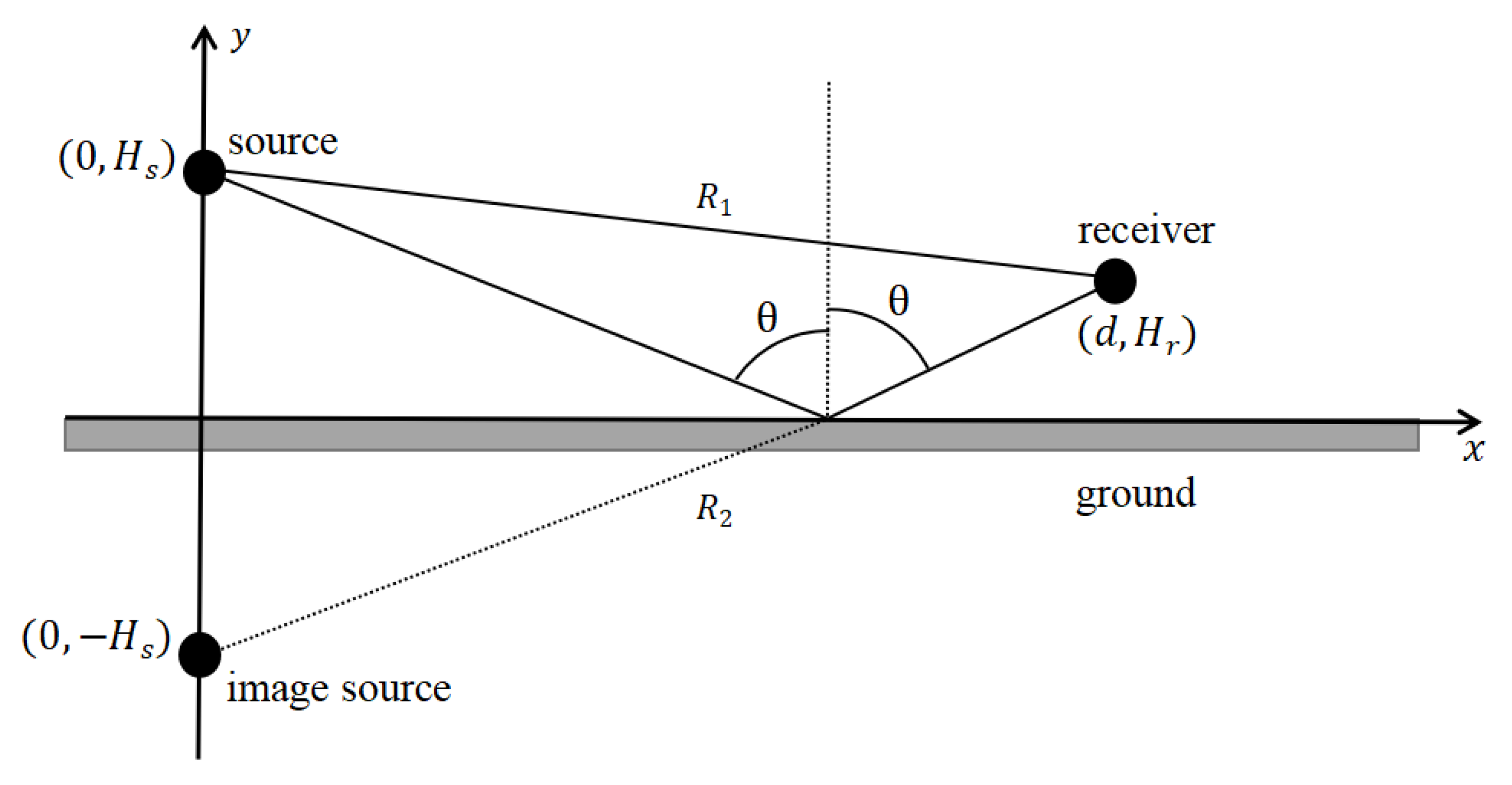
3.1. Image Source Method

When a source and a receiver are close to a ground surface, the calculation of the sound pressure level at the receiver is complex. Due to the reflection of sound by the ground surface, the microphones receive not only the sound directly from the speaker, but also the sound reflected from the ground surface. The interference of the direct and reflected waves has a great influence on the sound field. Because of the phase differences between the direct and the reflect waves, they can interfere with phase-increasing or phase-canceling.

A schematic diagram of the image-source method is shown in Figure 3, where a point source and a receiver are located in a homogeneous atmosphere. With the source and receiver, the x-y coordinate system is set up, with the ground as the x axis, and the y axis perpendicular to the x axis through the sound source; the intersection of the x and y axis is the origin. The source is at the position of (0, $H_s$) and the receiver is at the position of (d, $H_r$). Symmetric with the sound source above the ground, the image source has coordinates of (0, −$H_s$), and the reflection point is where the line between the image source and the receiver intersects at the ground. The angle between the vertical line and the line from the reflection point to the receiver is the reflection angle, which is equal to the incident angle. From the geometry in the figure, the direct distance between the source and the receiver $R_1$, the distance between the image source and the receiver $R_2$, and the reflect angle $\theta ,$ can be calculated easily.

The formula for calculating the sound pressure level at a receiver used by the Shen method in ref. [11] is still applicable in this paper:

$$L_p=S+10log\left(1+\frac{R_1^2}{R_2^2}{\left|Q\right|}^2+\frac{2R_1\left|Q\right|}{R_2}cos\left(k\left(R_2-R_1\right)+\phi \right)\right)-10log\left(4\pi R_1^2\right)$$

(1)

where S is the sound power level of the source, $Q$ is the complex amplitude reflection coefficient of a spherical-wave incident upon a reflecting surface, $k$ is the wave number and $\phi$ is the phase angle between the reflected and the incident rays [27].

Since the sound power level of the source is unknown or not measured, microphones are set up at different heights above the same ground and the sound-pressure-level difference ($\Delta L_P$) of the two microphones is used for the basis of calculation.

$$\Delta L_P=L_{p-top}-L_{p-bottom}$$

(2)

where $L_{p-top}$ is the sound pressure level of the top microphone, and $L_{p-bottom}$ is the sound pressure level of the bottom microphone.

3.2. Four-Parameter Model of Attenborough

To compute the impedance of porous materials, Attenborough developed several refined models, among which the four-parameter model of Attenborough [12] was put into use in this paper:

$$k=\frac{\omega }{c}\sqrt{\gamma \Omega }\sqrt{\left(\frac{4}{3}-\frac{\gamma -1}{\gamma }{N}_{pr}\right)\frac{q^2}{\Omega }+i\frac{s_f^2\sigma }{\rho \omega }}$$

(3)

$$Z=\left(\frac{4q^2}{3\Omega }+i\frac{s_f^2\sigma }{\rho \omega }\right)\frac{\raisebox{1ex}{$\omega $}\!\left/ \!\raisebox{-1ex}{$c$}\right.}{k}$$

(4)

where $\omega =2\pi f$, $c=340 \mathrm{m}/\mathrm{s}$ is the speed of sound, $\gamma =1.4$ is the ratio of specific heats in air, $N_{pr}\approx 0.7$ is the Prandtl number, $\rho =1.2 \mathrm{kg}/{\mathrm{m}}^3$ is the air density, and $q^2={\Omega }^{-g}$. Flow resistivity ($\sigma$), grain-shape factor ($g$), porosity ($\Omega$) and tortuosity ($s_f$) are the four parameters which need to be determined, according to the actual ground situation.

3.3. Technique of Calculating the Ground Acoustic-Impedance

When using the four-parameter model of Attenborough, the other three parameters, except flow resistivity, are typically unknown for outdoor ground surfaces. The measurement of porosity is simple, while the measurements of grain-shape factor and pore-shape-factor ratio are more complex, and it is too cumbersome to measure the porosity every time when calculating an acoustic impedance. As a result, the typical values of the three parameters ($\Omega$ = 0.3, $g$ = 0.5, $s_f=0.75$) were used in the original method [11].

Nevertheless, it is not the value most applicable to the surface of interest, which affects the accuracy of the Attenborough four-parameter ground acoustic-impedance model. In this paper, we introduce an optimization algorithm, with an objective function and four design variables of ($\Omega$, $g$, $s_f$, $\sigma$). To achieve an optimization, the fmincon function in Matlab is used.

To use the fmincon function in Matlab, the initial values should be set first. This paper uses the typical values of the three parameters ($\Omega$ = 0.3, $g$ = 0.5, $s_f=0.75$) as their initial values and uses the Shen method to calculate the flow resistivity as its initial value. In order to apply the algorithm, the range of the four design variables also should also be investigated. The porosity ($\Omega$) of porous materials refers to the ratio of the total volume of pores in porous media to the apparent total volume of materials [28,29]. Saddle-shaped filler and glass fiber have a high porosity, reaching 83~93%. The porosity of coal, concrete, limestone and dolomite can be as low as 2~4%, the porosity of underground sandstone is mostly 12~34%, soil has 43~54%, brick has 12~34%, and leather has 56~59% [30]. In this paper, the ground acoustic-impedance of land and grassland is to be calculated, so the range of porosity is chosen to be 40~60%. The grain-shape factor ($g$) refers to the ratio of the surface area of a sphere to the surface area of a solid particle with the same volume [31]. The grain-shape factor is a dimensionless quantity. Among objects with the same volume but different shapes, the surface area of the sphere shape is the smallest, so the grain-shape factor, $g$, is always less than 1. Since the size of grain-shape factor indicates the degree of difference between the particle shape and the sphere shape, the smaller the shape factor, the longer the shape. If $g$ approaches 1, the grain shape is closer to a sphere, and when $g$ approaches 0, the grain shape tends to be straight or a bar. According to ref. [32], the grain-shape factor of most soil ground and grassland is between 0.5 and 1, so the range of grain-shape factor is chosen to be [0.5, 1]. To introduce the pore-shape-factor ratio, extreme pore shapes are assumed to be circular capillaries with an infinite range of hypotenuse slits, the range of which is [0.6, 1] according to ref. [12]. The Attenborough four-parameters ground acoustic-impedance model was developed for a flow resistivity between 10 and 1000 $\mathrm{kPa}·\mathrm{s}·{\mathrm{m}}^{-2}.$ Since this range is too big, the fmincon function has difficulty finding a suitable value within a reasonable computation time, and thus the search range should be adjusted. The specific process of the range adjustment is shown in Figure 4. The reader is free to adjust the range needed to be obtained in the optimization process.

The range of flow resistivity is determined in the following steps: first, estimate the flow resistivity ($\sigma$) of the ground to be measured. Second, set the first range $\left[\sigma -50\mathrm{kPa}·\mathrm{s}·{\mathrm{m}}^{-2}-2,\sigma +50 \mathrm{kPa}·\mathrm{s}·{\mathrm{m}}^{-2}\right]$ with the estimated value of flow resistance. Third, check the output value: if the output value is within $\left[\sigma -50 \mathrm{kPa}·\mathrm{s}·{\mathrm{m}}^{-2},\sigma -40\mathrm{kPa}·\mathrm{s}·{\mathrm{m}}^{-2}\right]$, then change the range to $\left[\sigma -100\mathrm{kPa}·\mathrm{s}·{\mathrm{m}}^{-2},\sigma \right]$; if the output value is within $\left[\sigma +40 \mathrm{kPa}·\mathrm{s}·{\mathrm{m}}^{-2},\sigma +50 \mathrm{kPa}·\mathrm{s}·{\mathrm{m}}^{-2}\right]$, then change the range to $\left[\sigma ,\sigma +100 \mathrm{kPa}·\mathrm{s}·{\mathrm{m}}^{-2}\right]$; if the output value is equal to the initial value (σ), then change the range to $\left[\sigma +1 \mathrm{kPa}·\mathrm{s}·{\mathrm{m}}^{-2},\sigma +100 \mathrm{kPa}·\mathrm{s}·{\mathrm{m}}^{-2}\right]$ or to $\left[\sigma -100 \mathrm{kPa}·\mathrm{s}·{\mathrm{m}}^{-2},\sigma -1 \mathrm{kPa}·\mathrm{s}·{\mathrm{m}}^{-2}\right]$; otherwise, output the value. Take the middle point in the range as a new σ value, and repeat the steps above. If the minimum error is found with the initial value after changing the range as described previously, the output value is equal to the initial value.

After determining the range of design variables, the fmincon function in MATLAB optimization toolbox is used to find the minimum difference between the calculated and the experimental values, as the goal is to calculate the corresponding four parameters. The fmincon function uses an interior-point algorithm introduced in ref. [33]. When convergence is reached, the obtained values are substituted into the Attenborough four-parameters ground acoustic-impedance model to find the acoustic impedance of the surface.

Moreover, the hybrid shuffled frog-leaping and local search (HSFLA–LS) algorithm proposed in ref. [34], the improved gravitational search algorithm (IGSA) proposed in ref. [35], and the non-parametric kernel density estimation mentioned in ref. [36] can also be used to find the optimal parameter values.

4. Results and Discussions

The technique is applied on the four grounds as described in Section 2. In order to verify the accuracy of the improved method (improved method), this section compares the results of the improved method with those of the Shen method (the original method) and the measured values for white noise and pink noise.

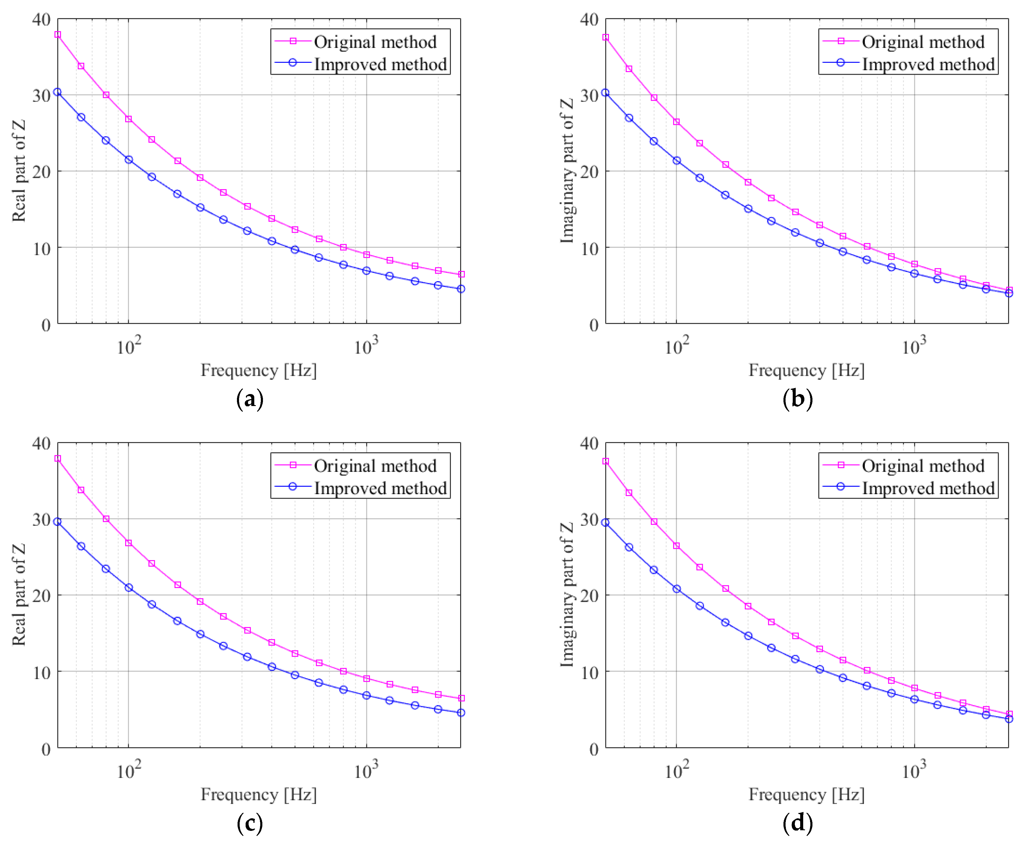
4.1. Calculation of Ground Acoustic-Impedance

In this sub-section, the ground acoustic-impedance and the optimal parameters of the Attenborough four-parameter ground acoustic-impedance model are calculated for a dry and a wet grassland in spring, and a dry grassland and a soil ground in winter. Both the original method and the improved method with the Attenborough four-parameter impedance model are used.

Figure 5 shows the acoustic impedance of the four grounds calculated by using the improved method. The real and imaginary parts of the ground acoustic-impedance decrease when the frequency is increased, and the decreasing speed is slower when the frequency is increased. Additionally, the ground acoustic-impedance is highest in the case of the soil ground in winter, followed by the cases of wet grassland and dry grassland. This is in line with the general law. Moreover, the ground acoustic-impedance of the dry grassland in winter is slightly higher than that in spring, because the grassland is slightly sparse in winter and the soil has a greater influence on the sound. As a conclusion, wind turbines should be erected in dry and vegetated areas.

Table 1. Optimal values of the four parameters for the four grounds obtained by using the improved method.

		Flow Resistivity $\left(\mathit{\sigma }\right)\left[\mathrm{kPa}·s·m^{-2}\right]$	Tortuosity (${\mathit{s}}_{\mathit{f}}$) [-]	Porosity ($\mathit{\Omega }$) [-]	Grain-Shape Factor ($\mathit{g}$) [-]
Ground 1	White noise	257.62	0.7959	0.5417	0.7172
	Pink noise	271.35	0.7666	0.5743	0.6417
Ground 2	White noise	498.75	0.7912	0.5632	0.6782
	Pink noise	501.15	0.8040	0.5619	0.6798
Ground 3	White noise	300.00	0.8289	0.6000	0.5000
	Pink noise	347.15	0.7705	0.6000	0.5000
Ground 4	White noise	853.20	0.8016	0.5121	0.6680
	Pink noise	749.72	0.7931	0.5655	0.7415

shows the optimal values of the four parameters calculated using the improved method for the four land surfaces. Ground 1 is dry grassland in spring, Ground 2 is wet grassland in spring, which is the same ground as Ground 1 but wetted with water, Ground 3 is dry grassland in winter and Ground 4 is soil ground in winter.

As can be seen from the table, the optimal parameters calculated by the improved method for the same ground are almost the same for white noise and pink noise. The flow resistivity of the wet grassland calculated by the improved method is higher than that of the dry grassland, which accords with the general knowledge.

Figure 6, Figure 7, Figure 8 and Figure 9 are the comparisons of the real and imaginary parts of the ground acoustic-impedance for the four grounds, calculated using the improved method and the original method. Ground 1 and Ground 2 were measured at frequencies above 200 Hz and the ground acoustic-impedance was measured at frequencies from 50 to 2500 Hz for Ground 3 and Ground 4 as the distance between the speaker and the microphones was doubled.

As observed, the variation trend of the ground acoustic-impedance calculated using the improved method is similar to that of the original method. Figure 5 shows the surface acoustic-impedance calculated for Ground 1 using the original and the improved methods and two kinds of test noise-sources. For the real part, it can be found that the higher the frequency, the larger the difference between the two methods, and that there exists a relatively smaller difference in the imaginary part. The comparison of the two methods for Ground 2 is shown in Figure 6. Compared with the original method, the real part of the ground acoustic-impedance calculated using the improved method is slightly smaller, and when the frequency is more than 800 Hz, the imaginary parts of the ground acoustic-impedance calculated by the two methods are almost the same. It can be seen in Figure 6 that the differences between the calculated values of ground acoustic-impedance for the two methods are smaller for Ground 3 than for Ground 1 and for Ground 2. As can be seen from Figure 8, the differences in ground acoustic-impedance for Ground 4 calculated using the two methods decrease when the frequency is increased. At high frequencies, the real and imaginary parts of the ground acoustic-impedance obtained by the two methods are almost the same.

It is shown in Figure 5, Figure 6, Figure 7, Figure 8 and Figure 9 that there are some differences between the calculation results of the two methods, but they are within a reasonable range, indicating that the improved method is scientific. The improved method is not simply added to and subtracted from the results of the original method, but is obtained according to the actual ground situation. There is no significant difference between acoustic impedance measured by white noise and pink noise.

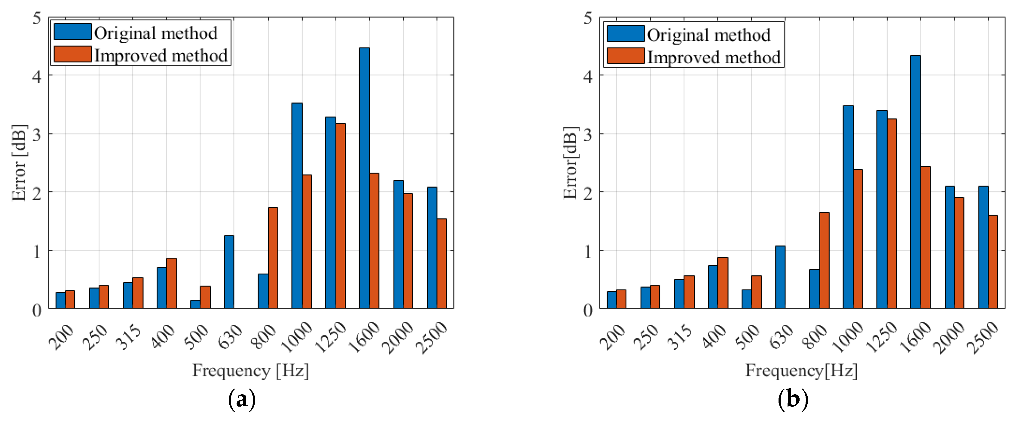
4.2. Accuracy of the Ground Acoustic-Impedance Calculated by the Two Methods

In Section 4.1, the acoustic impedance of the four grounds is calculated using the original method and the improved method, and it is necessary to verify the accuracy of the methods. The ground acoustic-impedance calculated by the two methods is first substituted into Equation (4), the sound pressure level is then calculated using Equation (1), and finally the corresponding sound-pressure-level difference is calculated using Equation (2). The closer the calculated value to the measured value, the more accurate the surface acoustic-impedance.

From Figure 10, Figure 11, Figure 12 and Figure 13, it is seen that both the improved method and the original method are accurate in calculating the surface-acoustic impedance at low frequencies. In the medium frequencies and high frequencies, the improved method agrees much better with the measurement data. In general, the improved method can calculate the surface acoustic-impedance accurately.

As observed, the variation trend of the calculated sound–pressure-level difference with frequency is close to the experimental value. At low frequency, both methods are close to the experimental value, but at medium and high frequency, compared with the original method, the improved method is closer to the experimental value. The improved-method error is reduced by 6–13%, as compared with the original one.

In order to show the errors between the calculated and experimental values more clearly, this paper graphically presents errors ($E_{new}$) between the calculated sound–pressure-level difference obtained using the improved method and the experimental data, and the error ($E_{shen}$) between the original method and the experimental data, in Figure 14, Figure 15, Figure 16 and Figure 17. The unit of error is the decibel [dB].

Figure 14 shows the errors of the improved method and of the original method. It can be seen that both methods agree well with the measurements for frequencies lower than 800 Hz, but the improved method agrees much better with the measurements than the original method for frequencies higher than 1000 Hz. The total errors calculated by the original method using white noise and pink noise for Ground 1 are 15.85 dB and 19.19 dB, respectively, and the total errors of the improved method are 10.94 dB and 10.44 dB for the same ground, which belong to low error according to the Nordtest suggestion, in which they are approximately 5 dB smaller.

It can be seen in Figure 15 that for Ground 2 the improved method and the original method have similar features as Ground 1. The total errors of the original method are 19.43 dB and 19.48 dB for white and pink noise, respectively, and the errors of the improved method are 15.60 dB and 16.81 dB, which are approximately 4 dB smaller.

It is shown in Figure 16 that the differences for Ground 3 are small at medium and low frequencies, but large at high frequencies. At very high frequencies, the error of the improved method is smaller than that of the original method. The errors of the original method measured by white and pink noise are 24.89 dB and 22.99 dB, respectively, and the errors of the improved method are 19.06 dB and 18.04 dB, respectively, which are also approximately 4 dB smaller.

In Ground 4, the errors of the original method are 26.29 dB and 26.83 dB and the errors of the improved method are 24.67 dB and 25.02 dB, which are only 1 dB smaller.

It can be seen from the above figures that, although the original method and the improved method agree well at low frequencies, the errors of the improved method are much lower at high frequencies, and the total errors are greatly reduced. The total errors of the improved method are smaller as compared with those of the original method, no matter what kind of surface it is.

5. Conclusions

In this paper a technique for calculating the acoustic impedance near a wind turbine(s) is developed by modifying the existing Shen method. An optimization algorithm is developed by combining the original method, the Attenborough four-parameter acoustic-impedance model, and the optimization algorithm in the MATLAB toolbox, where the four parameters in the impedance model are used as design variables. Based on the data of sound-pressure-level difference (SPL) measured at Risø, Denmark, the improved method is used to calculate the surface acoustic-impedance. Compared with the original method, the improved method reduces the total errors of the four ground surfaces by 2–5 dB. Compared with the original method using empirical values, the improved method is simple and fast, and can reduce calculation errors, which plays a certain role in promoting the implementation of noise-reduction measures for wind turbines.

References

1. Zeng, M.W.; Zhu, W.J.; Sun, Z.Y.; Zheng, D.Z.; Li, S.L. The influence parameters of aerodynamic noise of wind turbine blades. Appl. Acoust. 2020, 39, 924–931. [Google Scholar]
2. Erik, M.S. Computational Atmospheric Acoustics; Springer: Dordrecht, The Netherlands, 2001; pp. 21–36. [Google Scholar]
3. Suárez, J.G.; Gutiérrez, M.M.; Fernández, A.T.; Lorenzana, T.L.; Arranz, A.M. Comparative Analysis of Several Acoustic Impedance Measurements; Forum Acusticum Sevilla: Sevilla, Spain, 2002. [Google Scholar]
4. Allard, J.F.; Aknine, A. Acoustic impedance measurements with a sound intensity meter. Appl. Acoust. 1985, 18, 69–75. [Google Scholar] [CrossRef]
5. Soh, J.H.; Kenneth, E.G.; Frazier, W.G.; Carrick, L.T.; Roger, W. A direct method for measuring acoustic ground impedance in long-range propagation experiments. J. Acoust. Soc. Am. 2010, 128, 286–293. [Google Scholar] [CrossRef] [PubMed]
6. Kirill, V.H.; Mohamed, H.A.M. Experimental investigation of the effects of water saturation on the acoustic admittance of sandy soils. J. Acoust. Soc. Am. 2006, 120, 1910–1921. [Google Scholar]
7. Kruse, R.; Mellert, V.; Verhey, J.L. In-Situ Measurement of Ground Impedances. Ph.D. Thesis, Technische Universität Braunschweig, Lower Saxony, Germany, 2008. [Google Scholar]
8. Allard, J.F.; Sieben, B. Measurements of acoustic impedance in a free field with two microphones and a spectrum analyzer. J. Acoust. Soc. Am. 1998, 77, 1617. [Google Scholar] [CrossRef]
9. Delany, M.E.; Bazley, E.N. Acoustical properties of fibrous absorbent materials. Appl. Acoust. 1970, 3, 105–116. [Google Scholar] [CrossRef]
10. Nordic Innovation Center. Nordtest Method (NT ACOU 104)—Ground Surfaces: Determination of the Acoustic Impedance. In Teknikantie 12 FIN02150 Espoo Finland; Nordic Innovation Centre: Espoo, Finland, 1999; ISSN 0283-7145. Available online: http://www.nordtest.org (accessed on 8 September 2022).
11. Nyborg, C.M.; Shen, W.Z. New measurement technique for ground acoustic impedance in wind farm. Renew. Energy 2021, 164, 791–803. [Google Scholar] [CrossRef]
12. Attenborough, K. Acoustical impedance models for outdoor ground surfaces. J. Sound Vib. 1985, 99, 521–544. [Google Scholar] [CrossRef]
13. ANSI/ASA S1.18-2010; American National Standard Method for Determining the Acoustic Impedance of Ground Surfaces (Revision of S1.18-1998). American National Standards Institute: New York, NY, USA, 2010.
14. Taraldsen, G.; Jonasson, H. Aspects of ground effect modeling. J. Acoust. Soc. Am. 2011, 129, 47–53. [Google Scholar] [CrossRef] [PubMed]
15. Attenborough, K. Ground parameter information for propagation modeling. J. Acoust. Soc. Am. 1998, 92, 418–427. [Google Scholar] [CrossRef]
16. Attenborough, K.; Bashir, I.; Taherzadeh, S. Outdoor ground impedance models. J. Acoust. Soc. Am. 2011, 129, 2806–2819. [Google Scholar] [CrossRef] [PubMed] [Green Version]
17. Attenborough, K.; Ver, I. Noise and Vibration Control Engineering; Wiley: New York, NY, USA, 2008; pp. 215–278. [Google Scholar]
18. Bérengier, M.C.; Stinson, M.; Daigle, G.A.; Hamet, J.F. Porous road pavements: Acoustical characterization and propagation effects. J. Acoust. Soc. Am. 1997, 101, 155–162. [Google Scholar] [CrossRef]
19. Taraldsen, G. The Delany–Bazley impedance model and Darcy’s Law. Acta Acust. United Acust. 2005, 91, 41–50. [Google Scholar]
20. Dragna, D.; Attenborough, K.; Blanc-Benon, P. On the inadvisability of using single parameter impedance models for representing the acoustical properties of ground surfaces. J. Acoust. Soc. Am. 2015, 138, 2399–2413. [Google Scholar] [CrossRef] [PubMed]
21. Richard, R.; James, M.S. The surface impedance of grounds with exponential porosity profiles. J. Acoust. Soc. Am. 1996, 99, 147–152. [Google Scholar]
22. Attenborough, K. On the acoustic slow wave in air-filled granular media. J. Acoust. Soc. Am. 1987, 81, 93–102. [Google Scholar] [CrossRef]
23. Attenborough, K. Acoustical characteristics of porous materials. Phys. Rep. 1982, 3, 179–227. [Google Scholar] [CrossRef]
24. Attenborough, K. Acoustical characteristics of rigid fibrous absorbents and granular materials. J. Acoust. Soc. Am. 1983, 3, 785–799. [Google Scholar] [CrossRef]
25. Takuya, O.; Masato, T.; Yumi, K. Comparison of flow resistivity values of ground soil obtained by direct measurements and estimations by in-situ acoustic measurements. In Proceedings of the 49th International Congress and Exposition on Noise Control Engineering, Seoul, Republic of Korea, 23 August 2020–26 August 2020; Institute of Noise Control Engineering: Washington, DC, USA, 2020. [Google Scholar]
26. David, E.; Philippe, G.; Benoit, G.; Regis, B.; Hubert, L.; David, L. Uncertainty of an in situ method for measuring ground acoustic impedance. In Proceedings of the 44th International Congress and Exposition on Noise Control Engineering, 44th Inter-Noise Congress, San Francisco, CA, USA, 9 August 2015–12 August 2015. [Google Scholar]
27. Fauri, G. Measurement of the Acoustic Ground Impedance in Wind Farms. Master’s Thesis, Technical University of Denmark, Copenhagen, Denmark, 16 August 2019. [Google Scholar]
28. He, Z.Q.; Yu, M.Z. Method for measuring porosity of porous media. In Proceedings of the Symposium on Construction and Efficient Operation of Heating Engineering, Suzhou, Jiangsu, China, 21 April 2019; pp. 50–56. [Google Scholar]
29. Attenborough, K.; Li, K.M.; Horoshenkov, K. Predicting Outdoor Sound; Taylor & Francis: New York, NY, USA, 2007; pp. 66–109. [Google Scholar]
30. Yang, Q.A. Study on the Flow Characteristics of Particles in Porous Media. Master’s Thesis, Northeast Petroleum University, Daqing, China, 2018. [Google Scholar]
31. Huang, S.P.; Jin, L.; Hu, Z.Q. The influence on Structure and Microstructure of Soil Burned or Roasted from Yang Mausoleum of the Han Dynasty. Chin. J. Soil Sci. 2013, 44, 1337–1342. [Google Scholar]
32. Benjamin, G.Y. The Relationship between the Physical Properties of Soil, Fractal Dimension, and Shape Factors of Its Fragmented Aggregates: A Two-Dimensional Digital Image Processing and Analysis Approach. Ph.D. Thesis, Harbin Institute of Technology, Harbin, China, 2016. [Google Scholar]
33. Nocedal, J.; Öztoprak, F.; Waltz, R.A. An interior point method for nonlinear programming with infeasibility detection capabilities. Optim. Methods Softw. 2014, 29, 837–854. [Google Scholar] [CrossRef]
34. Abdalla, A.N.; Ju, Y.F.; Nazir, M.S.; Tao, H. A Robust Economic Framework for Integrated Energy Systems Based on Hybrid Shuffled Frog-Leaping and Local Search Algorithm. Sustainability 2022, 14, 10660. [Google Scholar] [CrossRef]
35. Nazir, M.S.; Abdalla, A.N.; Zhao, H.Y.; Chu, Z.; Nazir, H.M.J.; Bhutta, M.S.; Javed, M.S.; Sanjeevikumarf, P. Optimized economic operation of energy storage integration using improved gravitational search algorithm and dual stage optimization. J. Energy Storage 2022, 50, 104591–104598. [Google Scholar] [CrossRef]
36. Nazir, M.S.; Abdalla, A.N.; Wang, Y.Q.; Chu, Z.; Jie, J.; Tian, P.; Jiang, M.X.; Jiang, I.; Sanjeevikumar, P.; Tang, Y.F. Optimization configuration of energy storage capacity based on the microgrid reliable output power. J. Energy Storage 2020, 32, 101866–101877. [Google Scholar] [CrossRef]
Figure 1. Schematic diagram of the two Set-ups: (a) Set-up 1, (b) Set-up 2 [11].
Sustainability 14 15489 g001
Figure 2. Selected ground surfaces near a wind turbine [11].
Sustainability 14 15489 g002
Figure 3. Schematic diagram of the image-method principle with a source and a receiver above the ground and an image source below the ground.
Sustainability 14 15489 g003
Figure 4. Flow chart for adjusting the range of flow resistivity.
Sustainability 14 15489 g004
Figure 5. Ground acoustic-impedance of the four grounds at Risø estimated using the improved method. (a) Real part and (b) imaginary part of the ground acoustic-impedance, measured by white noise; (c) real part and (d) imaginary part of the ground acoustic-impedance, measured by pink noise.
Sustainability 14 15489 g005
Figure 6. Real and imaginary parts of the complex ground-impedance for the spring dry grassland at Risø estimated using the original method and the improved method. (a) Real part and (b) imaginary part of ground acoustic-impedance tested with white noise; (c) real part and (d) imaginary part of ground acoustic-impedance tested with pink noise.
Sustainability 14 15489 g006
Figure 7. Real and Imaginary part of the complex ground impedance at the spring wet grassland at Risø estimated using the original method and the improved method. (a) Real part and (b) imaginary part of ground acoustic-impedance tested with white noise; (c) real part and (d) imaginary part of ground acoustic-impedance tested with pink noise.
Sustainability 14 15489 g007
Figure 8. Real and Imaginary part of the complex ground impedance for the winter dry grassland at Risø estimated using the original method and the improved method. (a) Real part and (b) imaginary part of ground acoustic-impedance tested with white noise; (c) real part and (d) imaginary part of ground acoustic-impedance tested with pink noise.
Sustainability 14 15489 g008aSustainability 14 15489 g008b
Figure 9. Real and Imaginary part of the complex ground impedance for the winter soil ground at Risø estimated using the original method and the improved method. (a) Real part and (b) imaginary part of ground acoustic-impedance tested with white noise; (c) real part and (d) imaginary part of ground acoustic-impedance tested with pink noise.
Sustainability 14 15489 g009
Figure 10. SPL difference obtained from the improved method and the original method, together with the four-parameter model and the measurement for the spring dry grassland at Risø. (a) White-noise test signal, (b) pink-noise test signal.
Sustainability 14 15489 g010
Figure 11. Sound-pressure-level (SPL) differences obtained from the improved method and the original method, together with the measurement for the spring wet grassland at Risø. (a) White-noise test signal, (b) pink-noise test signal.
Sustainability 14 15489 g011
Figure 12. SPL difference obtained from the improved method and the original method, together with the measurement for the winter dry grassland at Risø. (a) White-noise test signal, (b) pink-noise test signal.
Sustainability 14 15489 g012
Figure 13. SPL difference obtained from the improved method and the original method, together with the measurement for the winter soil land at Risø. (a) White-noise test signal, (b) pink-noise test signal.
Sustainability 14 15489 g013
Figure 14. Error between the computed and the measured SPL differences of the improved method and the original method with the four-parameter model for the spring dry grassland at Risø (Ground 1). (a) White-noise test signal, (b) pink-noise test signal.
Sustainability 14 15489 g014
Figure 15. Errors between the computed and measured SPL differences obtained from the improved method and the original method with the four-parameter model, for the spring wet grassland at Risø (Ground 2). (a) White-noise test signal, (b) pink-noise test signal.
Sustainability 14 15489 g015
Figure 16. Errors between the computed and measured SPL differences obtained from the improved method and the original method with the four-parameter model, for the winter dry grassland at Risø (Ground 3). (a) White-noise test signal, (b) pink-noise test signal.
Sustainability 14 15489 g016
Figure 17. Errors between the computed and measured SPL differences obtained from the improved method and the original method with the four-parameter model, for the winter soil ground at Risø (Ground 4). (a) White-noise test signal, (b) pink-noise test signal.
Sustainability 14 15489 g017