Article

Optimal Aggregate Size of Traffic Sequence Data Based on Fuzzy Entropy and Mutual Information

1
School of Information and Communication, Guilin University of Electronic Technology, Guilin 541004, China
2
Key Laboratory of Intelligent Traffic System, Guilin University of Electronic Technology, Guilin 541004, China
*
Author to whom correspondence should be addressed.
Sustainability 2022, 14(22), 14767; https://doi.org/10.3390/su142214767
Submission received: 8 September 2022 / Revised: 29 October 2022 / Accepted: 1 November 2022 / Published: 9 November 2022
(This article belongs to the Special Issue Smart Transportation and Intelligent and Connected Driving)

Abstract

:
Before traffic forecasting, it is usually necessary to aggregate the information by a certain length of time. An aggregation size that is too short will make the data unstable and cause the forecast result to be too biased. On the other hand, if the aggregation size is too large, the data information will be lost, resulting in the forecast results tending towards an average or slow response. With the development of intelligent transportation systems, especially the development of urban traffic control systems, high requirements are placed on the real-time accuracy of traffic forecasting. Therefore, it is an essential topic of traffic forecasting research to determine aggregation sizes. In this paper, the mutual information between the forecast input information and the forecast result and the sequence complexity of the forecast result measured by approximate entropy, sample entropy, and fuzzy entropy are considered; then, the optimal data aggregation size is given. To verify the proposed method, the validated data obtained from the simulation is aggregated and calculated with different aggregation sizes, then used for forecasting. By comparing the prediction performance of different aggregate sizes, the optimal aggregate size was found to reduce MSE by 14–30%. The results show that the method proposed in this paper is helpful for selecting the optimal data aggregation size in forecasting and can improve the performance of prediction.

1. Introduction

Short-term traffic forecasting uses past and current traffic information to estimate the future traffic state, such as traffic volume, density, speed, travel demand, and other major traffic parameter characteristics [1]. It has a history of 40 years [2] and has always been an integral part of intelligent transportation systems (ITS) and related research.
In the early stage of the development of short-term traffic forecasting, statistical-based methods were extensively applied to traffic forecasting. These models are usually parametric methods that estimate the model parameters through autoregression and other methods under some reasonable assumptions about the parameters, such as the ARIMA model. Many scholars have improved the autoregressive model in diverse traffic scenarios, such as using a seasonal model to adapt to the periodicity of traffic flow [3], using a heteroscedasticity conditional model to improve the performance of non-stationary traffic forecasting [4,5], and using a cointegration relationship so the forecasting model can be applied in multiple parameter scenarios [6,7]. These measures have improved the performance of the forecasting model in specific scenarios to some extent but also made the model more complex, which makes it difficult for decision-makers to master the model and makes the model more difficult to solve.
As traffic information collection becomes more accessible and computing power increases, many data-driven methods have also been applied to traffic forecasting. These models perform better and are easier to use, such as ensemble learning, neural network methods, and deep learning methods [8,9]. The data-driven methods greatly improve forecast accuracy by fitting a large amount of measured data and can be easily applied to various complex scenarios [10]. Past studies have focused on the study of forecasting methods; trying to obtain higher accuracy. The advent of data mining methods has greatly improved the accuracy of traffic forecasting.
Higher accuracy is the common goal of all traffic forecasting tasks, but it is also necessary to carry out personalized research for diverse traffic prediction tasks. There are many services in the ITS that require technical support for traffic forecasting, such as travel route planning [11], urban traffic management [12], and public transport scheduling [13]. Many services have personalized needs for traffic forecasting, among which the rapid development of UTCS has put forward higher and higher requirements for real-time traffic forecasting [14,15].
UTCS can be divided into three generations based on functions and features [16]. The first generation of UTCS appeared in the 1960s, most of which do not have the data acquisition module and responsiveness [17,18]. SCATS adopts a scheme selection method with partial responsiveness [19]. The second-generation UTCS widely uses the data acquisition module and has the ability to predict traffic, so that the signal control scheme can respond to real-time changes in road traffic conditions [20]. The third generation UTCS puts forward higher requirements for the real-time performance of prediction and its prediction module makes inferences about future road conditions through the spatiotemporal relationship of traffic flow so that it can respond to the foreseeable future traffic state [21].
In each generation of UTCS, traffic forecasting is an indispensable component of the system; with the development of UTCS, its real-time demand for traffic forecasting is getting higher and higher [22,23]. Appropriate data aggregation intervals can reduce the prediction step size, which has an important impact on the real-time performance of predictions. However, blindly reducing the data aggregation interval may result in a loss of prediction accuracy. When the data aggregation size is too small, the collected data contains noise with randomness, which reduces the accuracy of forecast results. However, when the data aggregation size is too large, traffic information will be lost in the aggregation process and the timeliness of forecasting will also be affected due to the increase in forecasting interval [24,25]. UTCS has high requirements for the accuracy and timeliness of traffic forecasting, so the optimization of data aggregation size is crucial to improving the efficiency of UTCS.
In this paper, the optimal data aggregation size is obtained by calculating the mutual information of the forecast inputs and results and the sequence complexity of the forecast results by using approximate entropy, sample entropy, and fuzzy entropy. To validate the proposed method, this paper uses Vissim to simulate the urban traffic environment and collect data. Then, aggregated data of different sizes are used for forecasting and the forecasting performance is compared. The results show that the proposed method is helpful to select the optimal data aggregation size and improve the forecasting performance.
The specific structure of the paper is as follows: Section 1 introduces the definition and calculation method of mutual information. Section 2 introduces three kinds of sequence complexity calculation methods: approximate entropy, sample entropy, and fuzzy entropy. Section 3 designs the Vissim simulation scene and obtains the traffic information required for the forecasting. In Section 4, through the analysis of traffic information, it is found that with the increase of aggregation size, the mutual information increases, and the sequence complexity decreases. A method is proposed to determine the optimal aggregation size by comparing the mutual information corrected using sequence complexity. In Section 5, different aggregation sizes are predicted and the prediction performance is compared and analyzed. Through the comparative analysis of the prediction performance, it is concluded that the proposed optimal aggregation size method can effectively improve the prediction performance.

2. The Measure of Degree of Dependence between Sequences—Mutual Information

To reduce random factors in the data, it is necessary to aggregate the collected data according to a particular time window before traffic forecasting. Aggregation calculation will reduce the randomness of data and make data more stable, but at the same time, it will inevitably lead to the loss of original data. So, an appropriate aggregation size must be selected to protect valid information from being eliminated by aggregation calculation. Mutual information measures the degree of dependence between two pieces of information. In the prediction process, the greater the mutual information between the true value to be predicted and the prediction input, the more related the two are, and the more information can be mined using the prediction model. The quality of different aggregation sizes can be compared by comparing the error between the true value and the predicted result under different aggregation sizes.
Mutual information is a measure used in information theory to evaluate the degree of dependence between two variables. For two random variables, a and b, the mutual information is defined as:
I ( a , b ) = H ( a ) + H ( b ) H ( a , b )
The relationship between mutual information, information entropy, and conditional entropy are shown in Figure 1.
Among them, H(a) and H(b) are the information entropies of random variables a and b. H(a,b) is the joint distribution entropy of a and b. The formula for calculating mutual information can be derived by using Shannon’s information entropy formula.
H ( a ) = a χ p ( a ) l o g ( p ( a ) )
H ( b ) = b ψ p ( b ) l o g ( p ( b ) )
H ( a , b ) = a χ b ψ p ( a , b ) l o g ( p ( a , b ) ) .
According to Formulas (2)–(4), Formula (5) can be obtained:
I ( a , b ) = a χ p ( a ) l o g ( p ( a ) ) b ψ p ( b ) l o g ( p ( b ) ) + a χ b ψ p ( a , b ) l o g ( p ( a , b ) )
= a χ b ψ ( p ( a | b ) p ( b ) l o g   p ( a ) p ( b | a ) p ( a ) l o g   p ( b ) + p ( a , b ) l o g   p ( a , b ) )
= a χ b ψ p ( a , b )   ( l o g   p ( a ) l o g   p ( b ) + l o g   p ( a , b ) ) .
= a χ b ψ p ( a , b )   l o g ( p ( a , b ) p ( a ) p ( b ) )
Mutual information represents the useful information between the predicted and input variables. According to Khinchine’s law of large numbers, as the size of the aggregated sequence increases, the arithmetic mean of the sequence will approach the mathematical expectation, so I(a,b)/H(a) will grow with the increase of the aggregation size. On the other hand, with the increase of the aggregation size, the data will become stable and the diversity and complexity of the sequence will gradually decrease, so some methods are needed to measure the complexity of the sequence.

3. Measure Methods of Sequence Complexity

The traffic system is nonlinear and complex. With the deepening of the research on nonlinear characteristics and chaotic phenomena in traffic flow, more and more dynamic characteristic quantities are used to calculate the complexity of traffic flow, such as Lapunov exponent [26] and power spectrum [27]. However, these calculation methods require long-term stable sequences, which is difficult to suffice in non-stationary traffic flow. A class of sequence information quantitative representation methods represented by approximate entropy has been developed gradually. These methods have a stronger anti-jamming capacity and can judge the complexity of shorter sequences.

3.1. Approximate Entropy

Approximate entropy is a nonlinear dynamic parameter used to quantify the regularity and unpredictability of time series fluctuations. It uses a non-negative number to represent a time series’ complexity [28,29]. Its calculation process is as follows and the corresponding pseudocode is shown in Appendix A:
  • Suppose an n-dimensional time series obtained by sampling at equal time intervals is u(1), u(2), u(3), …, u(N);
  • Define two hyperparameters m and r in the algorithm, where m is an integer greater than or equal to 2, indicating the length of the compared vectors and r is a real number that represents the degree of approximation. The smaller r is, the stricter the algorithm requires on sequence similarity; r generally takes 0.15~0.25;
  • Reconstruct a time series, X(1), X(2), …, X(N + m − 1), where X(i) is vector, equal [u(i), u(I + 1), …, u(I + m − 1)];
  • Pair up any two vectors X(i), X(j) of the reconstructed sequence; I and j are integers in the interval [1, Nm + 1]. Then count the number of vector pairs that satisfy the distance condition. Chebyshev distance is often used here as distance calculation for vectors, that calculation formula is:
    d ( p , q ) = lim k   ( i = 1 n | p i q i | k ) 1 / k = max i ( | p i q i | )
The distance condition is d(X(i), X(j)) ≤ r, so the count of vector pairs that satisfy the condition is:
C r m ( i ) = d [ X ( i ) ,   X ( j ) ] r 1 / ( N m + 1 )
5.
Calculate the average number of paired vectors satisfying the distance condition for each vector:
Φ m ( r ) = i = 1 N m + 1 log ( C r m ( i ) ) / ( N m + 1 )
6.
Calculate the approximate entropy according to the following formula.
A p E n = Φ m ( r ) Φ m + 1 ( r )

3.2. Sample Entropy

Sample entropy is a parameter proposed in 2000 to express the complexity of time series [30,31], which is improved based on approximate entropy. When calculating the vector pair distance, the sample entropy does not include the comparison with its own data segment, which improves the calculation accuracy and reduces the calculation time. In addition, this makes the sample entropy consistent; no matter how the hyperparameter m and hyperparameter r are chosen, more complex sequences always have higher sample entropy. Its calculation process is as follows and the corresponding pseudocode is shown in Appendix A:
1–3.
The first three steps of sample entropy calculation are consistent with the calculation process of approximate entropy;
4.
Counts the number of vector pairs that satisfy the distance condition. The calculation of the sample entropy in this step is similar to the approximate entropy, and the vector distance is also calculated using the Chebyshev distance. However, unlike approximate entropy, the condition of vector pairing not only requires i and j to be any integer in the interval [1, Nm + 1], but also requires to i not be equal to j for sample entropy;
B i m ( r ) = d [ X ( i ) ,   X ( j ) ] r ,   i j 1 / ( N m )
5.
Calculate the average number of paired vectors that satisfy the distance condition for each vector;
Ψ m ( r ) = i = 1 N m B i m ( r ) / ( N m )
6.
Calculate the sample entropy according to the following formula.
S p E n = l n ( Ψ m ( r ) / Ψ m + 1 ( r ) )

3.3. Fuzzy Entropy

Fuzzy entropy is a parameter proposed in 2009 to express the complexity of time series [32], which is further improved based on sample entropy. Fuzzy entropy improves the distance condition using a fuzzy membership function, unlike approximate entropy and sample entropy which take a fixed threshold. Its calculation process is as follows and the corresponding pseudocode is shown in Appendix A:
1–3.
The first three steps of fuzzy entropy calculation are consistent with the calculation process of approximate entropy and sample entropy;
4.
Count the sum of fuzzy memberships of all vector pairs. During the calculation of fuzzy entropy, the vector distance no longer uses the Chebyshev distance and no longer checks whether the vector distance satisfies the distance condition. Instead, calculate the fuzzy membership of each vector pair and sum it up.
A i m ( r ) = j = 1 , j i N = m D m ( i , j ) / ( N m 1 )
where D ( i , j ) = e x p ( ( d ( i , j ) 2 ) r ) , i, and j are integers in the interval [1, Nm + 1], ij;
5.
Calculate the average fuzzy membership for each vector;
Ω m ( r ) = i = 1 N m A i m ( r ) / ( N m )
6.
Calculate the fuzzy entropy according to the following formula.
F u z z y E n = ln ( Ω m ( r ) / Ω m + 1 ( r ) )

4. Simulation to Obtain Experimental Data

This study needs high-resolution sequences that can suffice the requirements of aggregation of different sizes, so the Vissim software is used to simulate the micro-environment of urban traffic to obtain high-resolution data [33,34]. Vissim will collect the time occupancy data of the road at 1S intervals. The simulation scenario of its design is shown below:
Upstream of the detected road segment is a signalized intersection. When random traffic flows through the intersection, it can generate traffic flow that conforms to the characteristics of urban traffic and has some periodicity. After the vehicle leaves the signalized intersection, Vissim will record the data of each vehicle passing 300 m, 600 m, and 900 m downstream of the intersection (D1, D2, D3 in Figure 2).
The signal control scheme of the intersection adopts the fixed scheme, indicating three streams of traffic to enter the detected road segment. (a) The vehicle is controlled by the first signal and goes straight into the detected road segment. (b) The vehicle is controlled by the second signal and turns left into the detected road segment. (c) The vehicle is not constrained by signal control and can freely turn right and enter the detected road segment. The signal lights are displayed in a cycle of 120 s in the order of the light colors as shown in the Figure 3:

5. Calculation of Sequence Information

The road occupancy data obtained from the simulation results obtained by Vissim are aggregated according to a fixed time size m, and the aggregated sequences α m , β m , and χ m of the detectors at D1, D2, and D3 are obtained, respectively. Since there is a time delay in the correlation between the road occupancy at D1 and D2 and D3, the sequence is delayed for n periods, respectively, let B n α m = V m n , B n β m = M m n , and B n χ m = N m n , where B is the lag operator, B n x ( t ) = x ( t n ) .
According to the data detected at D1, D2, and D3, the future data of the road section located at the downstream D1 is predicted, so Formula (8) is used to calculate the mutual information between α m and V m n , α m and M m n , α m and N m n , respectively, to choose the optimal aggregation size and time delay. Taking α m as the predicted result, choosing the delay time n and the aggregation size m when the mutual information is the largest can preserve more details, which is helpful for prediction among different variables.

5.1. Calculation of the Mutual Information of α m and V m n

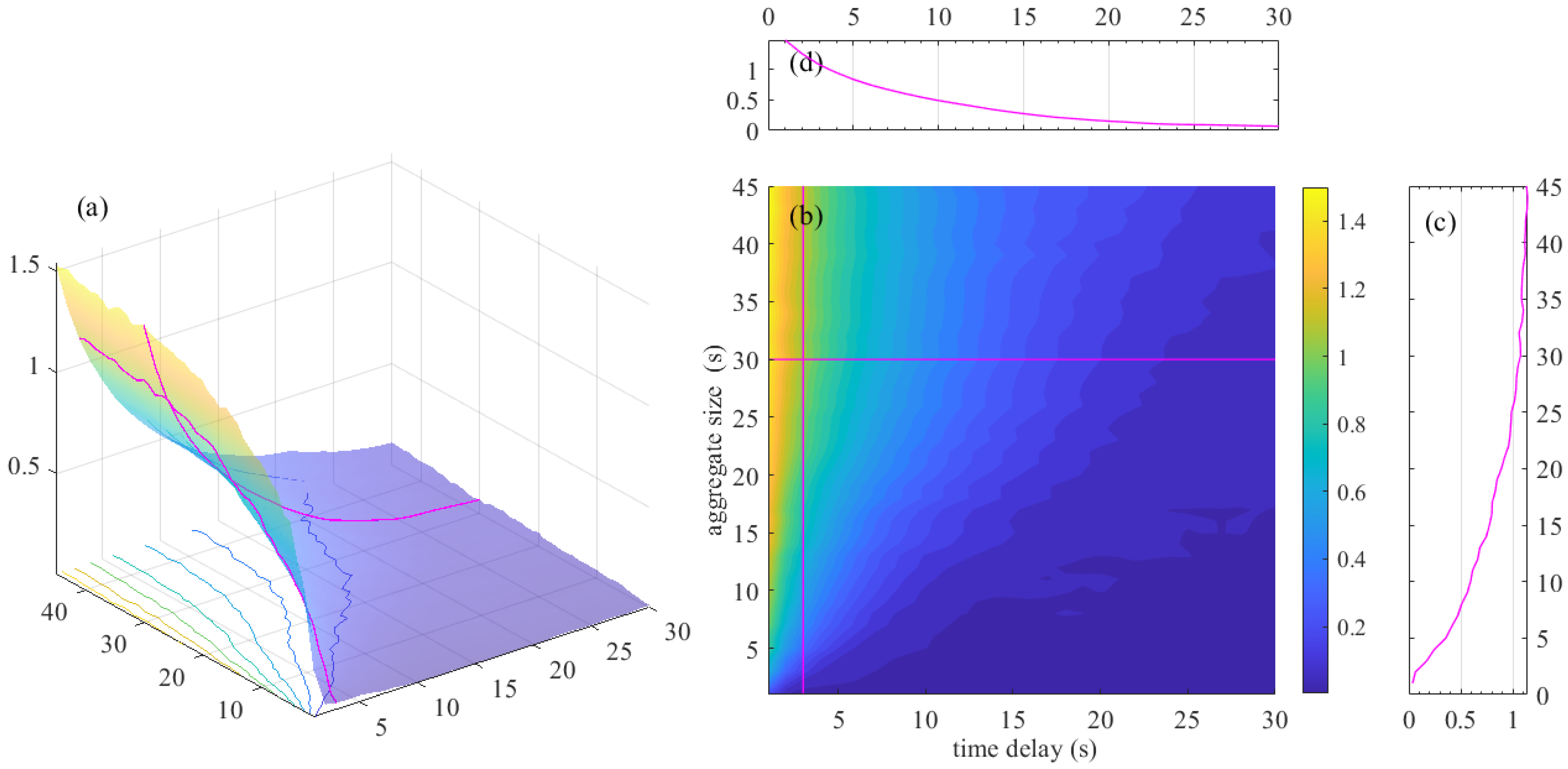
Both α m and V m n sequences originate from the detector D1, so their correlation has no time lag. The mutual information I ( α m , V m n ) was calculated and its distribution along with the aggregation size m and delay time n was drawn in Figure 4, Figure 4a is a 3D distribution graph of mutual information I ( α m , V m n ) distribution; Figure 4b is a heat distribution graph of mutual information I ( α m , V m n ) distribution, Figure 4c shows the variation of mutual information with aggregation size m when the time delay n of V m n is 3, and Figure 4d shows the variation of mutual information with time delay n when the aggregation size m is 30. As the delay time n increases, the mutual information of the two sequences decreases rapidly. On the other hand, as the aggregation size m increases, the road occupancy information tends to be stabler and more average and the mutual information of the two sequences increases.

5.2. Calculation of the Mutual Information of α m and M m n

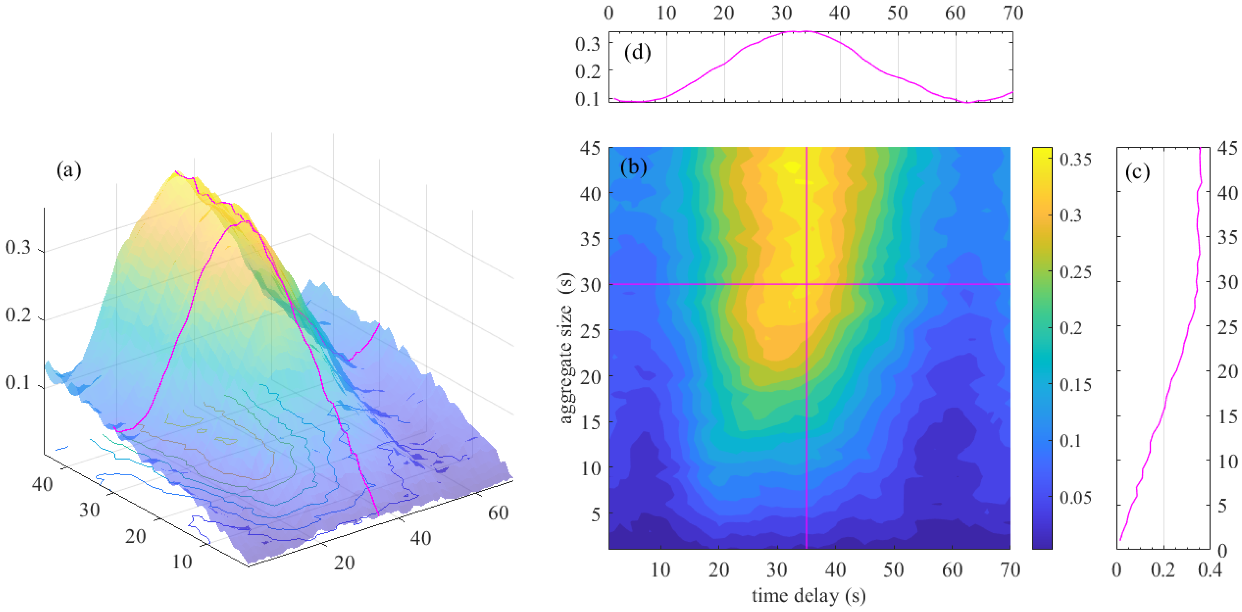
The α m and M m n sequences are collected by the detection points D1 and D2. The two collection points have a spatial distance, so the correlation of the sequences has a time lag. The mutual information I ( α m , M m n ) was calculated and its distribution along with the aggregation size m and delay time n was drawn in Figure 5a as a 3D graph of mutual information I ( α m , M m n ) distribution. Figure 5b is a heat map of mutual information I ( α m , M m n ) distribution. Observing Figure 5a,b, when the delay time is around 35 s, the mutual information is at a high level, so draw Figure 5c to show the change of the mutual information with the aggregation size m when the time delay n is 35. As the aggregation size m increases, the mutual information of the two sequences gradually increases, Figure 5d shows the variation of mutual information with time delay n when the aggregation size m is 30.

5.3. Calculation of the Mutual Information of α m and N m n

The α m and N m n sequences are collected by detection D1 and D3. The two detections have a longer spatial distance, so the time delay of the cross-correlation of the two series is longer. The mutual information I ( α m , N m n ) was calculated and its distribution along with the aggregation size m and delay time n was drawn in Figure 6a as a 3D graph of mutual information I ( α m , N m n ) distribution. Figure 6b is a heat map of mutual information I ( α m , N m n ) distribution. Observing Figure 6a,b, when the delay time is around 65, the mutual information is at a high level, so draw Figure 6c to show the change of the mutual information with the aggregation size m when the time delay n is 65. As the aggregation size m increases, the mutual information of the two sequences gradually increases. Figure 6d shows the variation of mutual information with time delay n when the aggregation size m is 30.

5.4. Calculation of the Complexity of Sequence

The aggregated computation makes the road occupancy information more stable and average; mutual information increases with m. However, the more stable and average road occupancy information contains less information, so the complexity of the sequence α m , β m , and χ m is calculated to measure the information loss caused by the aggregation calculation.
The complexity of the sequence is calculated using approximate entropy, sample entropy, and fuzzy entropy, respectively. In the calculation, the hyperparameters r and m need to be selected, where m is the size of aggregation, the value range is 0–60, r is a parameter that controls the approximate degree of the sequence, and the value is generally recommended to be between 0.2 and 0.3. In this study, r = 0.2, r = 0.25, and r = 0.3 are respectively used for calculation.
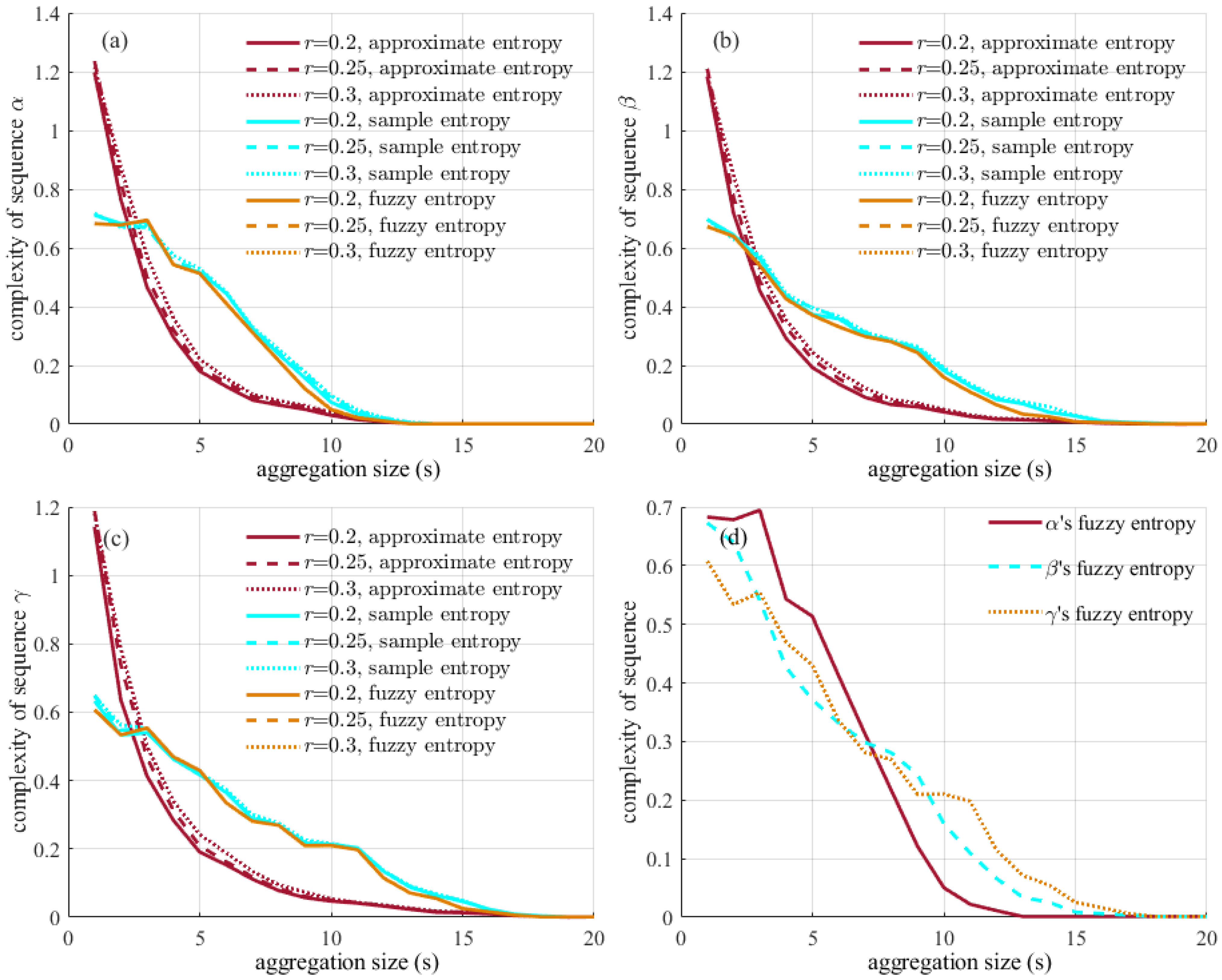
Figure 7a–c all show that the complexity of the sequence declines gradually with the increase of aggregation size m. When m is greater than 15, the road occupancy rate sequence tends toward the average value, which cannot reflect the change of the value in a short time. The choice of parameter r has little influence on the sequence. The fuzzy entropy of sequences α m , β m , and χ m at r = 0.25 is taken for comparison, as shown in Figure 7d. It is observed that the complexity of sequences changes at different speeds with m because the law of platoon dispersion determines that the closer to the intersection, the more complex the sequence. The complexity of α m decreases the fastest, the complexity of β m is the second, and the complexity of χ m is the slowest.

5.5. Select the Optimal Aggregate Size

The mutual information gradually increases with the increase of the aggregation size m and the sequence complexity gradually decreases with the increase of m. The optimal aggregation size m can be found by combining the two indicators so that the predicted sequence contains the most original sequence information. There are many calculation methods for the complexity of the sequence and different hyperparameters can be set. Here, the fuzzy entropy at r = 0.25 is selected as the index to measure the complexity. f u z z y E N ( α m )   I ( α m ,   V m n ) , f u z z y E N ( α m )   I ( α m ,   M m n ) , and f u z z y E N ( α m )   I ( α m ,   N m n ) are calculated, respectively. According to the calculation results, the figures are drawn and then analyzed.
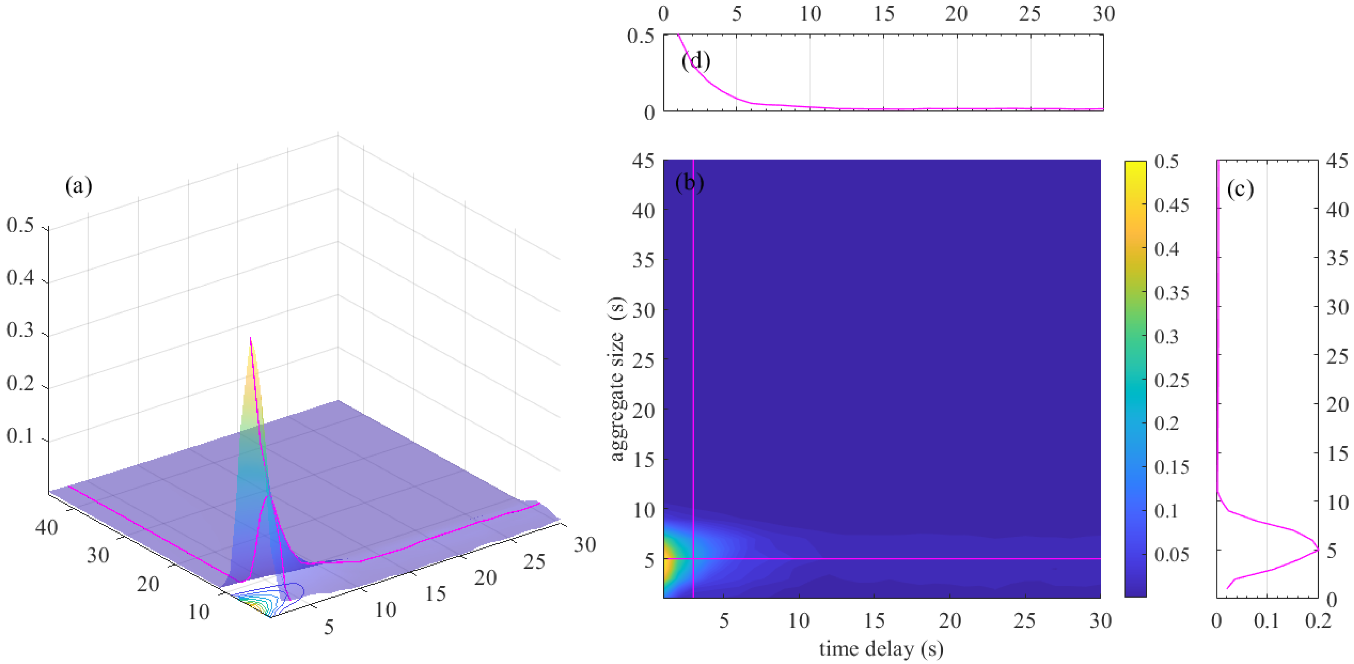
Draw the f u z z y E N ( α m )   I ( α m ,   V m n ) ’s distribution graph as shown in Figure 8. The large value is concentrated in the areas where the time delay is less than 5, and with the increase in the time delay, the amount of information decreases rapidly, which is caused by the autocorrelation of α m . When the aggregation size m is 5, the value is maintained at a high level.
Draw the f u z z y E N ( α m )   I ( α m ,   M m n ) ’s distribution graph as shown in Figure 9. The large value is distributed around the delay time of 20–25 s. Because the detection points D1 and D2 have a spatial distance, there is a time difference between the traffic flow passing through the two detection points in turn, resulting in a time lag cross-correlation (TLCC) between α m and M m n . When the aggregation size is 7, the value is maintained at a high level.
Draw the f u z z y E N ( α m )   I ( α m ,   N m n ) ’s distribution graph as shown in Figure 10. α m and N m n also have a TLCC. When the aggregation size is around 6 and the time delay is around 6, the value remains at a high level.

6. Compare Different Aggregation Sizes

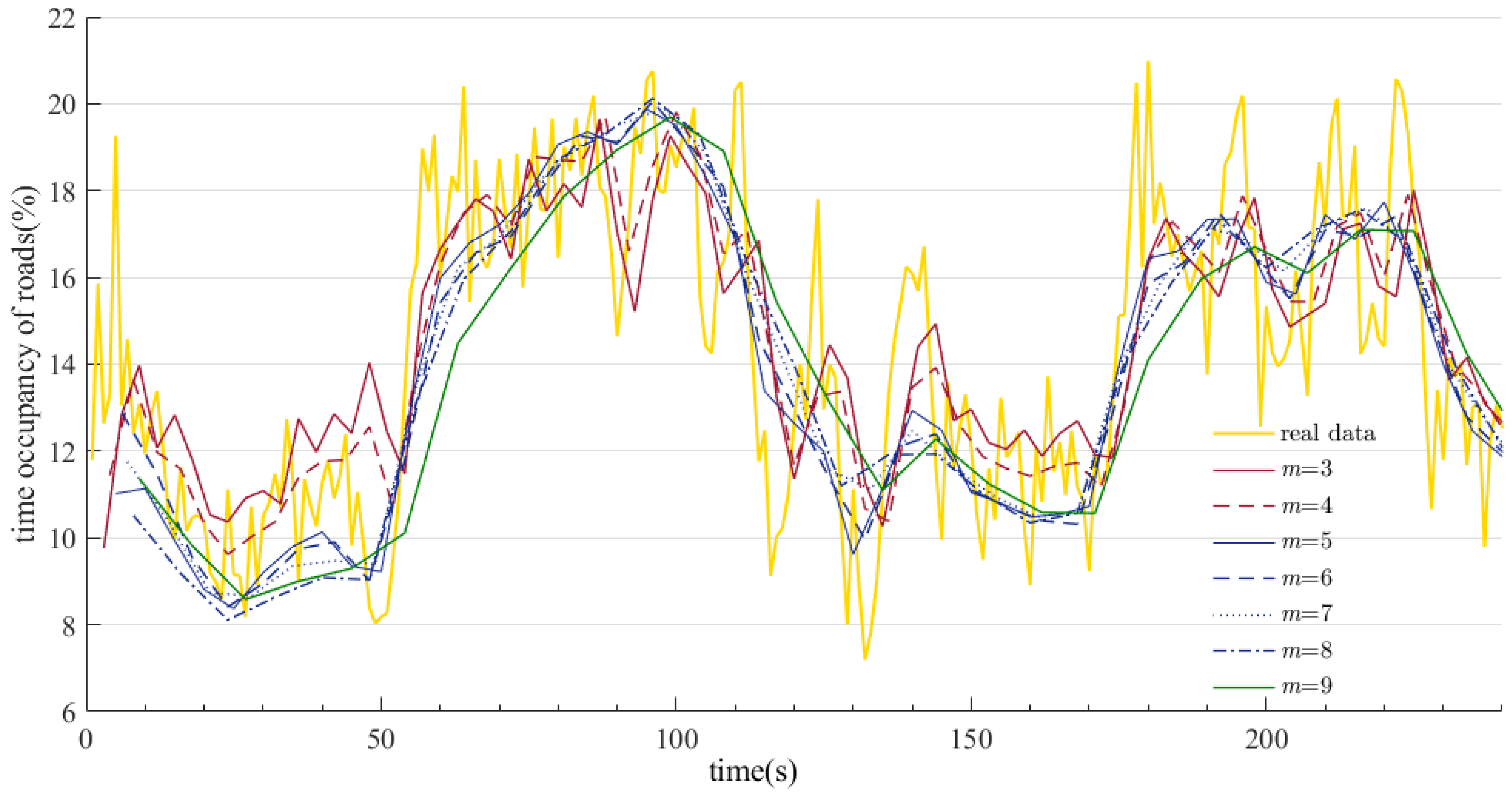
According to the analysis of f u z z y E N ( α m )   I ( α m ,   V m n ) , f u z z y E N ( α m )   I ( α m ,   M m n ) , and f u z z y E N ( α m )   I ( α m ,   N m n ) , aggregation sizes between 5–7 have the highest value. The aggregation size m of the series was respectively set to be 3–9, then the SARIMA method of classical time series analysis was used for prediction. The prediction results are shown in Figure 11 below.
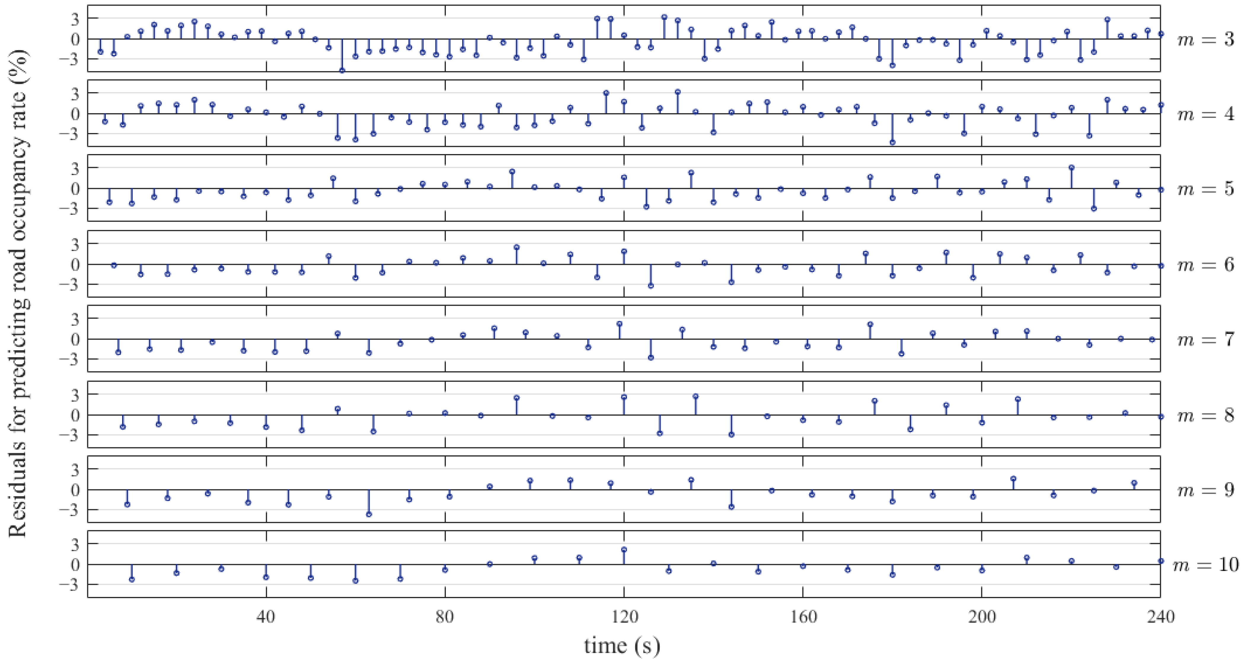
The prediction results of the seven sequences after aggregation can well reflect the real road occupancy rate of the road. In addition, with the increase of aggregation size m, the predicted time occupancy series is gradually smooth and stable but predicted values are more average. To analyze the error distribution of different prediction results, draw the residuals of the predicted time occupancy rate under different aggregation sizes in Figure 12. When the aggregation size is smaller, the error distribution is more concentrated at 0. When the aggregation size m is greater than 5, the maximum residual error of the time occupancy rate can be limited to 3%.
According to the calculation results in Chapter 4, the values of f u z z y E N ( α m )   I ( α m ,   V m n ) , f u z z y E N ( α m )   I ( α m ,   M m n ) , and f u z z y E N ( α m )   I ( α m ,   N m n ) are relatively high when the aggregate size is 5, 6, and 7. At this time, it is considered that the information can be more fully utilized and the prediction performance of UTCS is better. So, the mean MSE of the seven prediction sequences with the times of predictions is plotted in Figure 8a. After about 150 predictions, the mean MSE gradually stabilizes. Figure 13b compares the mean MSE of the seven prediction sequences. When the aggregation size is 5, 6, and 7, the prediction error of road time occupancy is smaller. The predicted MSE when aggregate size is 5, 6, or 7 is approximately 86% of the MSE; when aggregate size is 8, approximately 75% of the MSE when aggregate size is 4; and when aggregate size is 3, approximately 70% of the MSE. This is consistent with the conjecture of the calculation results in Chapter 4, indicating that the method proposed in this paper can select the optimal aggregation size and can significantly reduce the prediction error in UTCS.

7. Conclusions

Choosing an appropriate data aggregation size plays an important role in improving traffic prediction results. This paper proposes a method to select the optimal aggregation size by comparing the mutual information of traffic data with different aggregation sizes and considering the sequence complexity. The experimental data is obtained through Vissim traffic simulation. The analysis of the data shows that the larger the aggregation size, the more stable the sequence and the higher the amount of mutual information. The approximate entropy, sample entropy, and fuzzy entropy are used to calculate the traffic sequence’s complexity. When the data aggregation size is smaller, the content of the traffic sequence is richer. The optimal aggregation size can be obtained by comprehensively considering different aggregation sizes’ mutual information and sequence complexity. The experimental data aggregated with different sizes are predicted, and the prediction performance is compared. The results show that the aggregation size selection method proposed in this paper can help to judge the data aggregation size in traffic prediction, thereby improving the prediction performance in UTCS.

Author Contributions

Conceptualization, J.L.; methodology, J.L.; writing—original draft preparation, J.L.; writing—review and editing, G.L.; visualization, J.L.; supervision, W.L.; project administration, W.L.; funding acquisition, W.L. All authors have read and agreed to the published version of the manuscript.

Funding

This research was funded by the National Natural Science Foundation of China No. 61963011, Guangxi Science and Technology Base and Talent Special Project No. AD19245021, Project of Natural Science Youth Foundation of Guangxi Province No. 2020JJB170049.

Institutional Review Board Statement

Not applicable.

Informed Consent Statement

Not applicable.

Data Availability Statement

Not applicable.

Acknowledgments

We acknowledge the financial support of this research from the relevant grant programs.

Conflicts of Interest

The authors declare no conflict of interest.

Appendix A

Algorithm A1: Calculate the approximate entropy of the sequence
Input:
 U: an array representing an n-dimensional time series sampled at equal time intervals.
 r: a hyperparameter that controls the degree of approximation of the sequence.
 m: aggregation size of the sequence.
Output:
 ApEn: approximate entropy of a sequence.
function ApEnCalculate (U, r, m)  /*main function, calculate approximate entropy*/
1.  A p E n l o g   ( P h i C a l c u l a t e   ( U ,   m ,   r ) / P h i C a l c u l a t e   ( U ,   m + 1 ,   r ) )
2. return  A p E n
end function
function PhiCalculate (U, m, r)  /*subfunction, return the Φ of the reconstructed sequence*/
1.  X [ ]
2. for i in 1 : ( ( l e n g t h   o f   U ) m + 1 )
3.   X [ i ] [ U [ i ] ,   U [ i + 1 ] ,     , U [ i m + 1 ] ]
4. end
5.  C r m [ 0 ,   0 ,   ,   0 ]   1 × l e n g t h   o f   U m + 1
6. foreach i in X
7.  foreach j in X
8.   if Dist (i, j, m) <= r then C r m [ i ] + +
9.  end
10. end
11.  Φ ( C r m ) / ( l e n g t h   o f   U m + 1 )
12. return  Φ
end function
function Dist (a, b, m)  /*subfunction, returns the maximum absolute distance of the input two vectors */
1.  d 0
2. for i in 1:m
3.  if | a ( i ) b ( i ) | > m a x  then  d | a ( i ) b ( i ) |
4. end
5. return max
end function
Algorithm A2: Calculate the sample entropy of the sequence
Input:
 U: an array representing an n-dimensional time series sampled at equal time intervals.
 r: a hyperparameter that controls the degree of approximation of the sequence.
 m: aggregation size of the sequence.
Output:
 SpEn: sample entropy of sequence.
function SpEnCalculate (U, r, m)  /*main function, calculate sample entropy*/
1.  S p E n l o g   ( P s i C a l c u l a t e   ( U ,   m ,   r ) / P s i C a l c u l a t e   ( U ,   m + 1 ,   r ) )
2. return  S p E n
end function
function PsiCalculate (U, m, r)  /*subfunction, return the Ψ of the reconstructed sequence*/
1.  X [ ]
2. for i in 1 : ( ( l e n g t h   o f   U ) m + 1 )
3.   X [ i ] [ U [ i ] ,   U [ i + 1 ] ,     , U [ i m + 1 ] ]
4. end
5.  B r m [   0 ,   0 ,   ,   0   ]   1 × l e n g t h   o f   U m + 1
6. foreach i in X
7.  foreach j in X
8.   if i == j then continue
9.   if Dist (i, j, m) <= r then
10.  end
11. end
12.  Ψ ( B r m ) / ( l e n g t h   o f   U m )
13. return  Ψ
end function
function Dist (a, b, m)  /*subfunction, returns the maximum absolute distance of the input two vectors */
1.  d 0
2. for i in 1:m
3.  if | a ( i ) b ( i ) | > m a x  then  d | a ( i )     b ( i )   |
4. end
5. return d
end function
Algorithm A3: Calculate the fuzzy entropy of the sequence
Input:
 U: an array representing an n-dimensional time series sampled at equal time intervals.
 r: a hyperparameter that controls the degree of approximation of the sequence.
 m: aggregation size of the sequence.
Output:
 FuzzyEn: fuzzy entropy of sequence.
function FuzzyEnCalculate (U, r, m)  /*main function, calculate fuzzy entropy*/
1.  F u z z y E n     l o g   ( O m e g a C a l c u l a t e   ( U ,   m ,   r ) / O m e g a C a l c u l a t e   ( U ,   m + 1 ,   r ) )
2. return  F u z z y E n
end function
function OmegaCalculate (U, m, r)  /*subfunction, return the Ω of the reconstructed sequence*/
1.  X [ ]
2. for i in 1 : ( ( l e n g t h   o f   U ) m + 1 )
3.   X [ i ] [ U [ i ] ,   U [ i + 1 ] ,     , U [ i m + 1 ] ]
4. end
5.  A r m [ 0 ,   0 ,   ,   0 ]   1 × l e n g t h   o f   U m + 1
6. foreach i in X
7.  foreach j in X
8.   if i == j then continue
9.    A r m [   i   ] = e x p   ( D i s t ( i ,   j ,   m ) 2 / r )   /*fuzzy membership function*/
10.  end
11. end
12.  Ω   ( A r m ) / ( l e n g t h   o f   U m )
13. return  Ω
end function
function Dist (a, b, m)  /*subfunction, returns the maximum absolute distance of the input two vectors */
1.  d     0
2. for i in 1:m
3.  if |   a ( i )     b ( i )   |   >   m a x  then  d | a ( i )     b ( i )   |
4. end
5. return d
end function

References

  1. Vlahogianni, E.I.; Golias, J.C.; Karlaftis, M.G. Short-term traffic forecasting: Overview of objectives and methods. Transp. Rev. 2004, 24, 533–557. [Google Scholar] [CrossRef]
  2. Ahmed, M.S.C.; Allen, R. Analysis of freeway traffic time-series data by using Box-Jenkins techniques. Transp. Res. Rec. 1979, 1, 1–9. [Google Scholar]
  3. Wang, Y.; Jia, R.X.; Dai, F.; Ye, Y.X. Traffic Flow Prediction Method Based on Seasonal Characteristics and SARIMA-NAR Model. Appl. Sci. 2022, 12, 2190. [Google Scholar] [CrossRef]
  4. Zhang, Y.R.; Zhang, Y.L.; Haghani, A. A hybrid short-term traffic flow forecasting method based on spectral analysis and statistical volatility model. Transp. Res. Part C Emerg. Technol. 2014, 43, 65–78. [Google Scholar] [CrossRef]
  5. Li, W.Y.; Li, J.Z.; Wang, T. Box-Cox Exponential Transformation. J. Wuhan Univ. Technol. (Transp. Sci. Eng.) 2020, 44, 974–977. [Google Scholar]
  6. Ma, T.; Zhou, Z.; Antoniou, C. Dynamic factor model for network traffic state forecast. Transp. Res. Part B Methodol. 2018, 118, 281–317. [Google Scholar] [CrossRef]
  7. Wang, R.J.; Pei, X.K.; Zhu, J.Y.; Zhang, Z.Y.; Huang, X.; Zhai, J.Y.; Zhang, F.L. Multivariable time series forecasting using model fusion. Inf. Sci. 2022, 585, 262–274. [Google Scholar] [CrossRef]
  8. Inam, S.; Mahmood, A.; Khatoon, S.; Alshamari, M.; Nawaz, N. Multisource Data Integration and Comparative Analysis of Machine Learning Models for On-Street Parking Prediction. Sustainability 2022, 14, 7317. [Google Scholar] [CrossRef]
  9. Li, M.; Li, M.; Liu, B.; Liu, J.; Liu, Z.; Luo, D. Spatio-Temporal Traffic Flow Prediction Based on Coordinated Attention. Sus-tainability 2022, 14, 7394. [Google Scholar] [CrossRef]
  10. Lippi, M.; Bertini, M.; Frasconi, P. Short-Term Traffic Flow Forecasting: An Experimental Comparison of Time-Series Analysis and Supervised Learning. IEEE Trans. Intell. Transp. Syst. 2013, 14, 871–882. [Google Scholar] [CrossRef]
  11. Tettamanti, T.; Demeter, H.; Varga, I. Route Choice Estimation Based on Cellular Signaling Data. Acta Polytech. Hung. 2012, 9, 207–220. [Google Scholar]
  12. Jiang, C.Y.; Hu, X.M.; Chen, W.N. An Urban Traffic Signal Control System Based on Traffic Flow Prediction. In Proceedings of the 2021 13th International Conference on Advanced Computational Intelligence (ICACI), Chongqing, China, 14–16 May 2021; pp. 259–265. [Google Scholar]
  13. Xiao, S. Optimal Travel Path Planning and Real Time Forecast System Based on Ant Colony Algorithm. In Proceedings of the 2017 IEEE 2nd Advanced Information Technology, Electronic and Automation Control Conference (IAEAC), Chongqing, China, 25–26 March 2017; pp. 2223–2226. [Google Scholar]
  14. Balwan, M.A.; Varghese, T.; Nadeera, S. Urban Traffic Control System Review—A Sharjah City Case Study. In Proceedings of the 2021 9th International Conference on Traffic and Logistic Engineering (ICTLE), Macau, China, 9–11 August 2021; pp. 46–50. [Google Scholar]
  15. Woodard, M.; Wisely, M.; Sahra, S.S. A Survey of Data Cleansing Techniques for Cyber-Physical Critical Infrastructure Systems. Adv. Comput. 2016, 102, 63–110. [Google Scholar]
  16. Ghaman, R.; Gettman, D.; Head, L.; Mirchandani, P. Adaptive control software for distributed systems. In Proceedings of the 28th Annual Conference of the IEEE Industrial-Electronics-Society, Seville, Spain, 5–8 November 2002; pp. 3103–3106. [Google Scholar]
  17. Fernandez, R.; Valenzuela, E.; Casanello, F.; Jorquera, C. Evolution of the TRANSYT model in a developing country. Transp. Res. Part A Policy Pract. 2006, 40, 386–398. [Google Scholar] [CrossRef]
  18. Reza, I.; Ratrout, N.T.; Rahman, S.M. Artificial Intelligence-Based Protocol for Macroscopic Traffic Simulation Model Development. Arab. J. Sci. Eng. 2021, 46, 4941–4949. [Google Scholar] [CrossRef]
  19. Tian, Z.; Ohene, F.; Hu, P.F. Arterial Performance Evaluation on an Adaptive Traffic Signal Control System. Procedia Soc. Behav. Sci. 2011, 16, 230–239. [Google Scholar] [CrossRef] [Green Version]
  20. Dusparic, I.; Monteil, J.; Cahill, V. Towards Autonomic Urban Traffic Control with Collaborative Multi-Policy Reinforcement Learning. In Proceedings of the 2016 IEEE 19th International Conference on Intelligent Transportation Systems (ITSC), Rio de Janeiro, Brazil, 1–4 November 2016; pp. 2065–2070. [Google Scholar]
  21. Mirchandani, P.; Wang, F.Y. Rhodes to Intelligent Transportation Systems. IEEE Intell. Syst. 2005, 20, 10–15. [Google Scholar] [CrossRef]
  22. Moharm, K.I.; Zidane, E.F.; El-Mahdy, M.M.; El-Tantawy, S. Big Data in ITS: Concept, Case Studies, Opportunities, and Challenges. IEEE Trans. Intell. Transp. Syst. 2019, 20, 3189–3194. [Google Scholar] [CrossRef]
  23. Shengdong, M.; Zhengxian, X.; Yixiang, T. Intelligent Traffic Control System Based on Cloud Computing and Big Data Mining. IEEE Trans. Ind. Inform. 2019, 15, 6583–6592. [Google Scholar] [CrossRef]
  24. Suvin, P.V.; Karmakar, A.R.; Islam, S.Y.; Mallikarjuna, C. Criteria for Temporal Aggregation of the Traffic Data from a Heterogeneous Traffic Stream. Transp. Res. Procedia 2020, 48, 3401–3412. [Google Scholar] [CrossRef]
  25. Weerasekera, R.; Sridharan, M.; Ranjitkar, P. Implications of Spatiotemporal Data Aggregation on Short-Term Traffic Pre-diction Using Machine Learning Algorithms. J. Adv. Transp. 2020, 2020, 1–21. [Google Scholar] [CrossRef]
  26. Liu, Y.; Zhang, J.Z. Predicting Traffic Flow in Local Area Networks by the Largest Lyapunov Exponent. Entropy 2016, 18, 32. [Google Scholar] [CrossRef] [Green Version]
  27. Chen, Y.Y.; Lv, Y.S. Analysis and Forecasting of Urban Traffic Condition Based on Categorical Data. In Proceedings of the 2016 IEEE International Conference on Service Operations and Logistics, and Informatics (Soli), Beijing, China, 10–12 July 2016; pp. 113–118. [Google Scholar]
  28. Pincus, S.M. Approximate Entropy as a Measure of System-Complexity. Proc. Natl. Acad. Sci. USA 1991, 88, 2297–2301. [Google Scholar] [CrossRef] [PubMed] [Green Version]
  29. Li, Z.; Cai, J.P.; Lu, X.F.; Si, J.B. Complexity Measure of FH/SS Sequences Using Approximate Entropy. In Proceedings of the 2009 IEEE International Conference on Communications, Dresden, Germany, 14–18 June 2009; pp. 834–838. [Google Scholar]
  30. Richman, J.S.; Moorman, J.R. Physiological time-series analysis using approximate entropy and sample entropy. Am. J. Physiol. Heart Circ. Physiol. 2000, 278, H2039–H2049. [Google Scholar] [CrossRef] [PubMed] [Green Version]
  31. Delgado-Bonal, A.; Marshak, A. Approximate Entropy and Sample Entropy: A Comprehensive Tutorial. Entropy 2019, 21, 541. [Google Scholar] [CrossRef]
  32. Chen, W.T.; Zhuang, J.; Yu, W.X.; Wang, Z.Z. Measuring complexity using FuzzyEn, ApEn, and SampEn. Med Eng. Phys. 2009, 31, 61–68. [Google Scholar] [CrossRef]
  33. Krivda, V.; Petru, J.; Macha, D.; Novak, J. Use of Microsimulation Traffic Models as Means for Ensuring Public Transport Sustainability and Accessibility. Sustainability 2021, 13, 2709. [Google Scholar] [CrossRef]
  34. Alrukaibi, F.; Alsaleh, R.; Sayed, T. Applying Machine Learning and Statistical Approaches for Travel Time Estimation in Partial Network Coverage. Sustainability 2019, 11, 3822. [Google Scholar] [CrossRef]
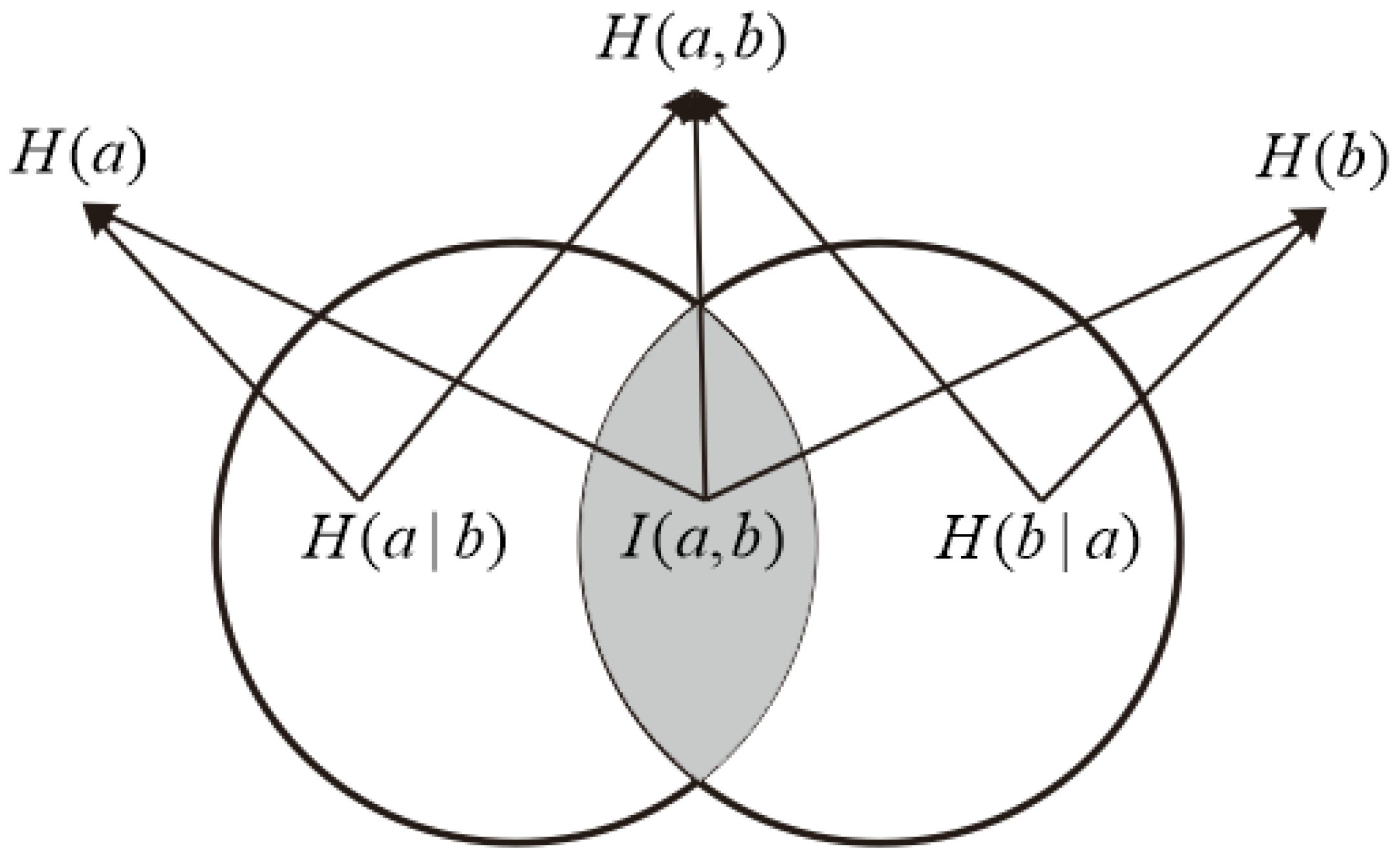
Figure 1. An overview of mutual information.
Sustainability 14 14767 g001
Figure 2. Overview diagram of simulation.
Sustainability 14 14767 g002
Figure 3. The signal control scheme in the simulation scenario.
Sustainability 14 14767 g003
Figure 4. Distribution of the mutual information of α m and V m n , in different aggregation sizes and delay: (a) Mutual information’s 3D distribution graph. (b) Mutual information’s heat distribution graph. (c) Mutual information’s distribution graph when n = 3. (d) Mutual information’s distribution graph when m = 30.
Sustainability 14 14767 g004
Figure 5. Distribution of the mutual information of α m and M m n , in different aggregation sizes and delay: (a) Mutual information’s 3D distribution graph. (b) Mutual information’s heat distribution graph. (c) Mutual information’s distribution graph when n = 35. (d) Mutual information distribution graph when m = 30.
Sustainability 14 14767 g005
Figure 6. Distribution of the mutual information of α m and N m n , in different aggregation sizes and delay: (a) Mutual information’s 3D distribution graph. (b) Mutual information’s heat distribution graph. (c) Mutual information’s distribution graph when n = 65. (d) Mutual information’s distribution graph when m = 30.
Sustainability 14 14767 g006
Figure 7. The complexity of α m , β m , and χ m : (a) Approximate entropy, sample entropy, and fuzzy of α m . (b) Approximate entropy, sample entropy, and fuzzy of β m . (c) Approximate entropy, sample entropy, and fuzzy of χ m . (d) α m ’s, β m ’s, and χ m ’s fuzzy entropy, when r is 0.25.
Sustainability 14 14767 g007
Figure 8. Distribution of f u z z y E N ( α m )   I ( α m ,   V m n ) in different aggregation sizes and delay. (a) 3D distribution graph of f u z z y E N ( α m )   I ( α m ,   V m n ) . (b) Heat distribution graph of f u z z y E N ( α m )   I ( α m ,   V m n ) . (c) Distribution graph of f u z z y E N ( α m )   I ( α m ,   V m n ) , when n = 3; (d) Distribution graph of f u z z y E N ( α m )   I ( α m ,   V m n ) , when m = 5.
Sustainability 14 14767 g008
Figure 9. Distribution of f u z z y E N ( α m )   I ( α m ,   M m n ) in different aggregation sizes and delay. (a) 3D distribution graph of f u z z y E N ( α m )   I ( α m ,   M m n ) . (b) Heat distribution graph of f u z z y E N ( α m )   I ( α m ,   M m n ) . (c) Distribution graph of f u z z y E N ( α m )   I ( α m ,   M m n ) , when n = 20. (d) Distribution graph of f u z z y E N ( α m )   I ( α m ,   M m n ) , when m = 7.
Sustainability 14 14767 g009
Figure 10. Distribution of f u z z y E N ( α m )   I ( α m ,   N m n ) in different aggregation sizes and delay. (a) 3D distribution graph of f u z z y E N ( α m )   I ( α m ,   N m n ) . (b) Heat distribution graph of f u z z y E N ( α m )   I ( α m ,   N m n ) . (c) Distribution graph of f u z z y E N ( α m )   I ( α m ,   N m n ) , when n = 60. (d) Distribution graph of f u z z y E N ( α m )   I ( α m ,   N m n ) , when m = 6.
Sustainability 14 14767 g010
Figure 11. Prediction results for different aggregation sizes.
Sustainability 14 14767 g011
Figure 12. Prediction error at different aggregation sizes.
Sustainability 14 14767 g012
Figure 13. MSE for road occupancy rate predictions with different aggregation sizes: (a) The mean MSE becomes stable with the increase of prediction’s count. (b) Comparison of mean MSE for different aggregate sizes when prediction’s count is 240.
Sustainability 14 14767 g013
Publisher’s Note: MDPI stays neutral with regard to jurisdictional claims in published maps and institutional affiliations.