Article

The Influencing Mechanisms on Global Industrial Value Chains Embedded in Trade Implied Carbon Emissions from a Higher-Order Networks Perspective

School of Economics, Hebei GEO University, Shijiazhuang 050031, China
*
Author to whom correspondence should be addressed.
Sustainability 2022, 14(22), 15138; https://doi.org/10.3390/su142215138
Submission received: 10 October 2022 / Revised: 9 November 2022 / Accepted: 11 November 2022 / Published: 15 November 2022

Abstract

:
As the division of labor in global industrial value chains deepens, the embedded relationships and carbon emission relationships among countries become more complex. First, calculate the embedding indices of forward and backward global industrial value chains and establish the Multi-Regional Input Output (MRIO) model to calculate trade-implied carbon emissions. Second, construct higher-order weighted networks characterized by hypergraphs from 2000 to 2018, and calculate a high-dimensional vector of characteristic indicators based on apices and hyperedges. Finally, time exponential random graph models are constructed using maximum pseudo-likelihood estimation and Markov Monte Carlo simulation methods to dynamically observe the evolution of the impact mechanism of forward and backward industrial value chains embedded in trade-implied carbon emissions networks. The conclusions obtained are as follows: First, most countries tend to develop backward industries when embedded in global industrial value chains. Second, based on the Global Industry Classification Standard (GICS) criteria, industries deeply embedded in global forward value chains are mainly concentrated in materials and utilities, etc., while industries more deeply embedded in global backward value chains are mainly concentrated in consumer discretionary and real estate industries, etc. Third, “carbon transfer” and “carbon leakage” gradually widen the gap between developed and developing countries, both on the production and consumption sides. Fourth, we decompose the factors influencing industrial carbon emissions into carbon intensity effects, industrial structure effects, and output scale effects and analyze their influence mechanisms. Fifth, for countries with different carbon flow attributes, their forward and backward embedded global industrial value chains have different effects on trade-implied carbon emissions. Sixth, the effective paths of trade that lead to a reduction in carbon emissions are different for countries with different carbon flow characteristics.

1. Introduction

The relationship between economic globalization and the implied carbon emissions of import and export trade is becoming more apparent, and the implied carbon flows caused by globalized trade have also attracted wide attention from all walks of life around the world. The mode of participation of countries in the international division of labor is no longer based on product specialization, but on the global value chain division of labor, which is defined by production processes or production tasks. The embedding of the global industrial value chain brings not only opportunities, but also challenges for each country’s carbon emissions reduction efforts.
The embedded relationships and carbon emission relationships among countries and industries are becoming increasingly complex as the global industrial value chain division of labor deepens, exhibiting network characteristics of multi-order, multi-node, multi-thread, and multi-effect. Global industrial value chains are no longer a low-order relationship, but rather an interactive relationship among multiple countries or industries, taking into account upstream and downstream inputs and outputs. This higher-order network association will undoubtedly affect the status and relationship attributes of the participating subjects and thus the internal mechanism of the value chain embedded. The complexity and modularity of the relationship among the value chain embedded subjects mean that the impact of the value chain embedded on the participating subjects comes not only from the input and output of domestic factors but also from the value chain embedded relationships of upstream and downstream industries. Therefore, the environmental effects of participation in global value chains must be reanalyzed from the perspective of higher-order networks.
This paper is divided into nine sections, the first of which is an introduction that describes the research background and significance. Section 2 is a literature review that focuses on three topics: the embeddedness of global industrial value chains, global trade implied carbon emissions, and environmental effects of industry value chain embedded. Section 3 presents the calculation of each indicator of forward and backward global industrial value chains in order to lay the groundwork for future research. Section 4 is the higher-order network construction. We attempt to construct higher-order with time-varying-weighted networks for forward and backward global industry value chain embedded, then calculate the vector of feature indicators based on vertices and hyperedges and analyze the evolution and topological complement structure of the higher-order networks based on the theory. Section 5 contains methodology, data sources, and assumptions. Section 6 contains the factors influencing implied carbon emissions based on industries. The LMDI model of the implied carbon emissions of industrial trade is constructed from an industrial perspective, and the influence factors of carbon emissions are decomposed into carbon intensity effect, industrial structure effect, and output scale effect. In Section 7, a time exponential random graph models are built from countries perspective to investigate the dynamic influence mechanism of forward and backward industrial value chain embedded and its related characteristics on the network association of trade implied carbon emissions, which also includes theoretical introduction and empirical tests. Section 8 focuses on the study’s contributions and innovations in comparison to previous studies. Section 9 presents the study’s conclusions and implications.

2. Literature Review

2.1. The Embeddedness of Global Industrial Value Chains

Porter [1] introduced the concept of the value chain, which is a series of production chains that generate value-added from design and development to production and transportation. Later, as the definition of international division of labor was expanded further, the concept of global value chain was proposed [2]. Grossman and Rossi Hansberg [3] regarded the intermediate and final products of global value chain trade as the value-added created, forming the concept of “value-added trade.” Hummels [4] and Zeng and Zhang [5] first proposed the vertical specialization index to measure the degree and status of a country’s participation in value chains, but the method has some limitations because the index requires strict assumptions. Later, many scholars attempted to loosen this assumption, Johnson et al. [6] developed indicators such as the share of local value added in exports, which was a breakthrough compared to previous ones, but it is still insufficient to depict the embedding of GVCs. Koopman et al. [7] innovatively proposed the GVC participation and GVC status indices after developing an innovative unified analytical framework. Wang [8] and Koopman [9] further enriched the value-added decomposition framework and proposed the value-added decomposition method of bilateral trade, which many scholars later adopted. Considering the different ways in which the value chain is embedded, Wang [10] examined the division of national economic activities and proposed forward and backward participation indices to assess GVC participation. As the theoretical foundation continues to improve, some scholars have begun to combine theory with methods for empirical extension studies and have produced some innovative findings. Mahutga [11] extended the theoretical literature on the governance of global commodity chains (GCC) and global value chains (GVC) to produce theories of “globalization” of value chains and spatialization of value chain linkages. Hipp et al. [12] attempted to reinterpret early industry life-cycle dynamics by breaking an industry’s value chain down into upstream, core, and downstream components and analyzing each component based on its potential global innovation system (GIS) configuration. Knez et al. [13] proposed an integrated approach to value chain analysis in an international input-output framework, introducing new measures of value chain participation and different types of value chain extensions, as well as introducing domestic value chains to address the degree of fragmentation of purely domestic production. Although these studies provide the basis for subsequent research, they are still insufficient to uncover deeper information

2.2. Global Trade Implied Carbon Emissions

Wykoff [14] was the first to define “implied carbon” as “carbon emissions generated during the production of a specific product.” The measurement of trade-implied carbon emissions and the influence of its have been the focus of studies on global trade-implied carbon emissions. There are currently two main approaches to measuring trade-implied carbon emissions. Mäenpää and Siikavirta [15] and Wiedmann et al. [16] used a single-region model to measure the trade-implied carbon emissions in Finland and Sweden, respectively, after Leontief first proposed the input-output analysis. Liu et al. [17] and Du et al. [18] developed a two-region input-output model to calculate trade-implied carbon emissions in China–Japan and China–USA trade, respectively. However, as research on trade-implied carbon emissions has grown, single-region and double-region input-output models are subject to the assumption of technological homogeneity, which leads to an inaccurate portrayal of industrial linkages among sectors in various countries around the world, resulting in large errors in measurement results [19,20], so scholars have adopted multi-region input-output models to study. To further extend other measuring methods, scholars have found that the life cycle method can also be used to figure out the carbon emissions that are caused by trade, such as the LCA [21] and the IPCC methodology [22]. The life cycle method, for example, requires missing data to be minimized, resulting in the reality that few data points that can meet this condition are included in the study. The LCA method primarily studies micro-level issues and is not applicable to macroeconomic issues. The IPCC method is the mainstream carbon emission accounting method, it’s convenient and simple but has limited accuracy and thus is less commonly used. Second, the studies on the factors influencing the trade-implied carbon emissions are as follows: Grossman and Kruger [23] were the first to discover the existence of an environmental Kuznets curve and to build a trade-environment general equilibrium model to study the environmental impact of NAFTA (North American Free Trade Agreement), they discovered the mechanism of technological, scale, and structural effects on the environment. Many scholars later built on this study to investigate the factors influencing carbon emissions in economic activities, Dong et al. [24] discovered that the growth of trade volume was significantly and positively related to the growth of implied carbon in bilateral trade using China–Japanese input-output data and the exponential decomposition approach. The structural decomposition approach (SDA) was used by Xu and Dietzenbacher [25] to investigate the factors influencing the implied carbon emissions of trade among China, the United States, and other 40 countries, respectively, discovering that changes in the trade structure of intermediate inputs and final products lead to an increase in the implied carbon emissions of some developing countries’ exports. Hong Jiang [26] conducted a structural decomposition of BRIC countries’ trade implied carbon emissions and discovered that their implied carbon emissions of import and export trade had been in a net deficit for a long time, and that the scale effect of Indian countries was the main factor promoting the increase of implied carbon emissions, while the technology effect effectively suppressed the increase of implied carbon emissions. Li and Zhang found that the scale effect, structural effect, and technology effect of China’s foreign trade all have positive effects on trade-implied carbon emissions [27]. Pang and Zhang [28] investigated the influencing factors of implied carbon changes in bilateral trade between China and Europe using the MRIO model and the LMDI model, then discovered that the expansion of export scale is the main factor for the increase of trade implied carbon emissions, with technology effect and structural effect playing a mitigating role. The majority of the preceding studies are analyzed from a structured standpoint, whereas unstructured network analysis can be used to discover the characteristics of network association mechanisms and topological complementary evolution from this standpoint. Some researchers attempted to use social network analysis (SNA) to depict the overall pattern of carbon emissions and investigated the structural and association levels of the inter-regional carbon transfer relationships. Kagawa et al. [29] examined the carbon transfer network among industrial sectors using social network analysis. Du and Wang [30] and Zhang and Sun [31] examined and compared the positions of countries in the carbon emission network based on the world input-output table and discovered that large countries have a clear dominant position in the network and have strong control over the network, while China plays an important role. Minjie Wang [32] used social network analysis to build an implied carbon emission network for international trade and the QAP method to analyze its influencing factors. He found that emerging economies like China and India are becoming more important in the network, and that trade scale and differences in energy structure are the main factors that affect the implied carbon emissions network relationships. Most of the above literature is based on structured econometric analysis to explore the influencing factors of trade implied carbon emissions, and the few unstructured network analyses only revolve around low-order social network analysis, lacking higher dimensional unstructured analysis.

2.3. Environmental Effects of Industry Value Chains Embedded

Grossman and Kruger [33] discovered an “inverted U-shaped” Kuznets curve between economic growth and the environment, and many subsequent studies have been conducted to determine whether there is a “Kuznets effect” on the environmental effects of global value chains. Yan fang et al. [34] developed a panel model and discovered a non-linear relationship between GVC embedding and trade implied carbon emissions. Fei Yang et al. [35] discovered that GVC embedding has a non-linear effect on energy savings and emission reduction. Through empirical analysis, Wang et al. [36] discovered an “inverted U-shaped” relationship between GVC embedding and carbon emission. Zhang and Wei [37] discovered that the impact of environmental regulation on carbon emissions has a U-shaped relationship and that carbon emissions can be reduced through the “backward pushing mechanism” when the value chain is embedded to a certain degree. Gao and Yue [38] built a multi-regional input-output model and discovered that the impact of global forward value chain embedded in trade implied carbon emissions of Chinese industrial sectors was inverted U-shaped, but the industrial sectors were still within the inflection point and in the positive promotion stage during the sample period. Some researchers disagree, claiming that there is a linear relationship between GVC environmental effects. He, R.Y. [39] built a linear probability regression model and discovered a statistically significant positive relationship between the value chain division of labor status index and carbon emission efficiency. Sun et al. [40] conducted an empirical study using panel data and discovered that the degree of global value chain embeddedness of the manufacturing industry had a significant positive relationship on carbon emission efficiency, as well as the effect of different economic levels. The effect varies depending on the economic level of the country or region, with developing countries having an advantage over developed countries in terms of improving energy efficiency. Through an empirical study, Xie et al. [41] discovered that the depth of global value chain embedded has a positive effect on the carbon productivity of China’s manufacturing industry. Furthermore, some researchers have investigated the impact of various methods of value chain embedded in environmental effects. Sun and Du [42] discovered that global forward value chain embedded and backward value chain embedded have different effects on carbon efficiency, with backward value chain embedded having a significant positive effect on carbon efficiency and forward value chain embedded having no effect on carbon efficiency. Hou et al. [43] found that trade-implied carbon emissions have both direct and indirect effects on how well a country is integrated into global value chains.
From the above literature, we make the following summary and comments:
First, the existing literature is rich in studies on the division of labor or trade implied carbon emissions in global value chains alone, but most of them quantitatively analyze from a structural perspective, lacking the analysis from an unstructured perspective. The introduction of unstructured methods can better reflect the effects brought about by unstructured factors such as attribute characteristics compared to structured methods, and thus network analysis methods are more appropriate. However, the unstructured method approaches in the few articles on global value chains mostly adopt the traditional low-order social network analysis method. On the other hand, this paper builds a higher-order network of global industrial value chain embedded, which is a more realistic and objective reflection of the upstream and downstream relationships of the global industrial value chain and the higher-dimensional complex network state made up by the interaction of different embeddings.
Second, the existing literature is mainly based on a single perspective to analyze the environmental effects of value chain embedded empirically. Some literature only analyzes from the perspective of a certain industry, some literature only analyzes from the perspective of a certain country, and now there is a lack of a common analysis of both in a framework. In order to enrich the research perspective and make the research more specific, this paper will analyze the effect of value chain embedded in trade-implied carbon emissions from the perspectives of industry and country, respectively, which will help enrich the research findings.
Third, most of the existing literature studies the impact of value chain embedded in carbon emissions, but there is a lack of research on the relationships of trade implied carbon emissions, because the spillover effect of carbon emissions in the international arena makes the national carbon accounting system unfair, so it is more important to clarify the inherent carbon emission relationships. In this paper, we will investigate the influencing mechanisms of global industrial value chain embedded in trade-implied carbon emissions from both quantitative and relational perspectives.

3. Measurement of Indicators

3.1. Measurement of Global Industry Value Chain Index

This paper refers to Koopman’s (2010) [7] decomposition of total national exports to calculate the participation of industrial value chain embeddedness and international division status of labor in national exports in the following way:
The country is assumed to be divided into domestic and foreign sectors. Aach country has N sectors; all products can be used as both intermediate input products and final products, and the products can be used by both domestic and foreign countries. As a result, the country’s output is satisfied.
X r = A r r X r + A r s X s + Y r r + Y r s r , s = 1 , 2
where X r is an N × 1 matrix that represents the total output of country r, A r s is an N × N input-output coefficient matrix that represents the use of intermediate inputs from country r by country s, and Y r s is an N × 1   matrix that represents the use of final products from country r by country s. Writing Equation (1) in matrix form:
X 1 X 2 X M = A 11 A 12 A 1 M A 21 A 22 A 2 M A M 1 A M 2 A M M X 1 X 2 X M + Y 11 + Y 12 + + Y 1 M Y 21 + Y 22 + + Y 2 M Y M 1 + Y M 2 + + Y M M
Realigned to become:
X 1 X 2 X M = B 11 B 12 B 1 M B 21 B 22 B 2 M B M 1 B M 2 B M M Y 1 Y 2 Y M
where B s r is the N × N   Leontief inverse (complete consumption coefficient matrix) representing the amounts of intermediate inputs required in a country s to produce an additional unit of final product in a country r. Y r is the N × 1 matrix, which represents the final demand in country r. It can also be abbreviated as:
X = ( I A ) 1 Y = B Y
where X and Y are both 2 N × 1   matrices, A and B are   2 N × 2 N matrices.
V r = μ I s A s r
where V r is a 1 × N matrix of directly added value coefficients, where the element V r i = 1—“all intermediate input coefficients” and μ is a 1 × N matrix with element 1.
Define the matrix of direct added value coefficients:
V = V 1 0 0 0 V 2 0 0 0 V M
where V is a 2 × 2 N matrix.
Multiplying the value-added coefficient matrix V r with the Leontief inverse (complete consumption coefficient matrix) B s r , the final added-value matrix is obtained as follows:
VB = V 1 B 11 V 1 B 12 V 1 B 1 M V 2 B 21 V 2 B 22 V 2 B 2 M V M B M 1 V M B M 2 V M B M M
Let E r s be an N × 1 matrix which represents the intermediate input products and final products exported by country r to country s. The total exports of country r are:
E r = s r E r s = s A r s X s + Y r s r , s = 1 , 2
E = E 1 0 0 0 E 2 0 0 0 E M
E ^ = d i a g ( E 1 ) 0 0 0 d i a g E 2 0 0 0 d i a g ( E M )
The industry export value-added matrix is:
V B E ^ = V 1 B 11 E ^ 1 V 1 B 12 E ^ 2 V 1 B 1 M E ^ M V 2 B 21 E ^ 1 V 2 B 22 E ^ 2 V 2 B 2 M E ^ M V M B M 1 E ^ 1 V M B M 2 E ^ 2 V M B M M E ^ M
The country export value-added matrix is:
V B E = V 1 B 11 E 1 V 1 B 12 E 2 V 1 B 1 M E M V 2 B 21 E 1 V 2 B 22 E 2 V 2 B 2 M E M V M B M 1 E 1 V M B M 2 E 2 V M B M M E M
The sum of the non-diagonal elements of the columns of the VBE matrix represents the total value-added abroad, including in the exports of country r.
F V r = s r V s B s r E r
The sum of the non-diagonal elements of each row of the VBE matrix represents the indirect value-added exports from country r to country s, processed in country s and then exported to country t, and thus:
I V r = s r V r B r s E s t
The diagonal elements of the VBE matrix are the value-added of country r’s domestic exports:
D V r = V r B r r E r
Total exports are equal to the sum of domestic value-added and foreign value-added:
E r = D V r + F V r
Koopman et al. (2010) decomposed total exports based on bilateral trade, resolving country r’s exports to country s into exports of intermediate goods and final goods, which in turn are decomposed into three components: the part used directly in country s, the part exported by country s to country t, and the part exported by country s and returned to country r.
E r s = Y r s + A r s X s = Y r s 1 + A r s X s s 2 + t r , s A r s X s t 3 + A r s X s r 4
where (1) are the final products exported to country s, (2) are the intermediate products directly absorbed by country s, (3) are the intermediate products processed by country s and exported to the third country, and (4) are the intermediate products processed by country s and exported and returned to country r.
According to Equation (16), the country’s total exports can be decomposed into the following five components:
E r = D V r + F V r = V r B r r s r Y r s 1 + V r B r r s r A r s X s s 2 + V r B r r s r t r , s A r s X s t 3 + V r B r r s r A r s X s r 4 + F V r 5 #
where (1) denotes domestic value added in country r that is used by the direct importing country in exports of final goods and services, (2) denotes domestic value added in country r that is produced by the direct importing country in exports of intermediate goods for domestic demand, (3) denotes domestic value added in country r that is produced by the direct importing country in intermediate goods and exported to third countries, i.e., indirect value added exports from country r, (4) denotes the domestic value added of exports produced in the intermediate product by the direct importing country and returned to country r, and (5) denotes the foreign value added of exports.
Based on the above decomposition of total exports, three indicators of the country’s participation in global industrial value chains are then constructed.
  • Ratio of foreign value added in exports
    V S S i r = F V i r E i r
    where i denotes the industry, r denotes the country, F V i r denotes the foreign value added included in the country’s export, and E i r denotes the total export of industry i in country r.
  • Global industry value chain embedded participation index:
    G V C Participation   i r = I V i r E i r + F V i r E i r
    I V i r is the indirect value-added exports of industry i in country r. It measures the value-added of intermediate products exported from industry i in country r and processed in another country for exporting to the third country. I V i r E i r is the forward industry value chain embedded index, and a higher index indicates that country r is more upstream in the global industry value chain. F V i r E i r is the backward industry value chain embedded index, and a higher index indicates that country r is more downstream in the global industry value chain.
  • The global value chain status index:
    G V C Position   i r = ln 1 + I V i r E i r l n 1 + F V i r E i r
It measures the country’s net position in the international division of labor in the global industrial value chain by differentiating the indirect export value added of a country’s industry from the foreign value added in exports.

3.2. Measurement of Trade-Implied Carbon Emissions

In this paper, we use the MRIO model to calculate the implied carbon emissions from global trade for each country. According to the world input-output table’s constant equation: intermediate input plus final consumption equals total output, so the constant equation for each country in the table is:
X 1 X 2 X M = A 11 A 12 A 1 M A 21 A 22 A 2 M A M 1 A M 2 A M M X 1 X 2 X M + Y 11 + Y 12 + + Y 1 M Y 21 + Y 22 + + Y 2 M Y M 1 + Y M 2 + + Y M M
X i denotes the total output of country i , A i i denotes the intermediate consumption coefficient of country i , A i j i j denotes the output of each industry in country i consumed by each industry in country j, Y i i denotes the final demand of country i , and Y i j denotes the final product exports from country i to country j.
The relational equation of the input-output model is established as follows:
X = A X + Y  
X denotes the total output of each sector, A denotes the direct consumption coefficient, and Y denotes the end use of each sector. The total output can be expressed as follows:
X = I A 11 1 A 12 X 2 + A 13 X 3 + A 16 X 6 + Y 11 + i 1 Y 1 i i = 1 , 2 , 3 , 4 , 5 , 6
where I A 11 1 is the Leontief inverse matrix, A 12 X 2 + A 13 X 3 + A 16 X 6 denotes the intermediate goods produced and supplied by the country to the economies, Y 11 denotes the product used by the country for its own final consumption, and i 1 Y 1 i denotes the final product exported by the country to the economies.
The equation corresponding to the export implied carbon emissions of MRIO is:
E ex   = f 1 I A 11 1 Y 1 i + f 1 A i 1 I A 11 1 Y 1 i i = 1 , 2 , 3 , 4 , 5 , 6
The equation corresponding to the import implied carbon emissions of MRIO is:
E im   = f 1 A 11 I A 11 1 Y 11 + f i Y i 1 + f 1 A i 1 I A 11 1 Y 1 i   i = 1 , 2 , 3 , 4 , 5 , 6
The equation corresponding to the import-export implied carbon emissions of MRIO is:
E imex   = f 1 A i 1 I A 11 1 Y 1 i i = 1 , 2 , 3 , 4 , 5 , 6
where f 1 denotes the direct carbon consumption coefficient of that country, f i denotes the direct amortization consumption coefficient within country i , Y 1 i f 1 denotes the export volume of that country to country i , Y 1 i denotes the import volume of end-use products from country i to that country, and A i 1 denotes the consumption coefficient of intermediate goods imported by that country from country i . In turn, the implied carbon emission relationships of trade among countries are calculated sequentially.

4. Networks Construction

4.1. Higher-Order Networks Theory

Higher-order networks, a relatively new branch of complex network science, seek to analyze the interactions of multiple apices. Traditional low-order networks can only analyze a single interaction between two nodes, which frequently ignores the correlation among multiple nodes, so it is necessary to introduce higher-order network modeling.
Simple complex networks and hypergraphs are the main representations of higher-order networks. The basic elements of a simple complex network are simple complex, unit complex, simplex, and dimensional surface. The basic elements of a hypergraph are vertices and hyperedges, and the categories of hypergraph are line graph, pairwise hypergraph, multi-order decomposition hypergraph, and multi-layer hypergraph. The main difference between simplicial complexes and hypergraphs is that hypergraphs capture a richer higher-order network topology compared to simplicial complexes, because, in hypergraphs, hyperedges tend to consider the topological complementary relations of all apices that at least co-occur, whereas simple complexes consider the topological complementary relations of all nodes compared to hypergraphs [44].
Since the total number of industries developed in each country is the same, the constructed hypergraph is a complete hypergraph, and the complete hypergraph cannot analyze the heterogeneity of time-varying higher-order network characteristics. So, the network data are preprocessed and for the forward and backward global industry value chain embedded data to focus on the relationships of hyperedges, where RCA [45] is used to filter important apices and hyperedges that measure the extent to which a country’s import-export industry is greater than or less than the average of its share in all industries, then RCA > 1 indicates that the country (apex) is in that industry (hyperedge), and RCA < 1 indicates that the country (apex) is not in that industry (hyperedge). RCA is defined as follows:
R C A c , i = x c , i i x c , i / c x c , i c , i x c , i
where c denotes country, i denotes industry, x c , i denotes forward or backward industry value-added exports, i x c , i denotes forward or backward industry value-added exports summed by industry category, c x c , i denotes forward or backward industry value-added exports summed by country category, and c , i x c , i denotes forward or backward industry value-added exports summed by all countries and forward or backward industry value-added exports for all industries.
Higher-order networks are constructed by taking all vertices and hyperedges with RCA > 1 in the forward and backward directions from 2000 to 2018, respectively, where vertices represent countries and hyperedges represent industries developed collaboratively by countries.
The hypergraph is transformed into a line graph to facilitate the subsequent calculation of higher-order network indicators, which are defined as follows:
(1)
Line graphs [46]: Note that the hypergraph H = V , E , then the line graph of H is a common graph L H whose nodes are contractions of hyper-edges. If there is a common node between two hyperedges, the two nodes representing hyperedges are considered to have connected edges between them, and the set of nodes is denoted as e 1 , , e m , and the set of edges is denoted as e i , e j : e i e j   for   i j .
(2)
s-linear graph [46]: The s-linear graph strengthens the condition of the number of common nodes between hyperedges. An s-linear graph is denoted as L s H with the set of nodes denoted as e 1 , , e k and the set of edges denoted as e i , e j : e i e j s   for   i j .
When the sample size is large, the hypergraph transformed into a line graph with the condition that the intersection of hyperedges and hyperedges is not empty tends to be a complete line graph, which cannot analyze the heterogeneity of time-varying higher-order network feature indicators. As a result, through several experiments, the hypergraph is transformed into a 5-line graph and the association matrix is built, which is defined as the affiliation matrix I = I i α consisting of n × m elements that can reflect the apices and hyperedges, where n is the number of apices in the network and m is the number of hyperedges in the network, and the element I i α = 1 if the apex i is subordinate to the hyperedge, and 0 otherwise.

4.2. Higher-Order Networks Analysis of Global Industry Value Chain

4.2.1. Node-Based Indicators Analysis

Node-Based Degree Centrality

On a hypergraph, the weighted degree of the apex is generally defined as the number of hyperedges to which a node with a given weight belongs. The more weighted an apex is in a higher-order network of a forward or backward industrial value chain, the more weighted hyperedges it is connected to, and the more forward or backward industries and output value are developed in a country.
deg i = j = 1 n w i j a i j
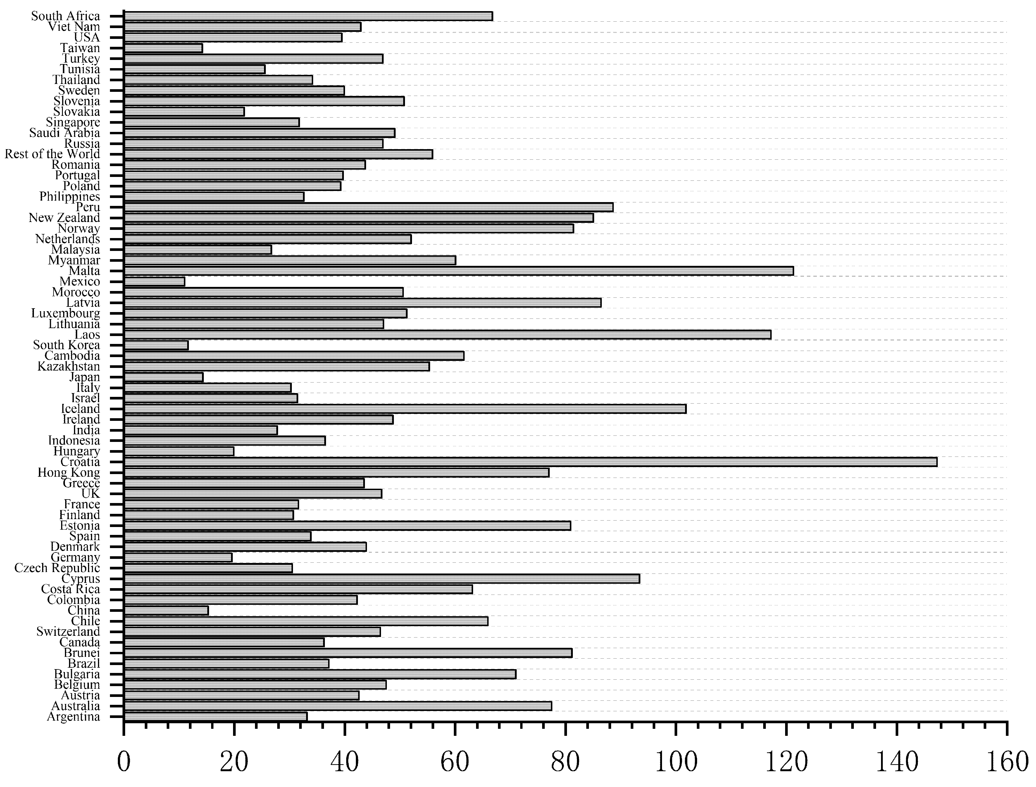
As shown in Figure 1, Iceland has the highest weighting with an average weighted degree of 99.22, followed by Cambodia with an average weighted degree of 72.83, and Saudi Arabia has the lowest weighted degree with an average of 9.37, followed by Brunei with an average weighted degree as low as 11.55, indicating that in some important forward industries, Iceland and Cambodia are more associated with other countries, while Saudi Arabia and Brunei are less associated.
As can be seen from Figure 2, Croatia maintains the highest weighted degree with an average of 147.29, followed by Malta with an average weighted degree of 121.30, and Mexico has the lowest weighted degree with an average of 11.01, followed by Taiwan, China with a low average weighted degree of 14.21, indicating that in some important backward industries, Croatia and Malta are more associated with other countries, while Mexico and Taiwan, China are less.
Overall, the average weighted value of backward industries for all countries worldwide is 50.42, which is higher than the average weighted value of forward industries, which is 37.31, indicating that most countries put most of their efforts into developing backward industries.

Node-Based Closeness Centrality

Closeness centrality is defined as a node’s proximity to other nodes in the network. The shorter the distance between a node and all other nodes, the higher its closeness centrality. First, in the hypergraph, convert it to a 5-line graph, then calculate the closeness centrality of all apices in the line graphs (the corresponding hyperedges in the hypergraph), then find all hyperedges of size k among the hyperedges to which node i belongs and sum their closeness centrality:
c _ c l o s e i k = 1 k i h E , h = k c _ c l o s e h   ( 2 < = k < = D )
The closeness centrality of each node at each order of interaction is calculated and converted into a vector, c _ c l o s e i = c _ c l o s e 2 , c _ c l o s e 3 , , c _ c l o s e D . In the higher-order interaction network of the forward or backward industrial value chain, the larger the size of the apex’s closeness centrality vector element indicates, the shorter the distance from the node to other nodes in the hypergraph, and the more the apex is in the core position in that hyperedge, indicating that the country is in the core position in the development of that industry.

Node-Based Betweenness Centrality

Betweenness centrality is defined as the frequency of nodes passing through the shortest paths among other nodes, and the higher a node’s betweenness centrality, the more frequently it becomes a “must-pass node” for the shortest paths among other nodes. The betweenness centrality of an apex in the hypergraph is still calculated by first transforming it into a line graph and then adding the betweenness centrality of the corresponding nodes in the line graph:
c _ b e t w e e n i k = 1 k i h E , h = k c _ b e t w e e n h   ( 2 < = k < = D )
The betweenness centrality of each node is calculated at each order of interaction and is used to create a vector of intermediate centrality scores, c _ b e t w e e n i = c _ b e t w e e n 2 , c _ b e t w e e n 3 , , c _ b e t w e e n D . The larger the size of the betweenness centrality vector element of the apex in the higher-order interaction network of the forward or backward industry value chain, the stronger the “bridge” role of the apex in the hypergraph, and the more mature the country’s development in the industry.

Node-Based Eigenvector Centrality

High eigenvector centrality is defined as the number of neighboring nodes that are more important than the node itself in the network. The steps for calculating the eigenvector centrality of nodes in the hypergraph are the same as in the above algorithm, except that it is first transformed into a line graph and then summed over the eigenvector centrality of the corresponding nodes in the line graph:
c _ e i g e n i k = 1 k i h E , h = k c _ e i g e n h   ( 2 < = k < = D )
The eigenvector centrality of each node is calculated at each order of interaction, yielding an eigenvector centrality vector, c _ e i g e n i = ( c _ e i g e n 2 ,   c _ e i g e n 3 , ,   c _ e i g e n D ). The size of the characteristic eigenvector centrality vector element of a node in the higher-order interaction network of the forward or backward industrial value chain shows how important the node’s neighbors are in the hypergraph, how important the country’s resources are to the development of the industry, and how competitive the country is in the development of the industry.

Node-Based Cycle Ratio

Fan, T. et al. [47] discovered that the cycle ratio can be used to determine the importance of nodes in a network. Consider the network G(V, E), where V is the set of nodes in the network, E is the set of neighboring edges between nodes, and the circle contains the shortest loop number of node i . S i represents the shortest set of circles passing through node i while S represents the shortest set of circles composed of all nodes in the network G. defined the loop structure matrix C = c i j N × N of G, where c i j is the number of loops in the set S through nodes i and j. The cycle ratio is an index used to figure out how important a node is. Here’s how it’s defined:
r i = 0 , c i i = 0 j , c i j > 0 c i j c j j , c i i > 0
when i = j , c i j is the number of circles in S that contain the node i . When i j , c i j is the number of circles in S that contain both nodes i and j. In the higher-order interaction networks of forward and backward industrial value chains, the larger the circle ratio of a node, the more important it is in the network and the more important the country has become in all industries.
The circle ratios of some countries ranked in 2000 and 2018 are shown in Table 1. China has the highest cycle ratio in the forward industrial value chain embedded network in both 2000 and 2018, 4.577 and 5.143, respectively, while the circle ratio of the backward industrial value chain embedded network is around the middle of 2.603541 and 2.362078, respectively, and the circle ratio of China in the backward industrial value chain embedded network is around the middle of the range. Russia has the highest circle ratio in the backward industrial value chain embedded network, with a value of 3.649 in 2000 and 3.332 in 2018. This shows that Russia has an important place in the network, which is related to its long-standing “processing trade” mode.

4.2.2. Hyperedges-Based Indicators Analysis

Hyperedges-Based Importance Analysis

The hypergraph is transformed into a line graph by extending the node-based cycle ratio to the higher-order network, and the importance of the hyperedge is determined by calculating the circle ratio value based on the hyperedge. The hyperedge replaces the node in the node-based circle ratio calculation method. A larger value of the circle ratio of a hyperedge in the higher-order interaction network of the forward or backward industrial value chain indicates that the hyperedge is more important in that hypergraph and that the development of that industry is more important (Table 2).
In the forward industry value chain embedded network, D21 (pharmaceuticals, pharmaceutical chemicals, and plant products) has the highest circle ratios of 31.610 and 27.775, respectively, indicating that pharmaceuticals, pharmaceutical chemicals, and plant products are more important in the forward industry. D01T02 (agriculture, hunting, and forestry) has the highest cycle ratios in the backward industry value chain embedded network, with 28.101 and 30.501, indicating that agriculture, hunting, and forestry are more important in the backward industry. D denotes the industry code according to the industry classification method of the input-output table issued by the OECD (Organization for Economic Co-operation and Development).

Hyperedges-Based Similarity Analysis

The concept of the industry similarity was introduced by Hidalgo et al. [45]. The similarity of industry i and industry j is defined as follows:
ϕ i , j = m i n P R C A x i R C A x j , P R C A x j R C A x i
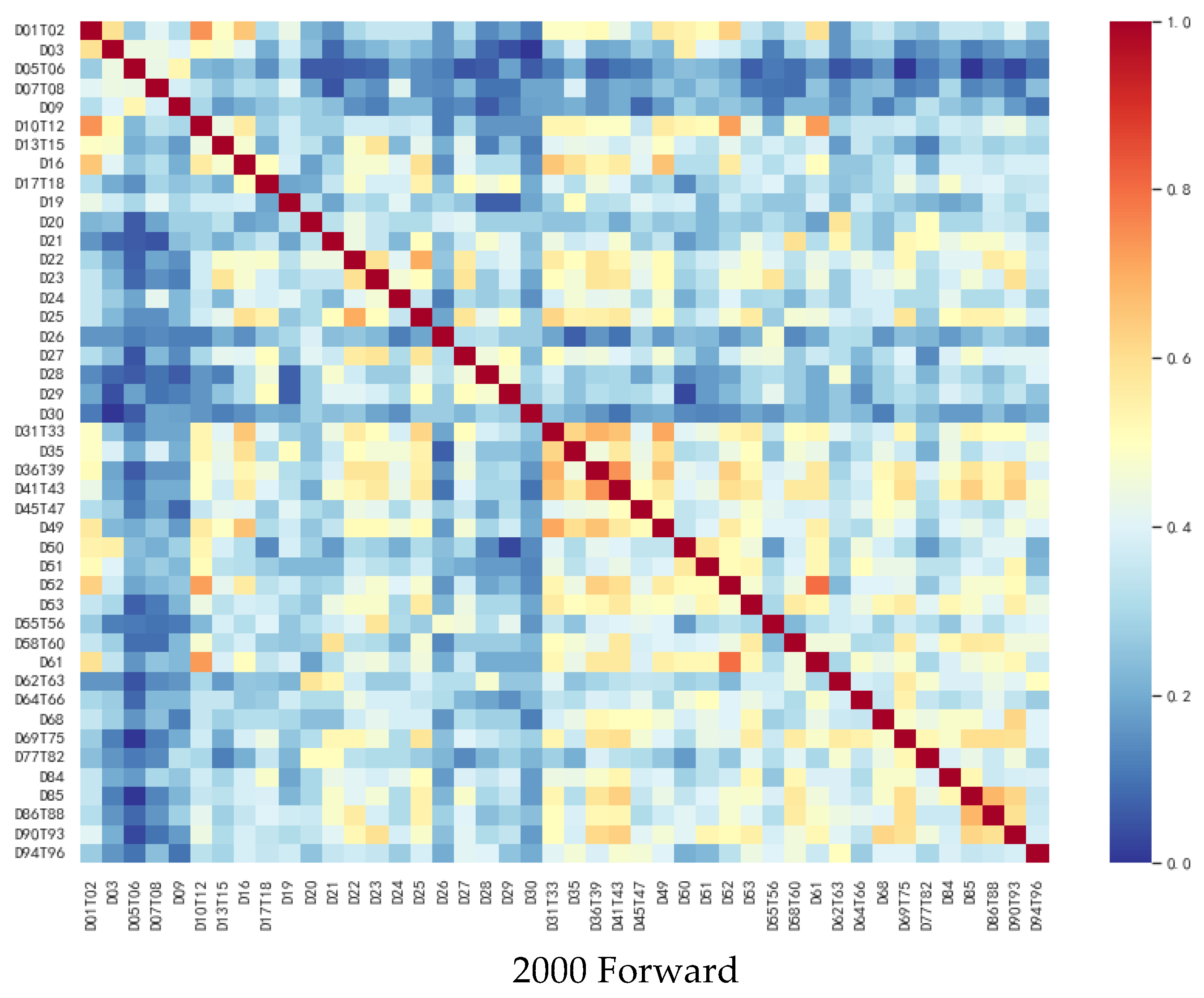
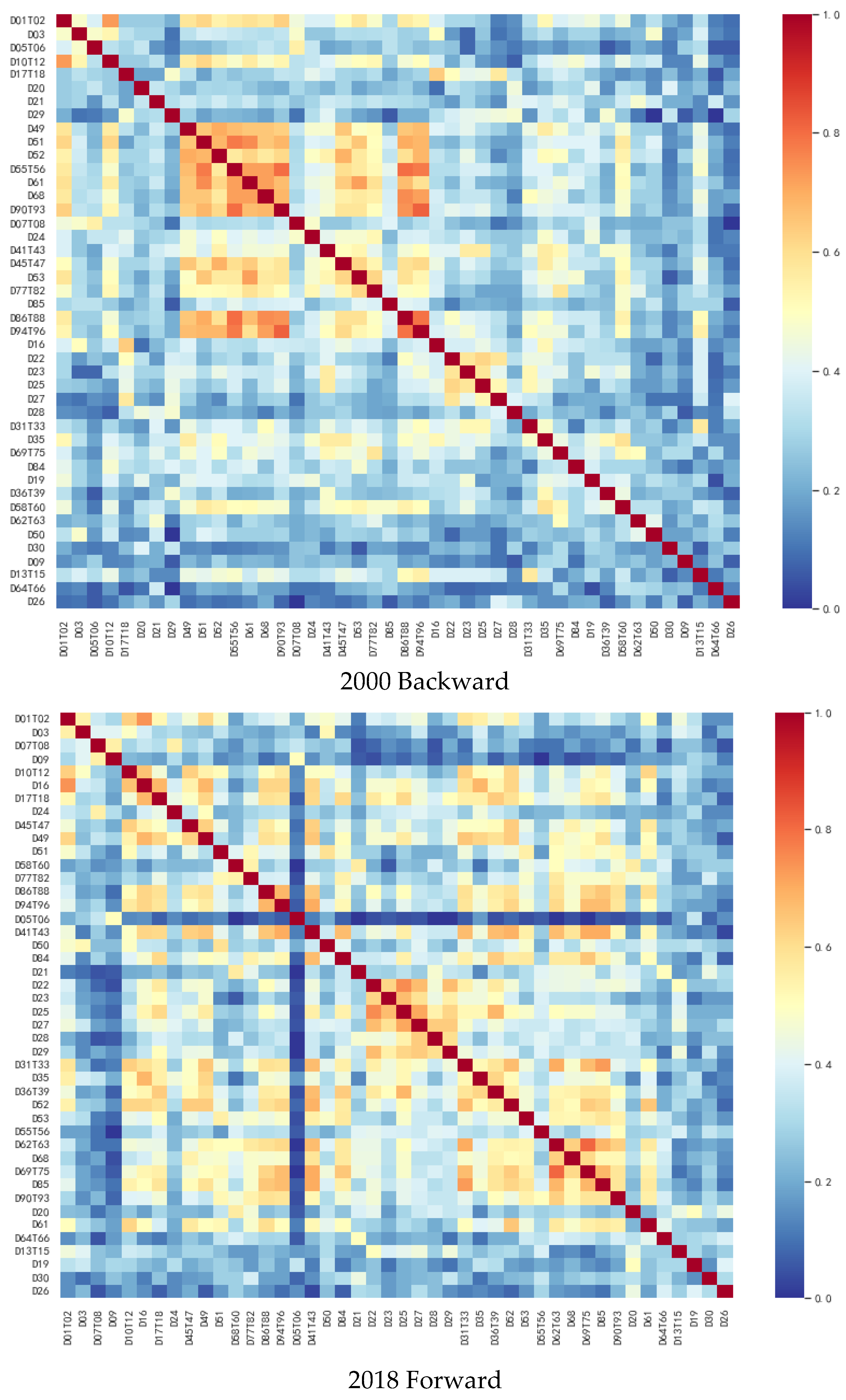
Many factors, including labor, land, capital intensity, technological maturity, and inputs and outputs in the industry value chain, lead to product correlation. Hidalgo et al. argued that if two major industries are related to each other due to similar infrastructure, physical factors, technologies, or services, they are relatively more likely to be developed by the same country, which is defined as “industry similarity” [45]. The similarity of hyperedges in the higher-order interaction network of the forward or backward industrial value chain measures which industries are concentrated in the forward or backward industrial value chains, respectively. More research can show which industries are mostly concentrated in the forward and backward industrial value chains in each country around the world.
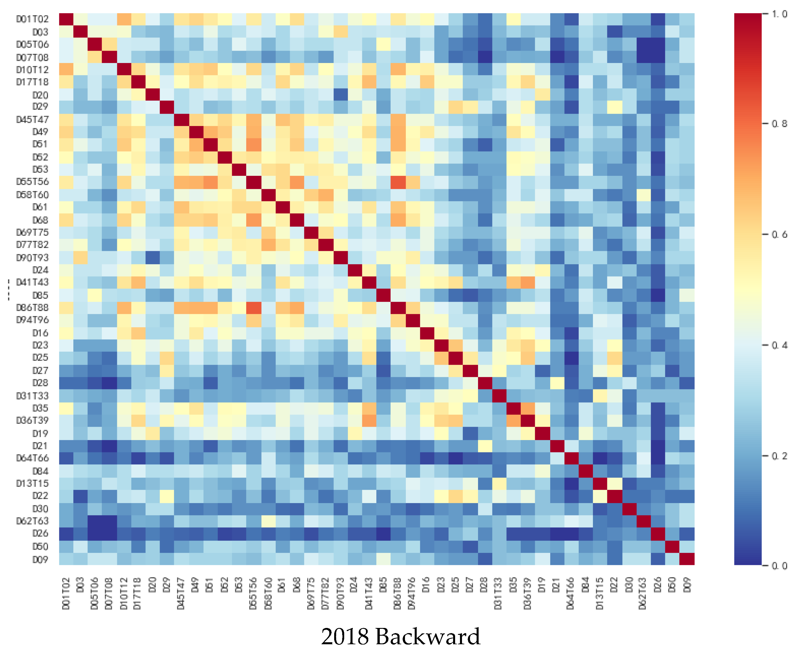
Figure 3 presents heat maps of the forward and backward industries’ similarity matrices from 2000 to 2018. The industries with higher similarity in the forward industry value chain embedded network in 2000 are primarily concentrated in the lower right side of the figure, where the similarity is higher among maintenance and installation of machinery and equipment; electricity, gas, steam, and air conditioning supply; sewage treatment; waste management and remediation; and land transportation, indicating that more countries are developing these forward-looking industries at the same time. The greater the resemblance among education, human health, social work activities, the arts, and entertainment, the more these countries are developing these industries at the same time. In the year 2000, the industries with the highest similarity in the backward industry value chain embedded network were concentrated in human health and social activities, air transportation, warehousing, and transportation support activities, accommodation and food services, telecommunications, real estate, the arts, and entertainment industries, indicating that more countries are simultaneously developing the backward industries of entertainment, services, and transportation.
In 2018, the range of industries with high similarity in the forward industry value chain embedded network tends to expand, with a focus on rubber and plastic products, other non-metallic mineral products, metal products, electrical equipment, motor vehicles, real estate activities, professional, scientific, and technological activities, education, arts, and entertainment, indicating that more countries are developing both the chemical industry and electrical equipment. Land transport and pipeline transport, air transport, warehousing and transport support activities, postal and courier activities, accommodation and food service activities, telecommunications, real estate activities, human health and social work activities are the backward industries with higher similarity in the value chain embedded network in 2018.

4.3. Networks Analysis of Global Trade Implied Carbon Emissions

The directed networks of trade-implied carbon transfer from 2000 to 2018 were constructed and analyzed by calculating relevant indicators to discover the evolutionary trend of each country’s trade-implied carbon footprint.
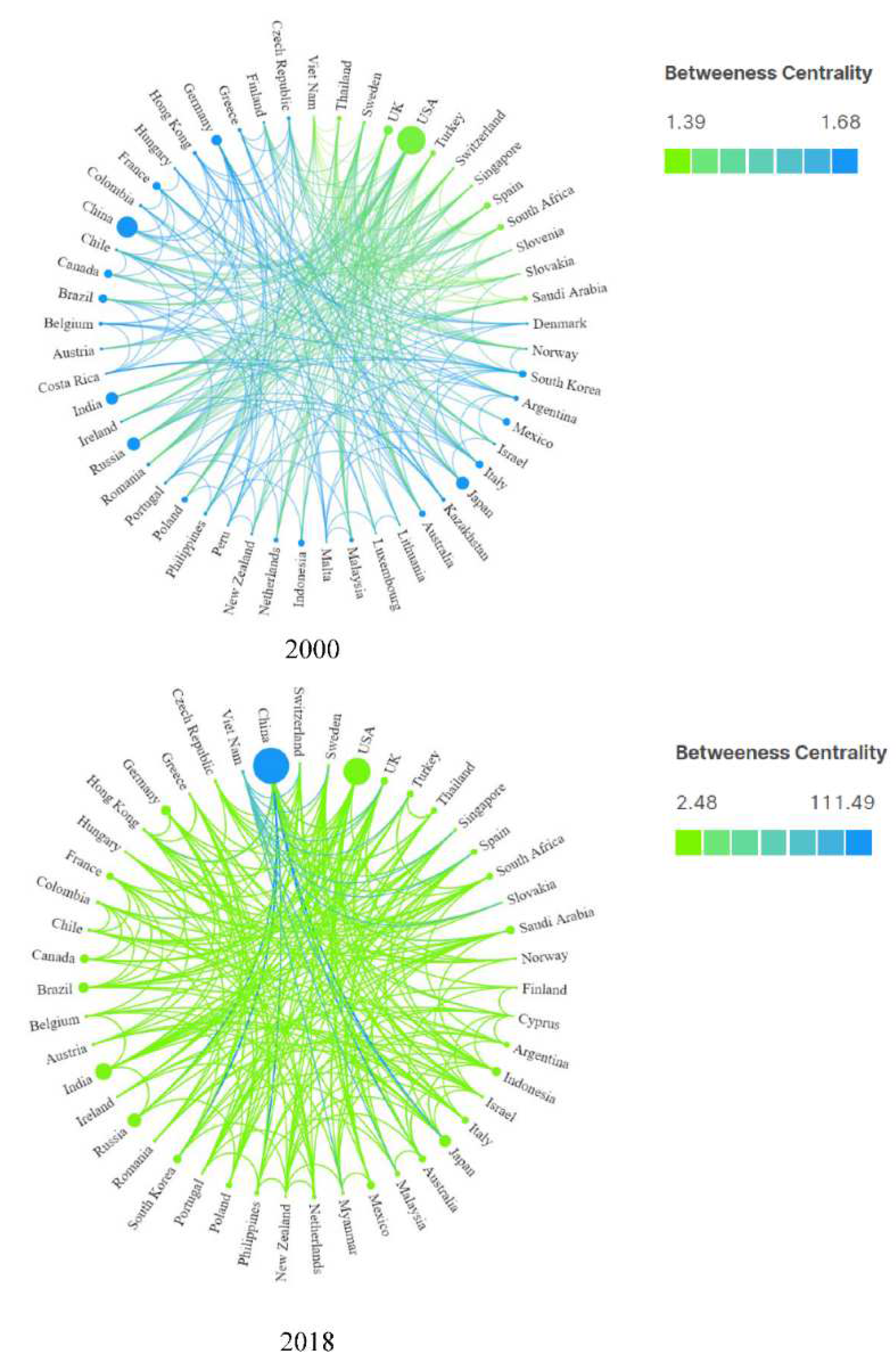
We found that the overall structural evolution of the network from 2000 to 2018 did not differ significantly, with an average network density of 1.004, an average network diameter of 2.052, an average clustering coefficient of 0.989, and an average path length of 1.006. The trade implied carbon emissions network evolved, becoming denser overall and having a smaller network diameter. As illustrated in Figure 4, the weighted degree is expressed by node size, and the color change from green to blue indicates the betweenness centrality of nodes from small to large, furthermore, the country’s position in the trade implied carbon emissions networks shifts from low to high. Most countries had a high position in the carbon emission network in 2000, and the relationships of carbon linkages among countries were generally closer, whereas in 2018, most countries’ carbon emission positions declined, and the intensity of carbon flows decreased, indicating that countries around the world have made some progress toward low-carbon sustainability. On the other hand, China’s carbon emissions are still linked to those of Russia, South Korea, the Philippines, Australia, and Japan.
Centrality is an important indicator to measure the characteristics of nodes in the network. Table 3 and Table 4 display the weighted indegree and weighted outdegree of the top ten countries from 2000 to 2018, respectively. The top ten countries fluctuate less over time, indicating that the trade-implied carbon emissions networks are stable. China’s weighted indegree and weighted outdegree in the global trade implied carbon emissions network increase over time, suggesting that China is greatly integrated into the trade implied carbon transfer networks while embedded in global industrial value chains. However, China’s weighted indegree is lower than its weighted outdegree, and China is a net carbon exporter in terms of carbon emissions, indicating that China is a “spillover” country in the trade implied carbon emissions networks. This is a global dilemma that many developing countries are currently facing. “Carbon Transfer” and “Carbon Leakage” are widening the production and consumption gaps between developed and developing countries.
The table shows the top ten countries in the weighted indegree and weighted outdegree rankings from 2000 to 2018, and their closeness centrality and betweenness centrality are both less than 1. The closeness centrality and betweenness centrality of most countries are equal to 1, and since they are positively correlated, the following filtering is done, for the carbon emissions networks, the higher the centrality indicates that the country is more important in the carbon emissions networks and occupies a certain position. For both carbon-absorbing and carbon spillover countries, they are all detrimental to national development, therefore, the lower the centrality, the more appropriate the carbon flow is. Thus, as can be seen from Table 5, of the top ten countries in terms of weighted in and weighted out in 2000, 2006, and 2012, only the USA and the UK have a centrality below 1. This means that the USA and the UK can weaken their position in the carbon emissions networks while still developing. They are also less likely to form carbon emission relationships and intensity “intermediate effects” with other countries, which is good for their environment. In 2018, the number of countries with a centrality of less than 1 went up, which shows that more and more countries are trying to develop while weakening their carbon emissions.

5. Methods, Data Source and Hypotheses

5.1. Methods

Higher-order networks are better at discovering the true topological structure of networks than traditional low-order networks, which aids in the discovery of new research conclusions. After analyzing the higher-order topology structure of global industrial value chains with different embedded methods and their evolutionary characteristics through higher-order networks, the LMDI (Logarithmic Mean Divisia Index) model is constructed based on the industrial perspective by using the LMDI decomposition method [48] to decompose the influence effect of trade-implied carbon emissions. The LMDI factor decomposition method has a high degree of rationality and scientific validity among the many index decomposition methods. Second, based on the country’s perspective, a temporal exponential random graph model is constructed, which aids in the combination of quantitative and relational perspectives. The model is fitted, and parameters are modified using maximum pseudo-likelihood estimation and Markov Monte Carlo simulation to finally obtain the dynamic influence mechanisms. It is so much better at capturing network causal relationships than traditional econometric models that enrich research conclusions. Based on a network perspective, the paper aims to analyze the influence mechanism of global industry value chain embedded on the association of trade-implied carbon emission networks from multiple dimensions.

5.2. Data Source

The relevant data in this paper are from the OECD input-output tables published from 2000 to 2018 for a total of 45 industries in 65 major countries and regions worldwide. The OECD is the Organization for Economic Co-operation and Development, with a large online statistical database, a relatively large number of members, and richer data. The country data are obtained from the satellite accounts in the EU input-output database, where the direct carbon emission factors are calculated from the emissions data in the WIOD database. Due to the incomplete data on implied emissions of global industry trade, which causes some inconvenience to the measurement, this paper aims to find the carbon emission data of global industry based on the European Union website [49], and the years of research data are all from 2000 to 2018. Partially missing data are predicted by interpolation fill and the moving average method.

5.3. Hypoyheses

5.3.1. A Hypothesis of the Factors Influencing Trade Implied Carbon Emissions Based on industry Perspective

The scale effect primarily refers to the scale of industrial output, and carbon emissions from product trade demand have been the primary source of carbon emissions in a country [50]. The structural effect refers to the effect brought about by an industrial structure, which has a significant impact on a country’s energy efficiency, and some industries have a greater impact on carbon emissions, such as textile, sewing, and leather manufacturing, the chemical industry, metal product manufacturing, and machinery manufacturing, which have seen the greatest increase in carbon emissions over time [51]. Changing the industrial structure can improve the country’s energy efficiency, providing scientific support for the implementation of carbon reduction strategies [52]. The intensity effect denotes the impact of the intensity of carbon emissions; carbon flows have a spillover effect, and it is a non-negligible factor in measuring the level of trade-implied carbon in a country or region. The scale effect has the greatest influence on trade-implied carbon emissions, and the growth of industry size is the main factor driving the increase in carbon emissions in a country. Over time, the structural effect on trade-implied carbon emissions shifts from positive to negative and then back to positive effects, while the intensity effect shifts from positive to negative and back to positive effects [53]. Some scholars have empirically discovered that the scale effect increases the carbon emission effect, and the effect of the structural effect on the implied carbon emission of trade may be promoting or inhibiting because the ways of export trade structures and export objects of different countries are different, so the structural effect does not directly reflect its constant law of action. The scale effect has the greatest impact, while the structure effect has the least [54]. The intensity effect is influenced by the heterogeneity of different industrial sectors, which has both positive and negative effects on the implied carbon emissions of trade [55].
As a result, the following hypotheses regarding the factors influencing trade-implied carbon emissions at the industry level are proposed in this paper.
H1. 
The scale effect contributes positively to the growth of trade-implied carbon emissions.
H2. 
There is a mixed effect of structural effects on trade-implied carbon emissions growth.
H3a. 
The intensity effect has a mixed effect on trade implied carbon emissions growth.

5.3.2. A Hypothesis on the Impact of Industrial Value Chains Embedded in Trade Implied Carbon Emissions Based on Industry Perspective

A country’s carbon emissions level does not necessarily represent all of the carbon dioxide emitted by it in reality and is largely due to negative externalities caused by an unbalanced pollution flow pattern in space. In the long run, the carbon flow pattern between countries forms a dynamic and complex network based on time and space, which is a directional weighted time-varying network, and at a certain time, when country A emits carbon pollutants to country B, a directed weighted edge forms from node A to node B. Because a net carbon emission effect occurs within countries, the weighting from country A to country A remains, indicating the domestic carbon emission intensity of country A. As a result, the greater the correlations between countries’ carbon emissions, the greater the mobility of carbon pollutants between countries. In the long run, the “carbon spillover” countries’ carbon pollutant emissions are relatively large and frequently emitted to other neighboring countries, causing unnecessary harm to other countries’ environmental levels while alleviating pollution problems caused by carbon emissions in their own countries. For ‘carbon receiving’ countries, which emit relatively little carbon pollution but frequently suffer from the negative externalities of other countries’ carbon pollution, although their carbon pollution is relatively small, the increasing linkage of the implied carbon emission network of global trade will undoubtedly lead to an increase in carbon pollution in their own countries for a long time, and thus these countries frequently suffer from negative externalities caused by carbon pollutants emitted by other countries. These countries have to pay a high price for environmental treatment. Many studies on the impact of industrial value chains on trade implied carbon emissions have failed to recognize this point, and the majority of them simply conclude with the positive or negative impact of industrial value chain embedded in trade implied carbon emissions using econometric models, without realizing that there is an invisible inequity between upstream and downstream industries, as well as between countries with different carbon emission attributes. Based on this “unfair” phenomenon, our study identifies the source of the problem and proposes a solution. As a result, the environmental effects of value chain embedded must be assessed by distinguishing the embedded methods of various industrial value chains and countries with varying carbon emission characteristics. The international trade dependence network tends to be stable over time [56], and the trade-implied carbon emissions depend to some extent on the trade linkage attributes, so we assume that the international trade-implied carbon emissions network still has other characteristics that change over time, including but not limited to stability.
This paper proposes the following hypothesis about the mechanism of country-level industrial value chain embedding’s influence on trade implied carbon emissions.
H3b. 
The greater the intensity of carbon emissions generated, the more global trade implied carbon emission linkages and the denser the network.
H4. 
Countries with varying carbon emission characteristics have different higher-order structural characteristics of their various industrial value chain embedded methods, as well as varying control effects on the mechanism of trade implied carbon emissions.
H5. 
The global trade implied carbon emission linkage network is characterized by spillover, stability, transferability, spontaneity, and innovation.

6. An Industry Perspective on the Factors Influencing Implied Carbon Emissions from Global Trade

6.1. LMDI Model Construction

In this paper, we use Kaya’s constant equation and the LMDI decomposition principle to build a sector-based model of the factors that affect the implied carbon emissions of trade.
C = i = 1 n C i = i = 1 n T × T i T × C i T i = i = 1 n Q × S i × R i
where C is the total trade implied carbon emissions of industrial sectors, C i is the implied carbon emissions of the industrial sector, T is the total output of industrial sectors, T i is the total output of the industrial sector, Q is the scale total, i.e., the total output of each industrial sector; S i is the industrial structure, the share of each industrial sector’s output in the total output; R i is the implied carbon emission intensity.
Because the purpose of this paper is to study the impact factors of carbon emissions at the industry level, the impact factors of implied carbon emissions are decomposed into the carbon intensity effect, industry structure effect, and output scale effect. The “output scale effect” refers to the effect of increasing output scale on carbon emissions in the industrial sector. The “industrial structure effect” is the impact of changes in industrial structure on carbon emissions in the industrial sector, while the “carbon intensity effect” is the impact of changes in carbon intensity on carbon emissions in the industrial sector. With the following equation, the total effect of implied carbon emissions from trade in the industrial sector from 2000 to 2018 is defined as Δ C , which is jointly determined by the output scale effect Δ C Q , the industrial structure effect Δ C S , and the carbon emission intensity effect Δ C R .
Δ C = C t C 0 = i = 1 n Q t S i t R i t i = 1 n Q 0 S i 0 R i 0 = Δ C Q + Δ C S + Δ C R
In order to explore the contribution of each influencing factor, the decomposition of the contribution value of each effect is as follows:
Δ C Q = i = 1 n C i t C i 0 ln C i t ln C i 0 ln Q t Q 0
Δ C S = i = 1 n C i t C i 0 ln C i t ln C i 0 ln S i t S i 0
Δ C R = i = 1 n C i t C i 0 ln C i t ln C i 0 ln R i t R i 0

6.2. Empirical Analysis of the LMDI

Overall, from Table 6, the sign of the carbon intensity effect is almost entirely negative before 2011, becomes positive from 2011 to 2016, and then reverses to be negative from 2016 to 2018. Overall, the impact of carbon intensity on carbon emissions changes from negative to positive and then back to negative, indicating that the impact of carbon intensity on carbon emissions fluctuates. The overall effect of industrial structures is positive to negative. The overall output scale effect contributes to the impact of rising carbon emissions. From 2000 to 2018, the total effect varied. The contribution rate of the carbon intensity effect is the highest from 2007 to 2008, at 264.846%; the contribution rate of industry structure is the highest from 2015 to 2016, at 5.184%; and the contribution rate of output scale is the highest from 2008 to 2009, at 20.462%.
From an industrial standpoint, in Table 7, the coke and refined petroleum industries have the greatest impact on trade implied carbon emissions, with a contribution value change of 258,683.591, followed by the mining and quarrying and energy production industries, with a contribution value change of 97,002.205. While the carbon intensity of the service sector has the greatest impact on trade implied carbon, with a contribution value change of 174.716, the output scale effect of the electricity, gas, steam, and air conditioning supply industries has the greatest impact on trade implied carbon emissions, with a contribution change of 12,701,946.12, followed by the base metal industry’s output scale effect, with a contribution change of 2,262,946.049.

7. Influence Mechanism of Global Industry Value Chain Embedded in Trade Implied Carbon Emissions

7.1. Variable Selection

The following indicator system is constructed in Table 8. The dependent variable is the probability of the existence of the implied carbon emission relationship of global trade, the degree of forward industry value chain embedding and the degree of backward industry value chain embedding, which correspond to the sender and receiver attributes, are the core explanatory variables. The sender attribute quantifies a country’s proclivity to generate more trade-implied carbon linkages with other countries, whereas the receiver attribute quantifies a country’s proclivity to receive trade-implied carbon linkages from other countries. The overall density of the trade-implied carbon emissions networks, as well as the centrality of the forward and backward industrial value chains embedded in higher-order networks, are network structure variables. The overall network density of trade implied carbon emissions, the number of relationships among trade-implied carbon emissions in the network, according to H3. In general, the denser the overall network density, the more carbon emission associations there will be. The vector centrality of the network indicates the importance of the country in the network of trade implied carbon emissions. The more important a country’s status is, the more carbon flow associations it has in the network. The k-dimensional feature vector centrality of each country in different industries from 2000 to 2018 is calculated using Equation (26), and PCA is used to reduce the multidimensional feature vector centrality to one dimension. The result of PCA reduction is incorporated into the network’s structural variables, and the reduced result indicates each country’s integrated development status in various industries. Taking into account the structure effect, scale effect, technology effect, and environmental regulation effect on trade implied carbon emissions, GDP per capita is represented as the scale effect. The economic structure determines the structure of exported products, the greater the energy consumption of exported products, the greater the trade-implied carbon emissions. The manufacturing industry plays an important role in determining a country’s productivity level; the higher a country’s share of manufacturing value added in GDP, the higher the country’s productivity level and the higher the trade implied carbon emissions from producing export products. The technology effect is expressed by the country’s R&D expenditure as a share of GDP. The higher the share, the higher the country’s technology level, which also indicates that the more resources it consumes in its technological activities, and the greater the impact on trade implied carbon emissions. According to Kheder (2008) [57], energy efficiency is a measure of the stringency of environmental regulations that can provide a more realistic reflection of the actual effect of environmental regulation policies. The time-dependent variables include “stability”, “auto”, “loss”, and “innovation”. According to H5, the trade implied carbon emission network is considered to have these time-dependent properties.

7.2. Model Construction

In general, many factors influence the formation of network relationships, including both exogenous and endogenous mechanisms that influence the evolution of network structure [58]. A series of social processes influence networks, which are activities with social properties formed by the interaction of social actors, in which the network forms certain network patterns through self-organized social processes, thus influencing other individuals in the network. The influence caused by the network’s local effects is referred to as the network’s endogenous mechanism. External factors influence the network, and this external influence is referred to as an “exogenous mechanism.” The exogenous mechanism includes the social process of the global industrial value chain embedded in the higher-order network, where the actor attributes are divided into sender attributes and receiver attributes, and the exogenous situational factors are the spatial effects of the implied carbon emissions of global trade. This paper used Temporal Exponential Random Graph Models (TERGM) to investigate the effect of global industrial value chain embedded in trade-implied carbon emissions.
The Exponential Random Graph Model (ERGM) and its extension, the Temporal Exponential Random Graph Model (TERGM), have received widespread attention and recognition as emerging network statistics methods among academics. ERGM and TERGM are methods for explaining the presence or absence of network relationships in social networks. The method overcomes the independence assumption in traditional regression methods by combining different types of micro network structures to deal with complex network dependencies and estimate their effects on network formation and evolution [5], and its greatest advantage is that it can study both endogenous and exogenous network formation mechanisms. TERGM works by fitting using maximum pseudo-likelihood estimation, simulating and parameter correcting the model through estimation, simulation, diagnosis, comparison, and improvement steps, and finally obtaining empirical estimation results that converge to stability. Its main benefit is that it can be used to study dynamic observation networks and takes into account network data that change over time [5].
The measured network data from 2000 to 2018 is used to explore endogenous mechanisms such as higher-order network structure dependence and time dependence of forward and backward industrial value chain embedding under the influence of exogenous mechanisms, and to quantitatively analyze the probability of relationships. The following is how the time-exponential random graph model (TERGM) is built:
P 1 N t θ t , N t 1 = 1 / c exp θ 0   edges   + θ 1   stability + θ 2   auto + θ 3   loss + θ 4   innovation + θ 5   geo + θ 6   GVC _ IV + θ r 1 ln G D P + θ r 2 q _ eig + θ r 3 structure + θ r 4 tec + θ r 5 energy + θ s 1 ln G D P + θ s 2 q _ eig + θ s 3 structure + θ s 4 tec + θ s 5 energy
P 2 N t θ t , N t 1 = 1 / c exp β 0   edges   + β 1   stability + β 2   auto + β 3   loss + β 4   innovation + β 5 geo + β 6 GVC _ FV + β r 1 ln G D P + β r 2 h _ eig + β r 3 structure + β r 4 tec + β r 5 energy + β s 1 ln G D P + β s 2 h _ eig + β s 3 structure + β s 4 tec + β s 5 energy
where Equation (40) represents the forward industry value chain embedding effect on trade-implied carbon emissions, and Equation (41) represents the backward industry value chain embedding effect on trade implied carbon emissions. N t , N t 1 denote the trade implied carbon emissions network at time t and t-1, respectively, and correspond to the unknown parameters, the subscript of r represents the receiver, s represents the sender, and 1 / c is the normalization constant to ensure the network is not distorted. The chances are kept between 0 and 1. The edges in the network of traded implied carbon emissions show the side variables, which are the same as the intercept terms in a traditional regression model.

7.3. Analysis of Empirical Results

7.3.1. Empirical Analysis of the TERGM

According to Table 9, the network edges are significant at the 1% level with positive coefficients, indicating that the more carbon emissions relationships each country has, the denser the trade implied carbon emissions networks are. Among the receiver attributes, the coefficient of the core explanatory variable “GVC_IV” is significantly negative at the 1% level, indicating that the deeper the “ carbon receiving country” is embedded in the forward industrial value chain, the fewer trade implied carbon emissions associations it has with other countries; the reduced dimensional eigenvector centrality “q_eig” is significantly negative at the 1% level, which means that the deeper the “ carbon receiving country” is embedded in the forward industrial value chain, the fewer trade implied carbon emissions associations it has with other countries, the more important the carbon ‘receiving country’ is embedded in the forward industry value chain, the more trade implied carbon emissions linkages it generates with other countries. The coefficient of the control variable “lnGDP” is significantly positive at the 1% level, indicating that the economy of the “carbon receiving countries” is significantly positive at the 1% level; The more developed the economy of the “carbon receiving country” is, the more it is associated with the trade-implied carbon emissions generated by other countries; the coefficient of the control variable “tec” is significantly positive at the 1% level, suggesting that the greater the R&D expenditure of the “carbon receiving country” is, the more it is associated with the trade-implied carbon emissions generated by other countries. The coefficient of the control variable “energy” is significantly negative at the 1% level, indicating that the stronger the environmental regulation of the “carbon receiving country”, the less it is associated with the trade-implied carbon emissions generated by other countries. While in sender attributes, the results show some variations. The “q_eig” of the higher-order structural variable forward industry value chain embedding is significantly negative at the 1% level, indicating that the more important the forward industry value chain embedded status of the “carbon spillover country” is, the less trade implied carbon emission association it has with other countries. The coefficient of the control variable “lnGDP” is significantly negative at the 1% level, indicating that the more developed the economy of the carbon emission “carbon spillover country” is, the less the trade implied carbon emissions are associated with other countries; the coefficient of the control variable “structure” is significantly positive at the 1% level, indicating that the coefficient of the control variable “structure” is positive at the 1% level, indicating that the more manufacturing value added in the “carbon spillover country”, the more the trade implied carbon emissions are associated with other countries. The network covariate “geo” is significantly positive at the 1% level, indicating that geographically adjacent countries have relatively more implied carbon emissions linkages.
Models 2–5 include the time-dependent variables: stability, transferability, dischargeability, and updatability. In Model 2, the coefficient of the time-dependent variable “stability” is significantly positive at the 1% level, indicating that the existing trade implied carbon emissions linkages have a tendency to remain stable over time, and in Model 3, the time-dependent variable “auto” is significantly positive at the 1% level, suggesting that there is a tendency for previous national carbon emission network associations to shift over time to the current network. In model 4, the coefficient of the time-dependent variable “loss” is significantly negative at the 1% level, indicating that the carbon emission associations generated by some countries before, tend to be eliminated over time, and the more elimination, the fewer carbon emission associations. In model 5, the coefficient of the time-dependent variable “innovation” is significantly negative at the 1% level. This means that there is a tendency for countries that haven’t formed carbon emission associations before to do so over time.
From Table 10, the baseline model 1 shows that the structure-dependent variable “edges” is significant at the 1% level with a positive coefficient, indicating that the more carbon emission relationships among countries, the denser the trade implied carbon emission network; in the receiver attribute, the core explanatory variable backward industry value chain embedded degree “GVC_FV” has a coefficient at the 1% level, indicating the deeper the “carbon receiver country” is embedded in the backward industry value chain, the less trade implied carbon emission associations it has with other countries; The coefficient of the reduced dimensional eigenvector centrality “h_eig” is significantly negative at the 1% level, indicating that in the receiver attribute, the more important the embedded status of the carbon emission “receiver country” in the backward industry value chain, the less trade implied carbon emission association it has with other countries. The coefficient of the control variable “lnGDP” is significantly positive at the 1% level, indicating that the more developed the economy of the carbon emission “receiver country” is, the more trade implied carbon emission associations it has with other countries. The coefficient “tec” is significantly positive at the 1% level, indicating that in the receiver attribute, the more R&D expenditure and the higher the level of scientific research, the more it is associated with the trade implicit carbon emissions of other countries. The core explanatory variable “GVC_FV” has a significant positive coefficient at the 1% level, indicating that the deeper the carbon “spillover country” is embedded in the industrial value chain, the more the implied carbon emission linkage with other countries. The coefficient of the control variable “lnGDP” is significantly negative at the 1% level, indicating that the more developed the economy of the carbon “spillover country” is, the less linkage of trade implied carbon emissions with other countries; the coefficient of the control variable “structure” is significantly positive at the 1% level, indicating that the more manufacturing value is added in the “spillover country”, the more it is associated with trade implied carbon emissions from other countries; the coefficient of the control variable “energy” is significantly positive at the 1% level, indicating that the stronger the environmental regulation in the “spillover country”, the more it is associated with trade implied carbon emissions from other countries. The network covariate geographic proximity “geo” is significantly positive at the 1% level, indicating that geographically neighboring countries have relatively more trade-implied carbon emissions linkages.
Models 2–5 include the time-dependent variables stability, transferability, dischargeability, and updatability, and their findings are consistent with the table results.

7.3.2. Multicollinearity Test

A multicollinearity test was performed, and the test results revealed that the average VIF value of each variable in the model of the effect of forward industry value chain embedded in trade implied carbon emissions is 1.22, and the average VIF value of each variable in the model of the effect of backward industry value chain embedded in trade implied carbon emissions is 1.15, both of which are significantly less than 10, indicating that there is no multicollinearity in the model.

7.3.3. Robustness Test

This paper performs robustness tests in two ways to judge the robustness of the TERGM fitting results.

Extrapolation from an Out-of-Sample

Accordingly, the dynamic network data is divided into training and test data, and 10,000 simulation networks are generated for out-of-sample extrapolation. The model is robust overall if the out-of-sample extrapolation results are similar to the original model results. Otherwise, the model is not robust. The impact of forward and backward industrial value chain embedded in trade implied carbon emissions is modeled by using data from 2000 to 2017 for the training set and data from 2018 for the test set. Model 1 in Table 11 shows the results of forward out-of-sample extrapolation, which are consistent with Model 1 in Table 9, and Model 2 in Table 11 shows the results of backward out-of-sample extrapolation, which are consistent with Model 1 in Table 10, which shows that the models are robust.

Great Likelihood Estimation Using Markov Monte Carlo

The forward and backward impact models’ estimation methods are replaced with Markov Monte Carlo maximum likelihood estimation [59], the empirical results of TERGM are shown in Table 12, where the results of Model 1 in Table 12 are consistent with the results of Model 1 in Table 9, and the results of Model 2 in Table 12 are consistent with the results of Model 1 in Table 10, indicating that after replacing the estimation method, the models are still robust.

8. Discussion

The embedded relationships and carbon emission relationships among countries and industries are becoming increasingly complex as the global industrial value chain division of labor deepens, exhibiting a more complex network characteristic. The majority of current literature discusses the influence mechanism based on a quantitative relationship between global industrial value chain embedded indicators and trade implied carbon from a structural perspective [60,61], and lacks a complex unstructured perspective to analyze the influence mechanism of value chain embedded in trade implied carbon emission linkage among countries and industries under higher-order interaction. Only a small portion of the literature has used social network analysis to examine low-order network characteristics [62,63]. Higher-order networks are more complex than traditional low-order networks in terms of topological complementary structure and evolutionary laws because they are more realistic and complex as they approach real-world network complexity [64]. In order to make the research conclusions more objective, the higher-order networks are interestingly integrated with environmental, economic, and social issues under one framework for the first time. Unlike previous studies, this paper discovers the “importance degree” of different countries in each forward and backward industry, respectively by constructing the higher-order networks of forward and backward global industrial value chains embedding and by calculating the characteristic indicator vectors of vertices. Which forward and backward industries have been mainly developed in each country from 2000 to 2018, and what is the evolution trend of their development process, and it is meaningful to grasp the development process of each country in each industry for the conclusion of national import and export trade and cooperation. This paper extends the circle ratio calculation method [47], based on hyperedge and uses it to calculate the circle ratio of hyperedge in higher-order networks, which helps to discover the importance of hyperedge in higher-order networks. The hyperedge represents a certain industry developed by different countries together, and the more important the hyperedge is, the more important the industry is in the higher-order networks. Measuring important industries is important for the development of national industrial structure, which has a role in not only economic development but also in the adjustment of environmental governance policies. Calculating the hyperedge similarity can discover the degree of similarity of industries and provide a reference for industrial integration and further upgrading of industries. By calculating the comparative weighting degree, it is found that the weighting degree of backward industries is greater than that of forward industries. That is, most countries mainly develop backward industries relative to forward industries.
By constructing the trade implied carbon emission network and calculating the characteristics of relevant indicators, it is found that China is greatly integrated into the trade implied carbon transfer network while being embedded in the global industrial value chain, which is an international problem common to many developing countries nowadays, and although it is in a central position in the trade implied carbon emission network, it is more as a “producer. This is an international problem common to many developing countries, and although they are at the center of the network, they are more as “producers” than “consumers.” “Carbon transfer” and “carbon leakage” are gradually widening the gap between developed and developing countries on the production and consumption sides.
GVC embedding can be divided into forward embedding and backward embedding based on the different methods; these different embedded methods reflect the different forms of countries’ participation in the international division of labor; only a few studies have considered this distinction [65]. When selecting variables, some studies only considered a single embedded mode, resulting in a bias in the environmental effects of GVC embedding [66,67]. Most existing studies are based on a single country’s domestic industry [68,69], and there is a dearth of studies based on multiple perspectives, such as individual countries in a global context. In this paper, we combine the two and look at the factors that influence industrial carbon emissions and national trade-implied carbon emissions from the standpoints of industry and country, respectively. For the aspect of industry, according to the LMDI model, the influence factors of industrial trade carbon emissions are decomposed into carbon intensity effect, industrial structure effect, and output scale effect, with the carbon intensity effect showing a negative to positive and then negative trend, while the industrial structure effect shows an overall positive to negative trend. The overall output scale effect contributes to the impact of carbon emission growth. For the aspect of country, In terms of methodology, unlike previous studies, this paper constructs a time exponential random graph model as a network causal model, and because time-varying network data is equivalent to the integration of structured and unstructured data, the trade implied carbon emissions of the same country at different times can be regarded as panel data in structured data, while the trade implied carbon flows of the country and other covariates can be regarded as panel data in unstructured data. Furthermore, when variables are included, this paper considers the distinction between “receiver attribute” and “sender attribute,” and by distinguishing different carbon emission attributes, the conclusions obtained differ, allowing the proposed countermeasures to be more targeted. This is something that previous empirical studies have not done. This paper empirically shows that the role of forward and backward global industrial value chains embedded in trade implied carbon emissions differs for countries with different carbon flow attributes. The deeper the embedding in the forward industrial value chain of “carbon absorbing” and “carbon spillover” countries, the lower the trade-implied carbon emissions linkages with other countries. The deeper the embedding in the backward industrial value chain for “carbon absorbing” countries, the less the implicit carbon emissions linkages among the “carbon absorbing” countries and other countries; whereas for “carbon spillover” countries, the deeper the embedding in the backward industrial value chain, the less the implicit carbon emissions linkages between the “carbon absorbing” countries and other countries. The deeper the embedding of the backward industrial value chain in “carbon spillover” countries, the stronger the trade-implied carbon emissions linkages among “carbon spillover” countries and other countries. The effective paths of trade-implied carbon emissions reduction differ for countries with different carbon flow attributes. Expanding their embedding depth in the value chains of forward and backward industries, increasing the intensity of environmental regulations, and improving their embedding position in the value chains of backward industries can effectively reduce trade-implicit carbon emission linkages for “carbon absorbing” countries, while expanding their embedded depth in the value chains of forward and backward industries can effectively reduce trade-implicit carbon emission linkages for “carbon spillover” countries. For “carbon spillover” countries, increasing the depth of embedding in the forward industry’s value chain, decreasing the depth of embedding in the backward industry’s value chain, and increasing the embedded position in the backward industry’s value chain can effectively reduce the trade-implicit carbon emission linkage.

9. Conclusions and Implications

9.1. Conclusions

This paper establishes a country-based higher-order network of industrial value chain embedding and a directed network of trade implied carbon, conducts a macro-topology analysis of global industrial value chain embedding at the overall level, uses the LMDI model to analyze the factors influencing the implicit carbon emissions of trade, and uses a time exponential random graph model to test the endogenous influence mechanism affecting the correlation network of global trade implied carbon emissions. All the hypotheses are confirmed. The following conclusions are obtained:
First, there are more countries with global backward industry linkages compared to those with forward industry linkages, which is in line with the findings of Morris, M. et al. [70]. The average weighted value of backward industries in each country in the world is 50.42, which is higher than the average weighted value of forward industries of 37.31, indicating that most countries mainly focus on the development of backward industries. Backward value chain embedding is mainly in the form of processing, assembly, and other forms of participation in the global value chain division of labor. In this embedded mode for intermediate product imports, the division of labor status is low. In order to coordinate the industrial structure and avoid the impact of some industries on the country’s embedded value chain status, some countries have begun to attach importance to the balanced development of forward and backward industries. According to this conclusion, this paper believes that it may also be because the productivity level of most countries is not high enough, resulting in these countries being unable to produce backward industries for a long time. If it is based on this reason, environmental pollution causes such as carbon emissions should be given more attention.
Second, according to the Global Industry Classification Standard (GICS) industry classification criteria, we find that industries with a deeper embedding in the global forward value chain are primarily concentrated in basic materials and public utilities, whereas industries with a deeper embedding in the global backward value chain are primarily concentrated in consumer non-essential goods and real estate. The forward industry value chain embedding is mainly concentrated in machinery and equipment maintenance and installation; electricity, gas, steam, and air conditioning supply, sewage treatment, waste management, and restoration; land transportation and pipeline transportation; rubber and plastic products; other non-metallic mineral products, metal products, electrical equipment, motor vehicles, etc.; while the backward industry value chain embedding is mainly concentrated in real estate activities, professional scientific and technical activities, education, the arts, and entertainment; air transportation, warehousing, and transportation support activities; transportation; food service activities, etc. The literature [45] also studied the similarity and spatial spillover of industries with a detailed industry classification, on the basis of which this paper also delineates forward and backward industries in detail, and then investigates the similarity of all subdivided industries within them.
Third, “carbon transfer” and “carbon leakage” gradually widen the gap between developed and developing countries on the production and consumption sides, which is consistent with the findings of Ji, C.Y. and Yang, H.Q. [71], Zhou, B. et al. [72]. Although China’s weighted inward centrality is lower than its weighted outward centrality, it is a net carbon exporter in terms of carbon emissions and carbon relations, which means that China tends to be a “spillover” country in the global trade implied carbon network. This means that China tends to be a “spillover” country in the global trade implied carbon network, which is an international problem common to many developing countries, and is more of a “producer” than a “consumer,” although it is at the core of the trade implied carbon network. “Carbon transfer” and “carbon leakage” are gradually widening the gap between developed and developing countries on the production and consumption sides.
Fourth, overall, the impact of carbon intensity on carbon emissions changes from negative to positive and then back to negative, the overall effect of industrial structure is positive to negative, and the overall output scale effect contributes to the impact of rising carbon emissions. These conclusions are in line with the findings of Zhang, W. et al. [73], and Wang, B.Q. et al. [54]. The coke and refined petroleum industries have the greatest impact on trade implied carbon emissions, followed by the mining and quarrying and energy production industries, while the carbon intensity of the service sector has the greatest impact on trade implied carbon emissions. The output scale effect of the electricity, gas, steam, and air conditioning supply industry has the greatest impact on trade implied carbon emissions, followed by the base metal industry’s output scale effect.
Fifth, not all countries have embedded value chains whose affects the mechanism of trade implied carbon emissions in the same way. For countries with different carbon flow attributes, their forward and backward global industrial value chain embedded has different effects on trade-implied carbon emissions. In the case of “carbon-absorbing” and “carbon spillover” countries, the deeper the embedding in the forward industrial value chain, the lower the trade-implicit carbon emission linkage between the country and other countries. The reason is that forward value chain embedded is mainly in the form of intermediate products. It is mainly in the form of exports of intermediate products, and the status and technology content of the embedded value chain are higher. More participation in this form of global value chain division of labor is beneficial to the reduction of trade-implied carbon emissions. In backward industrial development, for the “carbon-absorbing” countries, the deeper the embedding in the backward industrial value chain, the lower the implicit carbon emission linkage between the “carbon-absorbing” countries and other countries; while for the “carbon spillover” countries, the deeper the embedding in the backward industrial value chain, the lower the implicit carbon emission linkage between the “carbon-absorbing” countries and other countries. For “carbon spillover” countries, the deeper the embedding of backward industrial value chains, the more trade-implicit carbon emission linkages there are between “carbon spillover” countries and other countries. The backward industry has more processing and production links compared with the forward industry, so it is generally believed that the backward industry is more likely to cause carbon emissions. For “carbon absorbing” countries, their carbon emissions are relatively small due to their industrial structure, and they are more passive recipients of carbon pollutants from other countries. Therefore, if these countries improve their productivity, vigorously develop the degree of embedding of backward industries, improve their core competitiveness, and improve the international status of backward industries, this is likely to create obstacles for those countries that often emit carbon dioxide, while for “carbon spillover” countries, the more vigorously they develop backward industries, the more production links they export, and the more carbon emissions they have to their own countries or even other countries. For countries with “carbon spillover”, the more they develop backward industries, the more they export production, and the more carbon emissions they imply for their own country or even other countries.
Sixth, for countries with different attributes of carbon flows, the effective paths of trade-implied carbon reduction are different. For “carbon-absorbing” countries, in terms of “objective factors,” increasing the intensity of environmental regulations can weaken the negative externalities brought by other countries, and in terms of “subjective factors,” increasing the depth of embedding in the value chains of forward and backward industries and improving the international division of labor in backward industries can effectively reduce the trade-implied carbon emissions. In terms of “subjective factors,” expanding the depth of embedding in the value chains of forward and backward industries and improving the international division of labor in backward industries can effectively reduce the trade-implicit carbon emission linkage and thus reduce the trade-implicit carbon intensity. As for “carbon spillover” countries, they should try their best to balance the development of forward and backward industries and avoid bringing negative external effects of carbon emissions to other countries while ensuring a stable and forward economic level. The “objective factors” are less restrictive, so the control of “subjective factors” should be increased, the depth of embedding in the value chain of the forward industry should be expanded, the depth of embedding in the value chain of the backward industry should be reduced, and the position of embedding in the value chain of the backward industry should be increased. The trade-implied carbon emission linkage can be effectively reduced, thus reducing the trade-implied carbon intensity.

9.2. Implications

Based on the above findings, the following countermeasures are proposed:
First, the linkages of global carbon transfer should be fully considered when implementing the implicit carbon reduction in global trade. This requires the implementation of environmental management measures not only to limit carbon emissions, but also to consider the linkage and flow of carbon emissions under the variable input-output relationship; to form a “quantity-linkage” dual control system of emission reduction, and to actively establish a transnational collaborative emission reduction mechanism.
Second, in the definition of international emission reduction, the balance between the consumption and production sides should be fully implemented to reduce the non-homogeneity of the two. Developed countries can give technical support to developing countries in carbon emission reduction, balance carbon emissions and carbon spillover while maximizing embedded in the global industrial value chain, narrow the gap between the production and consumption sides of carbon emissions in developed and developing countries as much as possible, and avoid “carbon leakage” and “carbon transfer”. Thirdly, because of the different carbon emission attributes of developed and developing countries, it is important to avoid the problem of carbon leakage and transfer.
Third, for countries with different carbon emission profiles, carbon emission reduction by trade should be carried out in a targeted manner. When formulating carbon emission reduction regulations and carbon emission reduction targets, the spatial carbon flow direction of the country should be considered, as well as the differences in industrial structure, economic level, technological level, and environmental regulation level of each country, so that carbon emission reduction plans can be reasonably formulated according to local conditions.
Fourth, to encourage the use of natural gas and other relatively clean energy, it is necessary to reduce the proportion of fossil fuels and coal in energy consumption; develop and research new energy sources, such as solar energy, wind energy, and water energy; strengthen policy support to promote energy conservation and emission reduction; increase financial investment in the research and development of low-carbon technologies and the policy support of low-carbon technology research and development, application, and popularization; support the R&D, application, and popularization of low-carbon technologies; give tax incentives to innovative enterprises, and accelerate energy conservation and emission reduction.
Fifth, in paying attention to the environmental effects of embedding in the global industrial value chain, each country should not only focus on the adjustment of the embedded mode, but also on the embedded relationship, which not only refers to the breadth and depth of the industrial relationship but also includes the control of the embedded relationship. That is, if a country’s position in the embedded network rises, the country will occupy a dominant position in the industrial embedded relationship and have certain core competitiveness. In other words, if a country’s position in the embedded network rises and the country occupies a dominant position in the industrial embedded relationship and has certain core competitiveness, the country will be able to give priority to its initiative to resist the negative environmental externalities brought about by the embedding of the value chain through industrial transformation, industrial integration, industrial upgrading, and other means. Therefore, China should actively establish industrial-embedded relationships with other countries, continuously optimize the quality of the relationships, and enhance their positive externalities.

Author Contributions

Conceptualization, C.L. and X.Z.; methodology, X.Z.; software, X.Z.; validation, C.L. and X.Z.; formal analysis, X.Z.; investigation, C.L.; resources, C.L.; data curation, X.Z.; writing—original draft preparation, X.Z.; writing—review and editing, C.L.; visualization, X.Z.; supervision, C.L.; project administration, C.L.; funding acquisition, C.L. C.L. and X.Z. are the co-first authors, X.Z. is the corresponding author. All authors contributed equally to this work. All authors have read and agreed to the published version of the manuscript.

Funding

This research was supported by the National Social Science Funding of China, grant number (18BJY081).

Institutional Review Board Statement

Not applicable.

Informed Consent Statement

Not applicable.

Data Availability Statement

Relevant data about the value chain is from OECD Data Platform (https://data.oecd.org/, accessed on 8 August 2022). The emissions data is from WIOD Platform (https://www.rug.nl/ggdc/valuechain/wiod, accessed on 5 September 2022). The carbon emission data of global industry is from the European Union website (https://ec.europa.eu/jrc/en/research-topic/economic-environmental-and-social-effects-of-globalisation, accessed on 17 September 2022).

Acknowledgments

Thanks to the editors and reviewers for their comments; our article has been greatly improved. Moreover, we would like to thank Hebei GEO University (KJCXTD-2022-02) for providing us with the necessary financial support.

Conflicts of Interest

The authors declare no conflict of interest.

References

  1. Porter’s, V.C.M. What Is Value Chain; The Free Press: New York, NY, USA, 1985; pp. 1–13. [Google Scholar]
  2. Du, Y.S.; Peng, D.D. The servitization of manufacturing and the upgrading of global value-added trade network status-based on the world input-output tables from 2000–2014. Financ. Trade Econ. 2018, 39, 102–117. [Google Scholar]
  3. Grossman, G.M.; Rossi-Hansberg, E. Trading tasks: A simple theory of offshoring. Am. Econ. Rev. 2008, 98, 1978–1997. [Google Scholar]
  4. Hummels, D.; Ishii, J.; Yi, K.M. The Nature and Growth of Vertical Specialization in World Trade. J. Int. Econ. 2001, 54, 75–96. [Google Scholar]
  5. Zeng, Z.; Zhang, L.L. Defining the distribution of trade benefits between China and the United States under the global production network system—A study on the value added of China’s manufacturing trade. World Econ. Stud. 2008, 1, 36–43. [Google Scholar]
  6. Johnson, R.C.; Noguera, G. Accounting for Intermediates: Production Sharing and Trade in Value Added. J. Int. Econ. 2012, 86, 224–236. [Google Scholar] [CrossRef] [Green Version]
  7. Koopman, R.; Powers, W.; Wang, Z.; Wei, S.J. Give Credit Where Credit is Due: Tracing Value Added in Global Production Chains; NBER Working Paper Series; National Bureau of Economic Research: Cambridge, MA, USA, 2010. [Google Scholar] [CrossRef]
  8. Wang, Z.; Wei, S.J.; Zhu, K. Quantifying International Production Sharing at the Bilateral and Sector Levels; NBER Working Paper Series; National Bureau of Economic Research: Cambridge, MA, USA, 2013. [Google Scholar] [CrossRef]
  9. Koopman, R.; Wang, Z.; Wei, S.J. Tracing Value—Added and Double Counting in Gross Exports. Am. Econ. Rev. 2014, 104, 459–494. [Google Scholar]
  10. Wang, Z.; Wei, S.J.; YU, X.; Zhu, K. Measures of participation in global value chains and global business cycles. Natl. Bur. Econ. Res. 2017. [Google Scholar] [CrossRef]
  11. Matthew, C.; Mahutga, M.C. When do value chains go global? A theory of the spatialization of global value chains. Glob. Netw. 2012, 12, 1–21. [Google Scholar] [CrossRef]
  12. Hipp, A.; Binz, C. Firm Survival in Complex Value Chains and Global Innovation Systems: Evidence from Solar Photovoltaics. Res. Policy 2019, 49, 103876. [Google Scholar] [CrossRef]
  13. Knez, K.; Jaklič, A.; Stare, M. An extended approach to value chain analysis. J. Econ. Struct. 2021, 10, 1–37. [Google Scholar] [CrossRef] [PubMed]
  14. Wyckoff, A.W.; Roop, J.M. The Embodiment Carbon in Imports of Manufactured Products: Implements for International Agreements on Greenhouse Gas Emissions. Energy Policy 1994, 22, 187–194. [Google Scholar]
  15. Mäenpää, I.; Siikavirta, H. Greenhouse Gases Embodied in the International Trade and Final Consumption of Finland: An Input-Output Analysis. Energy Policy 2007, 35, 128–143. [Google Scholar]
  16. Wiedmann, T.; Minx, J.; Barrett, J.; Wackernagel, M. Allocating Ecological Footprints to Final Consumption Categories with Input-Output Analysis. Energy Policy 2008, 25, 245–258. [Google Scholar]
  17. Liu, X.; Ishikawa, M.; Wang, C.; Dong, Y.; Liu, W. Analyses of CO2 Emissions Embodied in Japan-China Trade. Energy Policy 2010, 38, 1510–1518. [Google Scholar]
  18. Du, H.; Guo, J.; Mao, G.; Smith, A.M.; Wang, X.; Wang, Y. CO2 Emissions Embodied in China-US Trade: Input-Output Analysis Based on Energy/Dollar Ratio. Energy Policy 2011, 39, 5980–5987. [Google Scholar]
  19. Li, H.M.; Qi, Y. Carbon Embodied in International Trade of China and its Emission Responsibility. Chin. J. Popul. Resour. Environ. 2010, 8, 24–31. [Google Scholar]
  20. Lin, B.Q.; Sun, C.W. Evaluating Carbon Dioxide Emissions in International Trade of China. Energy Policy 2010, 38, 613–621. [Google Scholar]
  21. Shui, B.; Harriss, R.C. The role of CO2 embodiment in US–China trade. Energy Policy 2006, 34, 4063–4068. [Google Scholar]
  22. Wang, Y.Y.; Yan, Y.Y.; Li, L. Implicit carbon emission flows in the international trade of computer products. China Popul.-Resour. Environ. 2015, 25, 37–40. [Google Scholar]
  23. GrossmanGM, K. Environmental Impacts of the North American Free Trade Agreement; NBER Working Paper Series; National Bureau of Economic Research: Cambridge, MA, USA, 1991. [Google Scholar] [CrossRef]
  24. Dong, Y.L.; Ishikawa, M.; Liu, X.B. An Analysis of the Driving Forces of CO2 Emissions Embodied in Japan-China Trade. Energy Policy 2010, 38, 6784–6792. [Google Scholar]
  25. Xu, Y.; Dietzenbacher, E. A Structural Decomposition Analysis of the Emissions Embodied in Trade. Ecol. Econ. 2014, 101, 10–20. [Google Scholar]
  26. Jiang, H. Measurement and comparison of implied carbon in foreign trade of BRICS countries-an empirical analysis based on input-output model and structural decomposition. Resour. Sci. 2016, 38, 2326–2337. [Google Scholar]
  27. Li, X.X.; Zhang, T. An empirical analysis of the impact of export growth on China’s environment. Int. Trade Issues 2004, 7, 9–12. (In Chinese) [Google Scholar]
  28. Pang, J.; Zhang, J.Z. Implied carbon emissions of China-Europe trade and its influencing factors-analysis based on MRIO model and LMDI method. Int. Econ. Trade Explor. 2014, 30, 51–65. [Google Scholar]
  29. Kagawa, S.; Suh, S.; Hubacek, K.; Wiedmann, T.; Nansai, K.; Minx, J. CO2 emission clusters within global supply chain networks:Implications for climate change mitigation. Glob. Environ. Chang. 2015, 35, 486–496. [Google Scholar]
  30. Du, P.L.; Wang, A.G. Global carbon transfer pattern and China’s transit status: An empirical analysis based on network governance. World Econ. Res. 2018, 7, 95–107+137. [Google Scholar] [CrossRef]
  31. Zhang, T.B.; Sun, J. Research on the structural characteristics and transmission path of “international trade-carbon emission” network. Financ. Econ. Res. 2019, 45, 114–126. [Google Scholar]
  32. Wang, M.J. Study on the Evolution of the Implicit Carbon Emission Network Pattern of International Trade and its Influencing Factors. J. Xinyang Norm. Coll. (Philos. Soc. Sci. Ed.) 2020, 40, 19–26. [Google Scholar]
  33. Grossman, G.M.; Krueger, A.B. Environmental Impacts of a North American Free Trade Agreement. Soc. Sci. Electron. Publ. 1993, 8, 223–250. [Google Scholar]
  34. Lv, Y.F.; Cui, X.H.; Wang, D. Global value chain participation and trade implied carbon. Quant. Econ. Tech. Econ. Res. 2019, 2, 45–65. [Google Scholar] [CrossRef]
  35. Yang, F.; Sun, W.Y.; Zhang, S.L. Global value chain embedding, technological progress and pollution emissions-an empirical study based on Chinese sub-sector data. World Econ. Res. 2017, 2, 126-134+137. [Google Scholar] [CrossRef]
  36. Wang, J.; Wan, G.; Wang, C. Participation in GVCs and CO2 Emissions. Energy Econ. 2019, 84, 1–11. [Google Scholar] [CrossRef]
  37. Zhang, H.; Wei, X. Green paradox or forced emission reduction: The double effect of environmental regulation on carbon emissions. China Popul.-Resour. Environ. 2014, 24, 21–29. [Google Scholar]
  38. Gao, P.; Yue, S.J. Does global value chain embedding reduce the implied carbon in China’s industrial sector—And the moderating effect of industrial digitization. Int. Trade Issues 2022, 7, 53–67. [Google Scholar] [CrossRef]
  39. He, R.Y. Research on Low Carbon Economy and the International Division of Labor Status of Manufacturing Industry. Master’s Thesis, Xiamen University, Xiamen, China, 2017. [Google Scholar]
  40. Sun, C.; Li, Z.; Ma, T.; He, R. Carbon Efficiency and International Specialization Position: Evidence from Global Value Chain Position Index of Manufacture. Energy Policy 2019, 128, 235–242. [Google Scholar]
  41. Xie, H.Q.; Huang, L.Y.; Liu, D.D. Does global value chain embedding improve carbon productivity in China’s manufacturing industry. Int. Trade Issues 2018, 12, 109–121. [Google Scholar] [CrossRef]
  42. Sun, H.P.; Du, X.M. The impact of global value chain embedding degree and status on industrial carbon productivity. China Popul.-Resour. Environ. 2020, 30, 27–37. [Google Scholar]
  43. Hou, F.M.; Cai, T.; Yang, Y.X. Mechanism and empirical study of the impact of embedding in global value chain on China’s trade implied carbon emissions. J. Nanjing Univ. Financ. Econ. 2018, 6, 28–40. [Google Scholar]
  44. Battiston, F.; Cencetti, G.; Iacopini, I.; Latora, V.; Lucas, M.; Patania, A.; Young, J.-G.; Petri, G. Networks beyond pairwise interactions: Structure and dynamics. Phys. Rep. 2020, 874, 1–92. [Google Scholar]
  45. Hidalgo, C.A.; Klinger, B.; Barabási, A.-L.; Hausmann, R. The Product Space Conditions the Development of Nations. Science 2007, 317, 482–487. [Google Scholar]
  46. Aksoy, S.G.; Joslyn, C.; Marrero, C.O.; Praggastis, B.; Purvine, E. Hypernetwork science via high-order hypergraph walks. EPJ Data Sci. 2020, 9, 16. [Google Scholar]
  47. Fan, T.; Lü, L.; Shi, D.; Zhou, T. Characterizing cycle structure in complex networks. Commun. Phys. 2021, 4, 1–9. [Google Scholar]
  48. Ang, B.W. The LMDI approach to decomposition analysis: A practical guide. Energy policy 2005, 33, 867–871. [Google Scholar]
  49. Corsatea, T.D.; Lindner, S.; Arto, I.; Román, M.V.; Rueda-Cantuche, J.M.; Velázquez Afonso, A.; Amores, A.F.; Neuwahl, F. World Input-Output Database Environmental Accounts, Update 2000–2016; EUR 29727 EN; Publications Office of the European Union: Luxembourg, 2019; p. 54. ISBN 978-92-76-02068-4. [Google Scholar]
  50. Wang, Z.; Li, Y.; Cai, H.; Yang, Y.; Wang, B. Regional difference and drivers in China’s carbon emissions embodied in internal trade. Energy Econ. 2019, 83, 217–228. [Google Scholar]
  51. Shen, Y.; Liu, J.; Tian, W. Interaction between international trade and logistics carbon emissions. Energy Rep. 2022, 8, 10334–10345. [Google Scholar]
  52. Liu, C.; Ma, C.; Xie, R. Structural, innovation and efficiency effects of environmental regulation: Evidence from China’s carbon emissions trading pilot. Environ. Resour. Econ. 2020, 75, 741–768. [Google Scholar] [CrossRef]
  53. Huang, H.P.; Yi, M.T.; Cao, J.W.; Zou, Y.F.; Huang, X.M. Spatial and temporal variation of implied carbon emissions from regional trade and its impact effects: The Yangtze River Economic Belt as an example. Econ. Geogr. 2021, 41, 49–57. [Google Scholar]
  54. Wang, B.Q.; Chen, P.; Du, G.; Jiang, X.H. A study on the structural decomposition of implied carbon emissions of China’s export trade—A comparative analysis based on carbon emissions data of China’s trade with its trade partners by industry. Price Theory Pract. 2018, 1, 134–137. [Google Scholar] [CrossRef]
  55. Qiu, Q.; Li, Q.Q. A study on the measurement of implied carbon emissions in China’s import and export trade and the driving factors. Econ. Manag. 2012, 34, 10–18. [Google Scholar]
  56. Liu, L.Q.; Yan, X.F.; Yang, L.; Song, M. Research on the evolution and endogenous mechanism of international trade dependence network. China Ind. Econ. 2021, 2, 98–116. [Google Scholar] [CrossRef]
  57. Ben Kheder, S.; Zugravu, N. The Pollution Haven Hypothesis: A Geographic Economy Model in a Comparative Study. SSRN Electron. J. 2018. [Google Scholar] [CrossRef] [Green Version]
  58. Leifeld, P.; Cranmer, S.J.; Desmarais, B.A. Temporal exponential random graph models with btergm: Estimation and bootstrap confidence intervals. J. Stat. Softw. 2018, 83, 1–36. [Google Scholar]
  59. Lusher, D.; Koskinen, J.; Robins, G. Exponential Random Graph Models for Social Networks: Theory, Methods, and Applications; Cambridge University Press: Cambridge, UK, 2013. [Google Scholar]
  60. Qu, C.; Shao, J.; Cheng, Z. Can embedding in global value chain drive green growth in China’s manufacturing industry? J. Clean. Prod. 2020, 268, 121962. [Google Scholar]
  61. Liu, C.; Zhao, G. Can global value chain participation affect embodied carbon emission intensity? J. Clean. Prod. 2020, 287, 125069. [Google Scholar]
  62. Wang, Y.; Wang, Z.; Zameer, H. Structural characteristics and evolution of the “international trade-carbon emissions” network in equipment manufacturing industry: International evidence in the perspective of global value chains. Environ. Sci. Pollut. Res. 2021, 28, 25886–25905. [Google Scholar]
  63. Wu, K.; Yang, T.; Wei, X. Does the structure of intersectoral embedded carbon flow network matter to carbon reduction in China? J. Clean. Prod. 2019, 233, 1061–1074. [Google Scholar] [CrossRef]
  64. Bianconi, G. Higher-Order Networks (Elements in Structure and Dynamics of Complex Networks); Cambridge University Press: Cambridge, UK, 2021. [Google Scholar] [CrossRef]
  65. Cai, L.H.; Zhang, Z.; Zhu, L. Global value chain embedding and carbon dioxide emissions-an empirical study from Chinese industrial panel data. Int. Trade Issues 2020, 4, 86–104. [Google Scholar] [CrossRef]
  66. Hu, D.; Jiao, J.; Tang, Y.; Han, X.; Sun, H. The effect of global value chain position on green technology innovation efficiency: From the perspective of environmental regulation. Ecol. Indic. 2020, 121, 107195. [Google Scholar]
  67. Wang, S.; He, Y.; Song, M. Global value chains, technological progress, and environmental pollution: Inequality towards developing countries. J. Environ. Manag. 2020, 277, 110999. [Google Scholar]
  68. Yang, B.; Liu, B.; Peng, J.; Liu, X. The impact of the embedded global value chain position on energy-biased technology progress: Evidence from China’s manufacturing. Technol. Soc. 2022, 71, 102065. [Google Scholar]
  69. Meng, B.; Wang, Z.; Koopman, R. How Are Global Value Chains Fragmented and Extended in China’s Domestic Production Networks; IDE Discussion Papers 424; Institute of Developing Economies, Japan External Trade Organization (JETRO): Tokyo, Japan, 2013. [Google Scholar]
  70. Morris, M.; Kaplinsky, R.; Kaplan, D. “One thing leads to another”—Commodities, linkages and industrial development. Resour. Policy 2012, 37, 408–416. [Google Scholar]
  71. Ji, C.Y.; Yang, H.Q. Progress of research on implied carbon emissions in international trade: A review of the literature. J. Univ. Int. Bus. Econ. 2011, 6, 64–71. [Google Scholar] [CrossRef]
  72. Zhou, B.; Zhang, C.; Wang, Q.; Zhou, D. Does emission trading lead to carbon leakage in China? Direction and channel identifications. Renew. Sustain. Energy Rev. 2020, 132, 110090. [Google Scholar]
  73. Zhang, W.; Tang, X.; Yang, G.; Zha, D. Decomposition of CO2 emission intensity in Chinese MIs through a development mode extended LMDI method combined with a production-theoretical approach. Sci. Total Environ. 2019, 702, 134787. [Google Scholar]
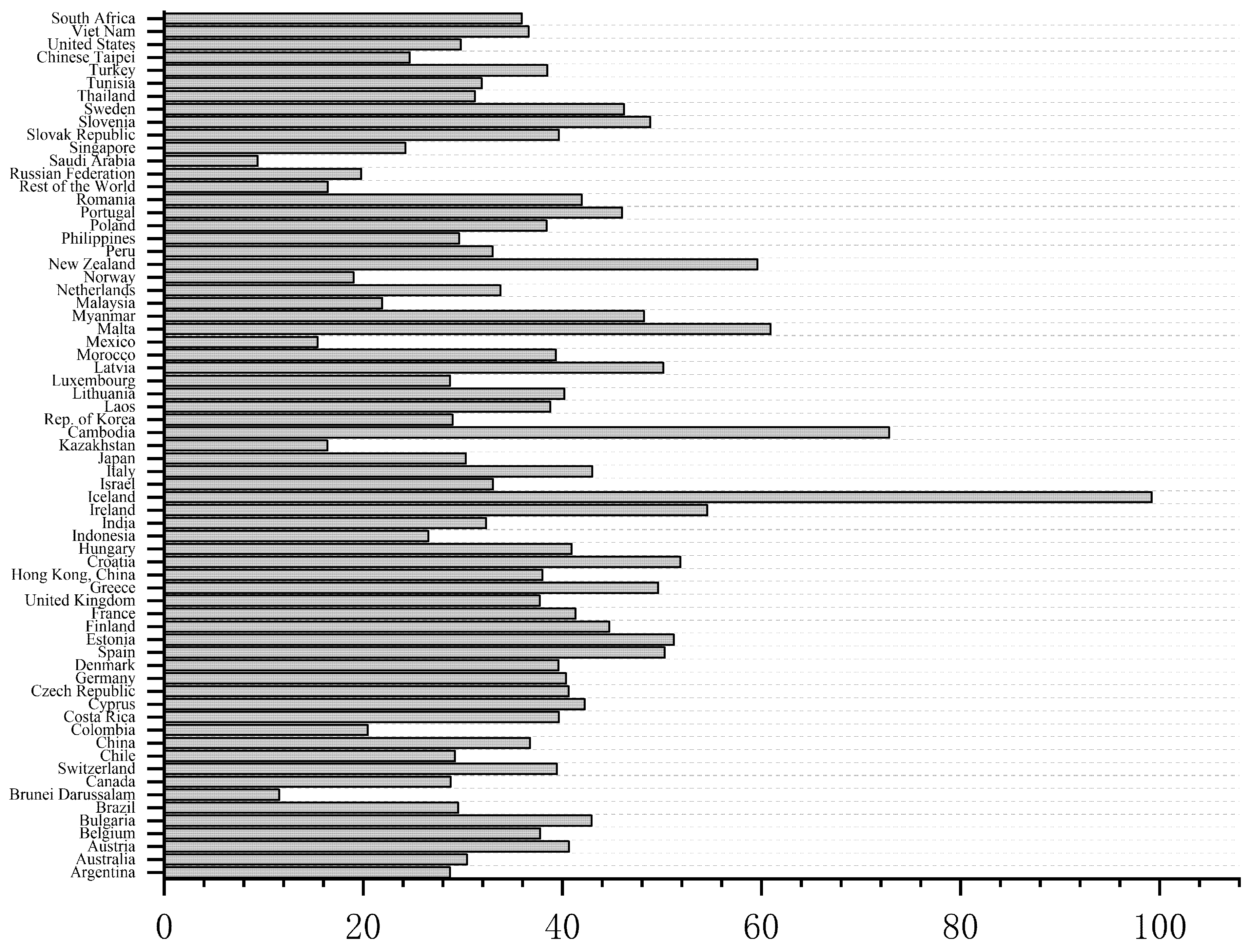
Figure 1. Forward industry average weighted degree distribution.
Sustainability 14 15138 g001
Figure 2. Backward industry average weighted degree distribution.
Sustainability 14 15138 g002
Figure 3. Heat map of similarity towards industry before 2000.
Sustainability 14 15138 g003aSustainability 14 15138 g003bSustainability 14 15138 g003c
Figure 4. The network of global carbon emission linkages in both 2000, 2018.
Sustainability 14 15138 g004
Table 1. Cycle ratio of some countries in 2000 and 2018.
ForwardBackward
2000201820002018
China4.5775.1432.6042.362
America2.6262.4732.6633.797
Germany3.4543.6652.1992.758
England3.2793.0852.8793.280
France3.9994.0743.4382.784
Japan2.4512.3451.7411.856
Korea2.4502.4331.4791.823
Russia2.3302.3443.6493.332
India3.2322.6131.5901.916
Table 2. Cycle ratio of some industries in 2000 and 2018.
ForwardBackward
2000201820002018
D01T024.2587.57828.10130.501
D2131.61027.7753.9032.048
D252.4613.4913.7064.023
D263.4013.3682.2181.591
D522.2412.1994.5935.257
D64T668.1506.0691.8491.905
D69T753.5942.7924.0123.884
D843.3724.4972.7742.813
D852.8993.3112.2182.326
Table 3. Top 10 countries with weighted indegree from 2000 to 2018.
Year12345678910
2000USAChinaJapanRussiaIndiaGermanyUKBrazilFranceItaly
2006USAChinaJapanRussiaIndiaGermanyUKBrazilFranceItaly
2012ChinaUSAIndiaRussiaJapanBrazilGermanyUKCanadaIran
2018ChinaUSAIndiaRussiaJapanBrazilGermanyIndonesiaIranSaudi Arabia
Table 4. Top 10 countries with weighted outdegree from 2000 to 2018.
Year12345678910
2000USAChinaRussiaIndiaJapanGermanyBrazilCanadaUKItaly
2006ChinaUSARussiaIndiaJapanGermanyBrazilCanadaIranUK
2012ChinaUSAIndiaRussiaJapanBrazilGermanyIndonesiaIranCanada
2018ChinaUSAIndiaRussiaJapanBrazilGermanyIranIndonesiaKorea
Table 5. Countries with closeness and betweenness both less than 1 from 2000 to 2018.
YearCountry
2000USA, UK
2006USA, UK
2012USA, UK
2018USA, UK, India, Russia, Japan, Brazil, Germany, Iran, Indonesia, Korea, Canada, France, Italy
Table 6. LMDI decomposition results.
Decomposition ResultsCarbon Intensity EffectIndustrial Structure EffectOutput Scale EffectTotal Effect
2000–2001−73,829.1611,061,657.994−726,021.657261,807.200
2001–2002−459,122.422−135,572.369927,053.464332,358.700
2002–2003−3,121,006.316863,505.9503,371,033.0641,113,533
2003–2004−3,787,544.259348,993.065458,4290.4461,145,739
2004–2005−2,869,250.837985,462.7063,036,935.9631,153,148
2005–2006−2,536,938.215131,182.7933,369,665.775963,910.400
2006–2007−2,056,612.819−945,665.7004,231,205.8591,228,927
2007–2008−580,8231.1051,994,754.8963,791,545.573−21,930.600
2008–20096,335,941.657−171,800.983−648,0871.526−31,6731
2009–2010−1,711,930.717−1,392,234.9894,903,457.5281,799,292
2010–2011−4,388,350.725417,369.9075,001,958.3841,030,978
2011–20121,337,354.530−1,245,181.575299,006.948391,179.900
2012–2013813,157.783−1,002,984.844717,527.757527,700.700
2013–20141,676,778.679−1,946,462.717709,721.570440,037.500
2014–20153,320,028.628−408,040.3052−3,408,984.098−496,996
2015–20162,191,325.161−1,647,892.727−861,325.6748−317,893
2016–2017−2,977,756.207495,530.7062285,9819.586377,594.1
2017–2018−2,822,500.756−526,70.832952,729,406.612−145,765
Table 7. LMDI contribution decomposition.
Contribution RateCarbon Intensity EffectIndustrial Structure EffectOutput Scale EffectSum
2000–2001−0.2824.055−2.7731
2001–2002−1.381−0.4082.7891
2002–2003−2.8030.7753.0271
2003–2004−3.3060.3054.0011
2004–2005−2.4880.8552.6341
2005–2006−2.6320.1363.4961
2006–2007−1.674−0.7703.4431
2007–2008264.846−90.958−172.8881
2008–2009−20.0040.54220.4621
2009–2010−0.952−0.7742.7231
2010–2011−4.2560.4054.8521
2011–20123.419−3.1830.7641
2012–20131.541−1.9011.3601
2013–20143.811−4.4231.6131
2014–2015−6.6800.8216.8591
2015–2016−6.8935.1842.7091
2016–2017−7.8861.3127.5741
2017–201819.3630.361−18.7251
Table 8. Indicator variable systems.
System VariableSubsystem VariableVariable NameVariable SymbolIndicator Sender(S) Receiver(R)
Dependent variableGlobal trade implies a carbon emissions relationshipY
Independent variableCore explanatory variableDegree of forward industry value chain embeddedGVC_IVS & R
Degree of backward industry value chain embeddedGVC_FVS & R
Network Structure Variableedgesedges
Forward industrial embedded network centralityq_eigS & R
Backward industrial embedded network centralityh_eigS & R
Control variableGDP per capita (USD)lnGDPS & R
Percentage of manufacturing value added (%)structureS & R
R&D expenditure share (%)tecS & R
GDP energy consumption per unit (USD/kg oil)energyS & R
Other covariateGeographical proximitygeo
Time-dependent variablestabilitystability
Transferabilityauto
Dischargeabilityloss
Updatabilityinnovation
Table 9. Empirical results of forward industry value chain embedded in trade implied carbon emissions.
VariablesModel 1Model 2Model 3Model 4Model 5
Structure-dependent
edges5.39 ***
(0.47)
7.62 ***
(0.70)
3.60 ***
(0.69)
3.68 ***
(0.69)
11.61 ***
(0.75)
Receiver Properties
Core explanatory
GVC_IV−1.89 ***
(0.54)
−3.20 ***
(0.70)
−3.78 ***
(0.71)
−3.08 ***
(0.69)
−3.33 ***
(0.70)
High-order structural
q_eig6.35 ***
(0.26)
9.32 ***
(0.44)
9.35 ***
(0.45)
9.07 ***
(0.45)
9.08 ***
(0.45)
Control
lnGDP0.62 ***
(0.06)
0.33 ***
(0.10)
0.39 ***
(0.10)
0.29 ***
(0.10)
0.33 ***
(0.10)
structure0.01
(0.01)
0.03 ***
(0.01)
0.04 ***
(0.01)
0.03 ***
(0.01)
0.03 ***
(0.01)
tec0.24 ***
(0.04)
0.35 ***
(0.06)
0.36 ***
(0.06)
0.40 ***
(0.06)
0.44 ***
(0.06)
energy−0.29 ***
(0.05)
−1.02 ***
(0.07)
−1.07 ***
(0.07)
−1.14 ***
(0.07)
−1.15 ***
(0.07)
Sender Properties
Core explanatory
GVC_IV−1.89 ***
(0.47)
−1.00
(0.64)
−0.82
(0.65)
−0.75
(0.65)
−1.21
(0.65)
High-order structural
q_eig−1.70 ***
(0.36)
0.14
(0.51)
0.70
(0.50)
−0.07
(0.52)
0.32
(0.52)
Control
lnGDP−0.70 ***
(0.08)
−0.52 ***
(0.12)
−0.58 ***
(0.12)
−0.62 ***
(0.12)
−0.48 ***
(0.12)
structure0.04 ***
(0.01)
0.07 ***
(0.01)
0.06 ***
(0.01)
0.06 ***
(0.01)
0.07 ***
(0.01)
tec0.56 ***
(0.05)
0.73 ***
(0.08)
0.77 ***
(0.08)
0.72 ***
(0.08)
0.70 ***
(0.08)
energy0.26 ***
(0.05)
−0.15 **
(0.07)
−0.10
(0.08)
0.01
(0.07)
−0.00
(0.07)
Covariates
geo2.22 ***
(0.47)
1.81 ***
(0.55)
1.79 ***
(0.55)
1.68 ***
(0.51)
2.27 ***
(0.66)
Time-dependent
stability 4.18 ***
(0.11)
auto 8.45 ***
(0.23)
loss −8.46 ***
(0.23)
innovation −8.38 ***
(0.23)
Num79,04074,88074,88074,88074,880
AIC2,011,966.991,796,770.081,796,625.221,796,655.591,796,659.82
BIC2,012,138.311,796,952.011,796,807.151,796,837.521,796,841.75
Note: Values in parentheses are z-values. ** indicates significant at the 5% level, and *** indicates significant at the 1% level.
Table 10. Empirical results of backward industry value chain embedded in trade implied carbon emissions.
VariablesModel 1Model 2Model 3Model 4Model 5
Structure-dependent
edges3.23 ***
(0.49)
4.45 ***
(0.70)
0.75
(0.70)
0.38
(0.70)
8.22 ***
(0.75)
Receiver Properties
Core explanatory
GVC_IV−1.93 ***
(0.25)
−0.75 **
(0.36)
−0.76 **
(0.37)
−0.53
(0.37)
−0.85 **
(0.37)
High-order structural
q_eig−2.32 ***
(0.26)
−2.07 ***
(0.44)
−1.97 ***
(0.45)
−2.01 ***
(0.45)
−1.88 ***
(0.45)
Control
lnGDP0.27 ***
(0.06)
−0.14
(0.09)
−0.21 **
(0.09)
−0.09
(0.09)
−0.15
(0.09)
structure−0.00
(0.01)
0.01
(0.01)
−0.00
(0.01)
0.00
(0.01)
−0.00
(0.01)
tec0.18 ***
(0.04)
0.28 ***
(0.05)
0.32 ***
(0.06)
0.27 ***
(0.05)
0.34 ***
(0.06)
energy−0.04
(0.04)
−0.87 ***
(0.07)
−0.91 ***
(0.07)
−0.89 ***
(0.07)
−0.92 ***
(0.07)
Sender Properties
Core explanatory
GVC_IV1.17 ***
(0.29)
0.33
(0.36)
0.47
(0.36)
0.42
(0.37)
0.87 **
(0.37)
High-order structural
q_eig−1.38 ***
(0.24)
−2.32 ***
(0.34)
−2.36 ***
(0.34)
−2.24 ***
(0.34)
−2.44 ***
(0.34)
Control
lnGDP−0.77 ***
(0.08)
−0.55 ***
(0.10)
−0.54 ***
(0.11)
−0.57 ***
(0.11)
−0.50 ***
(0.11)
structure0.05 ***
(0.01)
0.05 ***
(0.01)
0.06 ***
(0.01)
0.05 ***
(0.01)
0.05 ***
(0.01)
tec0.60 ***
(0.05)
0.63 ***
(0.07)
0.56 ***
(0.07)
0.59 ***
(0.07)
0.54 ***
(0.07)
energy0.28 ***
(0.04)
0.07
(0.07)
0.06
(0.07)
0.10
(0.07)
0.13 **
(0.07)
Covariates
geo2.02 ***
(0.47)
1.63 ***
(0.52)
1.78 ***
(0.54)
1.59 ***
(0.53)
1.78 ***
(0.54)
Time-dependent
stability 3.98 ***
(0.11)
auto 8.14 ***
(0.23)
loss −7.98 ***
(0.22)
innovation −7.98 ***
(0.22)
Num79,04074,88074,88074,88074,880
AIC2,012,021.451,797,254.391,797,126.041,797,109.471,797,091.35
BIC2,012,192.761,797,436.321,797,307.961,797,291.401,797,273.28
Note: Values in parentheses are z-values. ** indicates significant at the 5% level, and *** indicates significant at the 1% level.
Table 11. The results of extrapolation from an out-of-sample.
VariablesModel 1VariablesModel 2
Structure-dependent Structure-dependent
edges3.91 ***
(0.51)
edges2.35 ***
(0.51)
Receiver Properties Receiver Properties
Core explanatory Core explanatory
GVC_IV−2.45 ***
(0.57)
GVC_IV−1.61 ***
(0.27)
High-order structural High-order structural
q_eig4.46 ***
(0.26)
q_eig−2.16 ***
(0.28)
Control Control
lnGDP0.69 ***
(0.07)
lnGDP0.35 ***
(0.07)
structure0.01
(0.01)
structure−0.00
(0.01)
tec0.12 ***
(0.05)
tec0.13 ***
(0.04)
energy0.02
(0.05)
energy0.14 ***
(0.05)
Sender Properties Sender Properties
Core explanatory Core explanatory
GVC_IV−1.48 ***
(0.50)
GVC_IV1.20 ***
(0.31)
High-order structural High-order structural
q_eig−2.32 ***
(0.35)
q_eig−1.21 ***
(0.26)
Control Control
lnGDP−0.80 ***
(0.09)
lnGDP−0.80 ***
(0.08)
structure0.03 ***
(0.01)
structure0.04 ***
(0.01)
tec0.51 ***
(0.05)
tec0.51 ***
(0.05)
energy0.37 ***
(0.05)
energy0.38 ***
(0.05)
Covariates Covariates
geo2.18 ***
(0.50)
geo2.06 ***
(0.50)
Note: Values in parentheses are z-values. *** indicates significant at the 1% level.
Table 12. The results of Great Likelihood Estimation Using Markov Monte Carlo.
VariablesModel 1VariablesModel 2
Structure-dependent Structure-dependent
edges4.01 ***
(0.49)
edges2.16 ***
(0.49)
Receiver Properties Receiver Properties
Core explanatory Core explanatory
GVC_IV−2.27 ***
(0.54)
GVC_IV−1.71 ***
(0.54)
High-order structural High-order structural
q_eig5.18 ***
(0.23)
q_eig−2.15 ***
(0.23)
Control Control
lnGDP0.72 ***
(0.07)
lnGDP0.50 ***
(0.07)
structure0.00
(0.01)
structure−0.00
(0.01)
tec0.18 ***
(0.04)
tec0.20 ***
(0.04)
energy−0.00
(0.05)
energy0.17 ***
(0.05)
Sender Properties Sender Properties
Core explanatory Core explanatory
GVC_IV−1.45 ***
(0.64)
GVC_IV0.96 ***
(0.64)
High-order structural High-order structural
q_eig−2.32 ***
(0.33)
q_eig−1.18 ***
(0.33)
Control Control
lnGDP−0.75 ***
(0.08)
lnGDP−0.75 ***
(0.08)
structure0.03 ***
(0.01)
structure0.03 ***
(0.01)
tec0.52 ***
(0.05)
tec0.52 ***
(0.05)
energy0.35 ***
(0.05)
energy0.28 ***
(0.05)
Covariates Covariates
geo2.20 ***
(0.48)
geo2.31 ***
(0.58)
Note: Values in parentheses are z-values. *** indicates significant at the 1% level.
Publisher’s Note: MDPI stays neutral with regard to jurisdictional claims in published maps and institutional affiliations.