
Performance Evaluation of LIDAR and SODAR Wind Profilers on the Brazilian Equatorial Margin

 ,
,  , , ,
, , ,  , ,
, ,  , , , , and
Abstract
1. Introduction
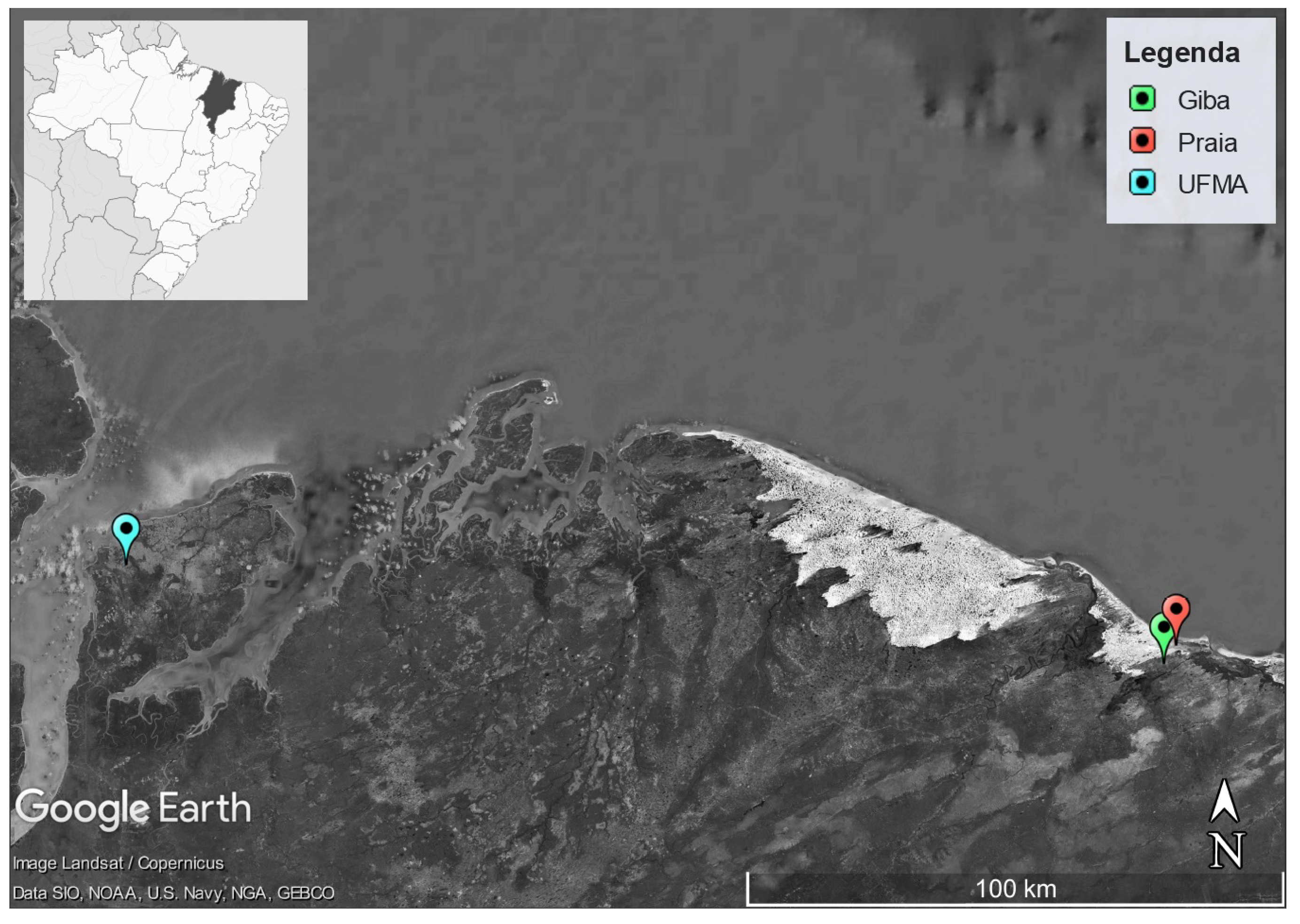
2. Measurement Campaigns: Sites and Procedures
3. Regional Climatology
- With intervals between 2 and 7 years, the atmospheric teleconnections El Niño and La Niña have impacts on global atmospheric circulation, with well-defined effects on various “climatic” patterns in Brazil, such as precipitation and wind circulation in the northeast [17,18,19,20,21,22,23,24,25,26,27,28,29,30];
4. LIDAR and SODAR Wind Profilers
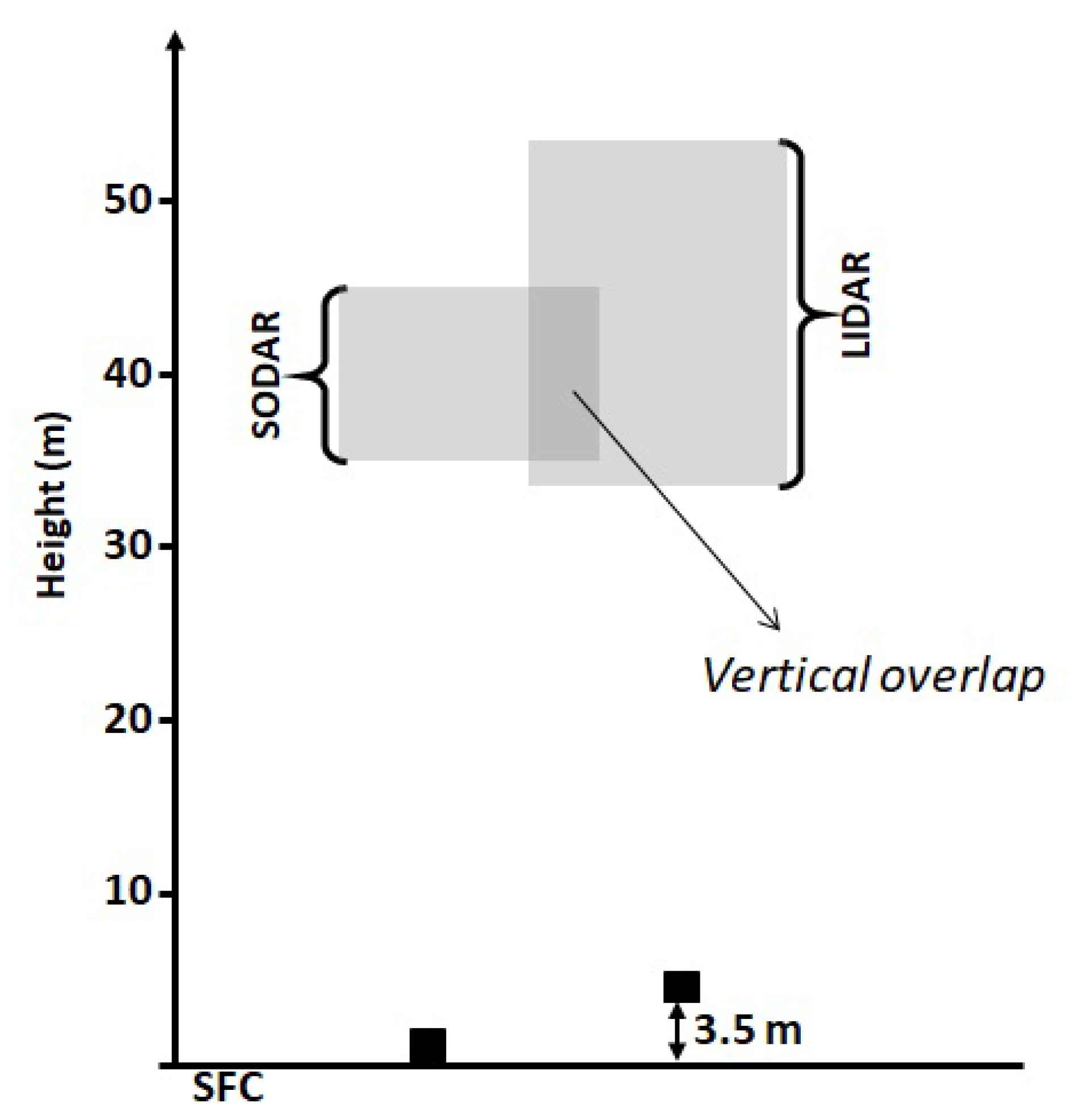
5. Methodology
- is the distance between the LIDAR and the SODAR;
- is the scanning cone angle of the LIDAR;
- is the angle of the scanning cone of SODAR;
- is the height of the LIDAR.
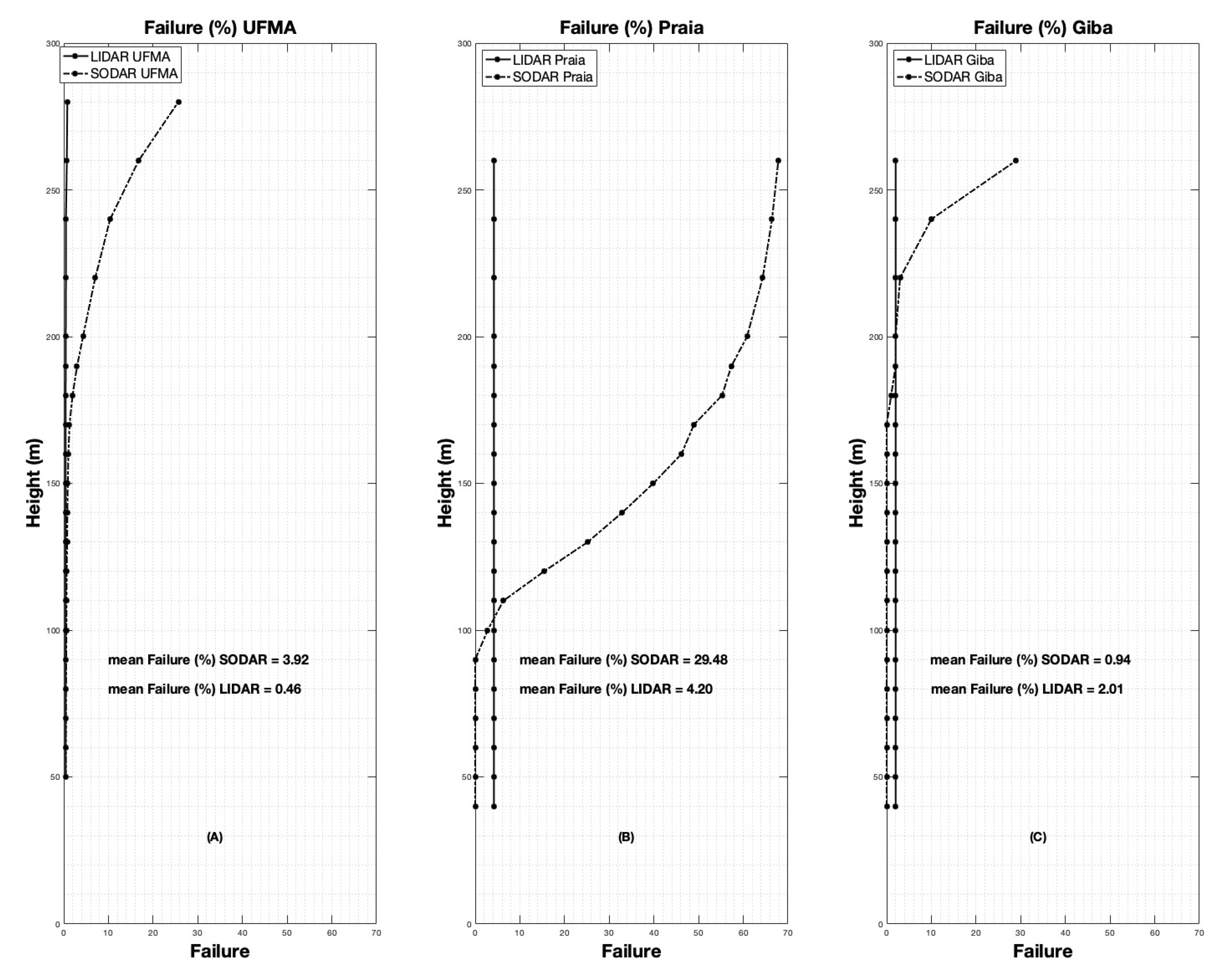
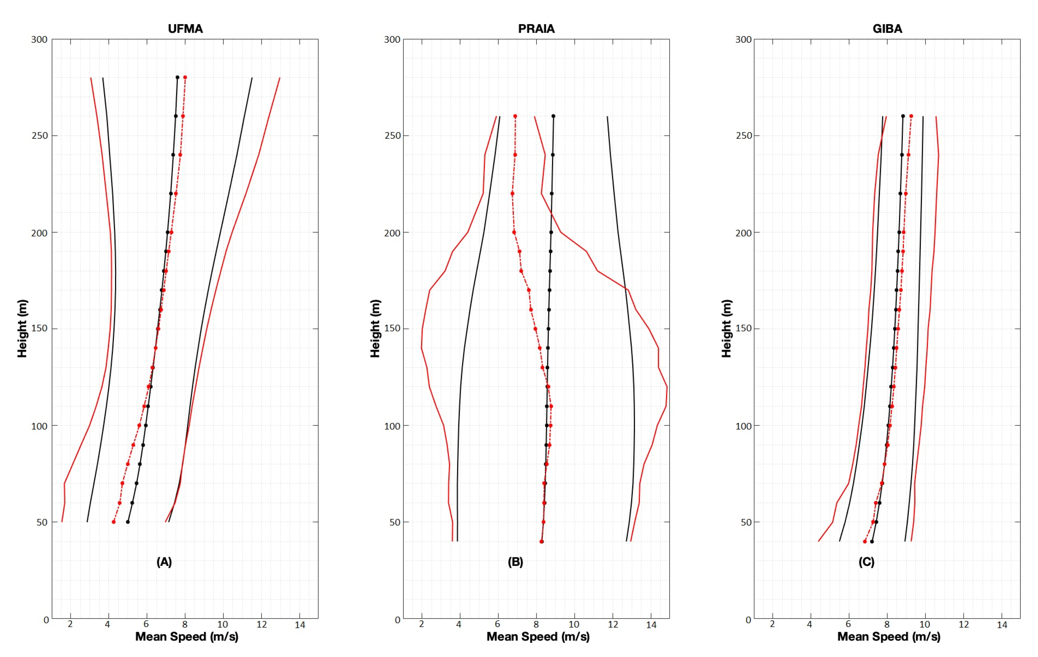
6. Results and Discussions
7. Summary and Conclusions
Author Contributions
Funding
Institutional Review Board Statement
Informed Consent Statement
Data Availability Statement
Acknowledgments
Conflicts of Interest
References
- Assireu, A.T.; Pimenta, F.M.; de Freitas, R.M.; Saavedra, O.R.; Neto, F.L.A.; Torres, A.R., Jr.; Oliveira, C.B.M.; Lopes, D.C.P.; de Lima, S.L.; Veras, R.B.S.; et al. EOSOLAR Project: Assessment of wind resources of a coastal equatorial region of Brazil—Overview and preliminary results. Energies 2022, 15, 2319. [Google Scholar] [CrossRef]
- Stickland, M.; Scanlon, T.; Fabre, S. Comparison of Zephir and Windcube measurements in the same complex flowfield. In Proceedings of the EWEA OFFSHORE 2011, Amsterdam, The Netherlands, 29 November–1 December 2011; University of Strathclyde: Glasgow, UK, 2011. [Google Scholar]
- Lang, S.; McKeogh, E. LIDAR and SODAR measurements of wind speed and direction in upland terrain for wind energy purposes. Remote Sens. 2011, 3, 1871–1901. [Google Scholar] [CrossRef]
- Antoniou, I.; Jørgensen, H.E.; Ormel, F.; Bradley, S.; von Hünerbein, S.; Emeis, S.; Warmbier, G. On the Theory of SODAR Measurement Techniques; OCLC: 473721156; Risø National Laboratory, Information Service Department: Roskilde, Denmark, 2003. [Google Scholar]
- Kallistratova, M.A.; Petenko, I.V.; Kouznetsov, R.D.; Kulichkov, S.N.; Chkhetiani, O.G.; Chunchusov, I.P.; Lyulyukin, V.S.; Zaitseva, D.V.; Vazaeva, N.V.; Kuznetsov, D.D.; et al. Sodar sounding of the atmospheric boundary layer: Review of studies at the Obukhov Institute of Atmospheric Physics, Russian Academy of Sciences. Izv. Atmos. Ocean. Phys. 2018, 54, 242–256. [Google Scholar] [CrossRef]
- Kelley, N.D.; Jonkman, B.J.; Scott, G.N.; Pichugina, Y.L. Comparing Pulsed Doppler LIDAR with SODAR and Direct Measurements for Wind Assessment; Technical Report; National Renewable Energy Lab. (NREL): Golden, CO, USA, 2007. [Google Scholar]
- Sotelino, L.G.; Coster, N.D.; Beirinckx, P.; Peeters, P. Intercomparison of Cup Anemometer and Sonic Snemometers on Site at Uccle/Belgium. In Proceedings of the WMO Technical Conference on Meteorological and Environmental Instruments and Methods of Observation (TECO-2012), Brussels, Belgium, 16–18 October 2012; p. 7. [Google Scholar]
- Dubov, D.; Aprahamian, B.; Aprahamian, M. Comparison between conventional wind measurement systems and SODAR systems for remote sensing including examination of real wind data. In Proceedings of the 2017 15th International Conference on Electrical Machines, Drives and Power Systems (ELMA), Sofia, Bulgaria, 1–3 June 2017; IEEE: Piscataway, NJ, USA, 2017; pp. 106–109. [Google Scholar] [CrossRef]
- Finn, A.; Rogers, K.; Rice, F.; Meade, J.; Holland, G.; May, P. A comparison of vertical atmospheric wind profiles obtained from monostatic Sodar and unmanned aerial vehicle–based acoustic tomography. J. Atmos. Ocean. Technol. 2017, 34, 2311–2328. [Google Scholar] [CrossRef]
- Sinha, S.; Regeena, M.L.; Sarma, T.V.C.; Hashiguchi, H.; Tuckley, K.R. Doppler Profile Tracing Using MPCF on MU Radar and Sodar: Performance Analysis. IEEE Geosci. Remote Sens. Lett. 2018, 15, 508–511. [Google Scholar] [CrossRef]
- Buzdugan, L.; Stefan, S. A comparative study of SODAR, LIDAR wind measurements and aircraft derived wind observations. Rom. J. Phys. 2020, 65, 810. [Google Scholar]
- Buzdugan, L.; Bugeac, O.P.; Stefan, S. A comparison of low-level wind profiles from Mode-S EHS data with ground-based remote sensing data. Meteorol. Atmos. Phys. 2021, 133, 1455–1468. [Google Scholar] [CrossRef]
- Zhou, Z.; Bu, Z. Wind measurement comparison of Doppler lidar with wind cup and L band sounding radar. Atmos. Meas. Tech. Discuss. 2021, preprint. [Google Scholar] [CrossRef]
- Aitken, M.L.; Rhodes, M.E.; Lundquist, J.K. Performance of a Wind-Profiling Lidar in the Region of Wind Turbine Rotor Disks. J. Atmos. Ocean. Technol. 2012, 29, 347–355. [Google Scholar] [CrossRef]
- Kumer, V.M.; Reuder, J.; Furevik, B.R. A Comparison of LiDAR and Radiosonde Wind Measurements. Energy Procedia 2014, 53, 214–220. [Google Scholar] [CrossRef]
- Alfredini, P.; Arasaki, E.; Fortner, E. Behavior of sea level in the period of 1980 to 2017 on the port area of Gulf of Maranhão, Brazil. Transnav Int. J. Mar. Navig. Saf. Sea Transp. 2021, 15, 683–686. [Google Scholar] [CrossRef]
- Philander, S.G.H. El Niño Southern Oscillation phenomena. Nature 1983, 302, 295–301. [Google Scholar] [CrossRef]
- Philander, S.; Seigel, A. Chapter 33 Simulation of El Niño of 1982–1983. In Deep Sea Research Part II: Topical Studies in Oceanography; Elsevier: Amsterdam, The Netherlands, 1985; Volume 40, pp. 517–541. [Google Scholar] [CrossRef]
- Philander, S.G.; Rasmusson, E.M. The Southern Oscillation and El Niño. In Advances in Geophysics; Elsevier: Amsterdam, The Netherlands, 1985; Volume 28, pp. 197–215. [Google Scholar] [CrossRef]
- Philander, G. El Niño and La Niña. Am. Sci. 1989, 77, 451–459. [Google Scholar]
- Kane, R.P. Prediction of Droughts in North-East Brazil: Role of ENSO and Use of Periodicities. Int. J. Climatol. 1997, 17, 655–665. [Google Scholar] [CrossRef]
- Goddard, L.; Philander, S.G. The Energetics of El Niño and La Niña. J. Clim. 2000, 13, 1496–1516. [Google Scholar] [CrossRef]
- Grimm, A.M. The El Niño Impact on the Summer Monsoon in Brazil: Regional Processes versus Remote Influences. J. Clim. 2003, 16, 263–280. [Google Scholar] [CrossRef]
- Philander, S.G.; Fedorov, A. Is El Niño Sporadic or Cyclic? Annu. Rev. Earth Planet. Sci. 2003, 31, 579–594. [Google Scholar] [CrossRef]
- Hastenrath, S. Circulation and teleconnection mechanisms of Northeast Brazil droughts. Prog. Oceanogr. 2006, 70, 407–415. [Google Scholar] [CrossRef]
- Philander, S.G. Our Affair with El Nino: How We Transformed an Enchanting Peruvian Current Into a Global Climate Hazard; Princeton University Press: Princeton, NJ, USA, 2006. [Google Scholar]
- Kayano, M.T.; Andreoli, R.V. Relationships between rainfall anomalies over northeastern Brazil and the El Niño–Southern Oscillation. J. Geophys. Res. 2006, 111, D13101. [Google Scholar] [CrossRef]
- Rodrigues, R.R.; Haarsma, R.J.; Campos, E.J.D.; Ambrizzi, T. The Impacts of Inter–El Niño Variability on the Tropical Atlantic and Northeast Brazil Climate. J. Clim. 2011, 24, 3402–3422. [Google Scholar] [CrossRef]
- Cai, W.; McPhaden, M.J.; Grimm, A.M.; Rodrigues, R.R.; Taschetto, A.S.; Garreaud, R.D.; Dewitte, B.; Poveda, G.; Ham, Y.G.; Santoso, A.; et al. Climate impacts of the El Niño–Southern Oscillation on South America. Nat. Rev. Earth Environ. 2020, 1, 215–231. [Google Scholar] [CrossRef]
- Costa, M.d.S.; Oliveira-Júnior, J.F.d.; Santos, P.J.d.; Correia Filho, W.L.F.; Gois, G.d.; Blanco, C.J.C.; Teodoro, P.E.; Silva Junior, C.A.d.; Santiago, D.d.B.; Souza, E.d.O.; et al. Rainfall extremes and drought in Northeast Brazil and its relationship with El Niño–Southern Oscillation. Int. J. Climatol. 2021, 41, 6835. [Google Scholar] [CrossRef]
- Glenn, A.H. Circulation and Convergence in the Equatorial Zone Between 95∘ E and 160∘ E: December to February*. Bull. Am. Meteorol. Soc. 1947, 28, 453–464. [Google Scholar] [CrossRef]
- Simpson, R.H. Synoptic Aspects of the Intertropical Convergence Near Central and South America. Bull. Am. Meteorol. Soc. 1947, 28, 335–346. [Google Scholar] [CrossRef]
- Miles, M.K. Meteorology. Sci. Prog. (1933) 1948, 36, 86–101. [Google Scholar]
- Crowe, P.R. The seasonal variation in the strength of the trades. In Transactions and Papers (Institute of British Geographers); Wiley: Hoboken, NJ, USA, 1950; p. 25. [Google Scholar] [CrossRef]
- Waliser, D.E.; Somerville, R.C.J. Preferred latitudes of the Intertropical Convergence Zone. J. Atmos. Sci. 1994, 51, 1619–1639. [Google Scholar] [CrossRef]
- Philander, S.G.H.; Gu, D.; Lambert, G.; Li, T.; Halpern, D.; Lau, N.C.; Pacanowski, R.C. Why the ITCZ Is Mostly North of the Equator. J. Clim. 1996, 9, 2958–2972. [Google Scholar] [CrossRef]
- Gomes, H.B.; Ambrizzi, T.; Herdies, D.L.; Hodges, K.; Pontes da Silva, B.F. Easterly Wave Disturbances over Northeast Brazil: An Observational Analysis. Adv. Meteorol. 2015, 2015, 176238. [Google Scholar] [CrossRef]
- Waliser, D.; Jiang, X. Tropical meteorology and climate: Intertropical Convergence Zone. In Encyclopedia of Atmospheric Sciences; Elsevier: Amsterdam, The Netherlands, 2015; pp. 121–131. [Google Scholar] [CrossRef]
- Nogués-Paegle, J.; Mechoso, C.R.; Fu, R.; Berbery, E.H.; Chao, W.C.; Chen, T.C.; Cook, K.; Diaz, A.F.; Enfield, D.; Ferreira, R.; et al. Progress in Pan American CLIVAR research: Understanding the South American monsoon. Meteorologica 2002, 27, 1–30. [Google Scholar]
- Gan, M.A.; Kousky, V.E.; Ropelewski, C.F. The South America Monsoon Circulation and Its Relationship to Rainfall over West-Central Brazil. J. Clim. 2004, 17, 47–66. [Google Scholar] [CrossRef]
- Liebmann, B.; Mechoso, C.R. The South American Monsoon System. In World Scientific Series on Asia-Pacific Weather and Climate, 2nd ed.; World Scientific: Singapore, 2011; Volume 5, pp. 137–157. [Google Scholar] [CrossRef]
- Marengo, J.A.; Liebmann, B.; Grimm, A.M.; Misra, V.; Silva Dias, P.L.; Cavalcanti, I.F.A.; Carvalho, L.M.V.; Berbery, E.H.; Ambrizzi, T.; Vera, C.S.; et al. Recent developments on the South American monsoon system: Recent Developments on the South American Monsoon System. Int. J. Climatol. 2012, 32, 1–21. [Google Scholar] [CrossRef]
- Vuille, M.; Burns, S.J.; Taylor, B.L.; Cruz, F.W.; Bird, B.W.; Abbott, M.B.; Kanner, L.C.; Cheng, H.; Novello, V.F. A review of the South American monsoon history as recorded in stable isotopic proxies over the past two millennia. Clim. Past 2012, 8, 1309–1321. [Google Scholar] [CrossRef]
- de Carvalho, L.M.V.; Cavalcanti, I.F.A. The South American Monsoon System (SAMS). In The Monsoons and Climate Change; de Carvalho, L.M.V., Jones, C., Eds.; Springer Climate; Springer International Publishing: Cham, Switzerland, 2016; pp. 121–148. [Google Scholar] [CrossRef]
- Correa, I.C.; Arias, P.A.; Rojas, M. Evaluation of multiple indices of the South American monsoon. Int. J. Climatol. 2021, 41, E2801–E2819. [Google Scholar] [CrossRef]
- Madden, R.A.; Julian, P.R. Detection of a 40–50 Day Oscillation in the Zonal Wind in the Tropical Pacific. J. Atmos. Sci. 1971, 28, 702–708. [Google Scholar] [CrossRef]
- Madden, R.A.; Julian, P.R. Description of Global-Scale Circulation Cells in the Tropics with a 40–50 Day Period. J. Atmos. Sci. 1972, 29, 1109–1123. [Google Scholar] [CrossRef]
- Madden, R.A.; Julian, P.R. Observations of the 40–50-Day Tropical Oscillation—A Review. Mon. Weather. Rev. 1994, 122, 814–837. [Google Scholar] [CrossRef]
- de Souza, E.B.; Ambrizzi, T. Modulation of the intraseasonal rainfall over tropical Brazil by the Madden–Julian oscillation. Int. J. Climatol. 2006, 26, 1759–1776. [Google Scholar] [CrossRef]
- Alvarez, M.S.; Vera, C.S.; Kiladis, G.N.; Liebmann, B. Influence of the Madden Julian Oscillation on precipitation and surface air temperature in South America. Clim. Dyn. 2016, 46, 245–262. [Google Scholar] [CrossRef]
- Mayta, V.C.; Ambrizzi, T.; Espinoza, J.C.; Silva Dias, P.L. The role of the Madden-Julian oscillation on the Amazon Basin intraseasonal rainfall variability. Int. J. Climatol. 2019, 39, 343–360. [Google Scholar] [CrossRef]
- Mayta, V.C.; Silva, N.P.; Ambrizzi, T.; Dias, P.L.S.; Espinoza, J.C. Assessing the skill of all-season diverse Madden–Julian oscillation indices for the intraseasonal Amazon precipitation. Clim. Dyn. 2020, 54, 3729–3749. [Google Scholar] [CrossRef]
- Zhang, C.; Adames, A.F.; Khouider, B.; Wang, B.; Yang, D. Four theories of the Madden-Julian Oscillation. Rev. Geophys. 2020, 58, e2019RG000685. [Google Scholar] [CrossRef]
- Vasconcelos Junior, F.d.C.; Jones, C.; Gandu, A.W.; Martins, E.S.P.R. Impacts of the Madden-Julian Oscillation on the intensity and spatial extent of heavy precipitation events in northern Northeast Brazil. Int. J. Climatol. 2021, 41, 3628–3639. [Google Scholar] [CrossRef]
- Sena, A.C.T.; Peings, Y.; Magnusdottir, G. Effect of the Quasi-Biennial Oscillation on the Madden Julian Oscillation Teleconnections in the Southern Hemisphere. Geophys. Res. Lett. 2022, 49, e2021GL096105. [Google Scholar] [CrossRef]
- Serra, Y.L.; Kiladis, G.N.; Cronin, M.F. Horizontal and Vertical Structure of Easterly Waves in the Pacific ITCZ. J. Atmos. Sci. 2008, 65, 1266–1284. [Google Scholar] [CrossRef]
- Toma, V.E.; Webster, P.J. Oscillations of the Intertropical Convergence Zone and the genesis of easterly waves. Part I: Diagnostics and theory. Clim. Dyn. 2010, 34, 587–604. [Google Scholar] [CrossRef]
- Toma, V.E.; Webster, P.J. Oscillations of the Intertropical Convergence Zone and the genesis of easterly waves Part II: Numerical verification. Clim. Dyn. 2010, 34, 605–613. [Google Scholar] [CrossRef]
- Xie, S.P.; Carton, J.A. Tropical atlantic variability: Patterns, mechanisms, and impacts. In Geophysical Monograph Series; Wang, C., Xie, S., Carton, J., Eds.; American Geophysical Union: Washington, DC, USA, 2013; pp. 121–142. [Google Scholar] [CrossRef]
- Gomes, H.B.; Ambrizzi, T.; Pontes da Silva, B.F.; Hodges, K.; Silva Dias, P.L.; Herdies, D.L.; Silva, M.C.L.; Gomes, H.B. Climatology of easterly wave disturbances over the tropical South Atlantic. Clim. Dyn. 2019, 53, 1393–1411. [Google Scholar] [CrossRef]
- de Medeiros, F.J.; de Oliveira, C.P.; Torres, R.R. Climatic aspects and vertical structure circulation associated with the severe drought in Northeast Brazil (2012–2016). Clim. Dyn. 2020, 55, 2327–2341. [Google Scholar] [CrossRef]
- Roxburgh, W. XLVII. On the land winds of Coromandel, and their causes. The Philosophical Magazine, 1 October 1810; Volume 36, pp. 243–253. [Google Scholar] [CrossRef]
- Hall, F. XXIII. Meteorological observations made during a residence in Colombia between the years 1820 and 1830. London Edinburgh Dublin Philos. Mag. J. Sci. 1838, 12, 148–158. [Google Scholar] [CrossRef][Green Version]
- Hopkins, T. LXVIII. On the diurnal change of the aqueous portion of the atmosphere, and their effects on the barometer. London Edinburgh Dublin Philos. Mag. J. Sci. 1845, 27, 427–435. [Google Scholar] [CrossRef]
- Sabine. VIII. On some points in the meteorology of Bombay. London Edinburgh Dublin Philos. Mag. J. Sci. 1846, 28, 24–35. [Google Scholar] [CrossRef]
- Kousky, V.E. Diurnal rainfall variation in northeast Brazil. Mon. Weather. Rev. 1980, 108, 488–498. [Google Scholar] [CrossRef]
- Planchon, O.; Damato, F.; Dubreuil, V.; Gouery, P. A method of identifying and locating sea-breeze fronts in north-eastern Brazil by remote sensing. Meteorol. Appl. 2006, 13, 225. [Google Scholar] [CrossRef]
- Souza, D.C.d.; Oyama, M.D. Breeze potential along the brazilian northern and northeastern coast. J. Aerosp. Technol. Manag. 2017, 9, 368–378. [Google Scholar] [CrossRef]
- Ribeiro, F.N.; Oliveira, A.P.d.; Soares, J.; Miranda, R.M.d.; Barlage, M.; Chen, F. Effect of sea breeze propagation on the urban boundary layer of the metropolitan region of Sao Paulo, Brazil. Atmos. Res. 2018, 214, 174–188. [Google Scholar] [CrossRef]
- Anjos, M.; Lopes, A. Sea breeze front identification on the northeastern coast of Brazil and its implications for meteorological conditions in the Sergipe region. Theor. Appl. Climatol. 2019, 137, 2151–2165. [Google Scholar] [CrossRef]
- Anjos, M.; Lopes, A.; Lucena, A.J.d.; Mendonça, F. Sea breeze front and outdoor thermal comfort during summer in northeastern Brazil. Atmosphere 2020, 11, 1013. [Google Scholar] [CrossRef]
- Wang, L.; Qiang, W.; Xia, H.; Wei, T.; Yuan, J.; Jiang, P. Robust solution for boundary layer height detections with coherent doppler wind lidar. Adv. Atmos. Sci. 2021, 38, 1920–1928. [Google Scholar] [CrossRef]
- LEOSPHERE. Windcube FCR Measurements; LEOSPHERE: Saclay, France, 2017. [Google Scholar]
- ScintecAG. Scintec Flat Array Sodars—Theory Manual (SFAS, MFAS, XFAS) Including RASS RAE1 and WindRASS, Version 1.03 ed; Technical Report; ScintecAG: Princeton, NJ, USA, 2017. [Google Scholar]
- Kelberlau, F.; Mann, J. Cross-contamination effect on turbulence spectra from Doppler beam swinging wind lidar. Wind. Energy Sci. 2020, 5, 519–541. [Google Scholar] [CrossRef]
- Chatfield, C. The Analysis of Time Series: An Introduction, 6th ed.; OCLC: 880737910; Taylor and Francis: Hoboken, NJ, USA, 2013. [Google Scholar]
- Bertrand, C.; González Sotelino, L.; Journée, M. Quality control of the RMI’s AWS wind observations. Adv. Sci. Res. 2016, 13, 13–19. [Google Scholar] [CrossRef]
- Lo Feudo, T.; Calidonna, C.R.; Avolio, E.; Sempreviva, A.M. Study of the vertical structure of the coastal boundary layer integrating surface measurements and ground-based remote sensing. Sensors 2020, 20, 6516. [Google Scholar] [CrossRef] [PubMed]
- Barantiev, D.; Batchvarova, E. Wind speed profile statistics from acoustic soundings at a black sea coastal site. Atmosphere 2021, 12, 1122. [Google Scholar] [CrossRef]


| Campaigns | Period | No. of Days | Location | Sea Distance |
|---|---|---|---|---|
| UFMA 1 | 7 August 2021, 12:00:01 a.m. to 26 August 2021, 11:50:01 p.m. | 20 | IEE-UFMA (2.560° S, 44.307° W) | 4–8 km |
| Praia | 9 November 2021, 2:10:01 p.m. to 10 November 2021, 1:50:01 p.m. | 20 | Near the beach (2.694° S, 42.555° W) | 1.3 km |
| Giba | 10 November 2021, 5:20:01 p.m. to 12 Novemebr 2021, 10:40:01 a.m. | 01 | Mr. Gilberto Porto’s farm (2.725° S, 42.575° W) | 5.6 km |
| Height (m) | Linear Overlap (m) | LIDAR + SODAR | Overlap or Total |
|---|---|---|---|
| 50 | 38 | 108 | 35.2% |
| 60 | 49 | 130 | 37.7% |
| 70 | 60 | 152 | 39.5% |
| 80 | 71 | 174 | 40.8% |
| 90 | 82 | 195 | 42.1% |
| 100 | 93 | 217 | 42.9% |
| 110 | 104 | 239 | 43.5% |
| 120 | 115 | 261 | 44.1% |
| 130 | 126 | 282 | 44.7% |
| 140 | 137 | 304 | 45.1% |
| 150 | 148 | 326 | 45.4% |
| 160 | 159 | 347 | 45.8% |
| 170 | 170 | 369 | 46.1% |
| 180 | 181 | 391 | 46.3% |
| 190 | 192 | 413 | 46.5% |
| 200 | 203 | 434 | 46.8% |
| 220 | 226 | 478 | 47.3% |
| 240 | 248 | 521 | 47.6% |
| 260 | 270 | 565 | 47.8% |
| 280 | 292 | 608 | 48.0% |
| UFMA | Praia | Giba | Mean | |
|---|---|---|---|---|
| Zonal | 0.99 | 0.92 | 0.94 | 0.95 |
| Meridional | 0.98 | 0.98 | 0.98 | 0.98 |
| Vertical | 0.81 | 0.77 | 0.77 | 0.78 |
| Mean | 0.93 | 0.89 | 0.90 |
| UFMA | Praia | Giba | Mean | |
|---|---|---|---|---|
| Zonal | 0.98 | 0.95 | 0.95 | 0.96 |
| Meridional | 0.97 | 0.98 | 0.99 | 0.98 |
| Vertical | 0.77 | 0.74 | 0.74 | 0.75 |
| Mean | 0.91 | 0.89 | 0.89 |
| UFMA | Praia | Giba | Mean | |
|---|---|---|---|---|
| Zonal | 0.99 | 0.88 | 0.93 | 0.93 |
| Meridional | 0.99 | 0.98 | 0.98 | 0.98 |
| Vertical | 0.85 | 0.80 | 0.81 | 0.82 |
| Mean | 0.94 | 0.89 | 0.91 |
Publisher’s Note: MDPI stays neutral with regard to jurisdictional claims in published maps and institutional affiliations. |
© 2022 by the authors. Licensee MDPI, Basel, Switzerland. This article is an open access article distributed under the terms and conditions of the Creative Commons Attribution (CC BY) license (https://creativecommons.org/licenses/by/4.0/).
Share and Cite
Torres Junior, A.R.; Saraiva, N.P.; Assireu, A.T.; Neto, F.L.A.; Pimenta, F.M.; de Freitas, R.M.; Saavedra, O.R.; Oliveira, C.B.M.; Lopes, D.C.P.; de Lima, S.L.; et al. Performance Evaluation of LIDAR and SODAR Wind Profilers on the Brazilian Equatorial Margin. Sustainability 2022, 14, 14654. https://doi.org/10.3390/su142114654
Torres Junior AR, Saraiva NP, Assireu AT, Neto FLA, Pimenta FM, de Freitas RM, Saavedra OR, Oliveira CBM, Lopes DCP, de Lima SL, et al. Performance Evaluation of LIDAR and SODAR Wind Profilers on the Brazilian Equatorial Margin. Sustainability. 2022; 14(21):14654. https://doi.org/10.3390/su142114654
Chicago/Turabian StyleTorres Junior, Audalio R., Natália P. Saraiva, Arcilan T. Assireu, Francisco L. A. Neto, Felipe M. Pimenta, Ramon M. de Freitas, Osvaldo R. Saavedra, Clóvis B. M. Oliveira, Denivaldo C. P. Lopes, Shigeaki L. de Lima, and et al. 2022. "Performance Evaluation of LIDAR and SODAR Wind Profilers on the Brazilian Equatorial Margin" Sustainability 14, no. 21: 14654. https://doi.org/10.3390/su142114654
APA StyleTorres Junior, A. R., Saraiva, N. P., Assireu, A. T., Neto, F. L. A., Pimenta, F. M., de Freitas, R. M., Saavedra, O. R., Oliveira, C. B. M., Lopes, D. C. P., de Lima, S. L., Veras, R. B. S., & Oliveira, D. Q. (2022). Performance Evaluation of LIDAR and SODAR Wind Profilers on the Brazilian Equatorial Margin. Sustainability, 14(21), 14654. https://doi.org/10.3390/su142114654