Utilities of Artificial Intelligence in Poverty Prediction: A Review

Abstract

Artificial Intelligence (AI) is generating new horizons in one of the biggest challenges in the world’s society—poverty. Our goal is to investigate utilities of AI in poverty prediction via finding answers to the following research questions: (1) How many papers on utilities of AI in poverty prediction were published up until March, 2022? (2) Which approach to poverty was applied when AI was used for poverty prediction? (3) Which AI methods were applied for predicting poverty? (4) What data were used for poverty prediction via AI? (5) What are the advantages and disadvantages of the created AI models for poverty prediction? In order to answer these questions, we selected twenty-two papers using appropriate keywords and the exclusion criteria and analyzed their content. The selection process identified that, since 2016, publications on AI applications in poverty prediction began. Results of our research illustrate that, during this relatively short period, the application of AI in predicting poverty experienced a significant progress. Overall, fifty-seven AI methods were applied during the analyzed span, among which the most popular one was random forest. It was revealed that with the adoption of AI tools, the process of poverty prediction has become, from one side, quicker and more accurate and, from another side, more advanced due to the creation and possibility of using different datasets. The originality of this work is that this is the first sophisticated survey of AI applications in poverty prediction.

1. Introduction

At the beginning of its emergence, AI was considered as a tool completely related to the IT sphere; then, AI started being used widely in various fields to find solutions to different types of problems. The economic sphere is no exception. AI tools have already been commenced widely, and it is applied in predicting economic growth [1,2], enhancing developments in agriculture spheres [3,4], stock market predictions [5], etc. The application of AI tools has not bypassed the poverty prediction field.

Poverty is a phenomenon that does not have one unique definition. There are various approaches in defining and measuring poverty, but in general, all of them can be divided into two large groups: monetary and non-monetary approaches [6,7]. The first and most widespread approach in poverty measurement is using a monetary approach: People are considered poor when they do not have enough money to maintain their livelihood [8]. In other words, poverty is measured by money: how much they earn or spend. In many countries as well as international organisations, poverty is measured using monetary approaches [9]. However, the thesis of classifying poverty as only a money issue called into questions many researchers who afterwards developed approaches to defining poverty. They claimed that poverty comprises a lack of opportunities, education, healthcare, and so on [10,11,12]. Now, more and more researchers agree that poverty is a multidimensional phenomenon that cannot be explained only by money. In order to measure and predict poverty, various data started being applied to find a more precise definition of poverty. Different models have been created to find a universal model that could be effective in all countries equally; however, models that were effective in one country can be ineffective in other countries due to economical, social, and cultural discrepancies among countries [13].

In order to measure and predict poverty rates, different econometric tools have been applied: correlation analysis, regression analysis, factor analysis, panel data analysis, and time series analysis. Since 2016, the integration of AI tools into the poverty prediction field commenced [14]. Mainly, two major sub-classes of AI have been applied in poverty analysis: machine learning and deep learning. In early papers, AI models of poverty prediction were compared with econometric models to find out whether AI can be applied in this sphere [13,15,16]. After obtaining persuasive results about the effectiveness of AI models, as the next stage, different AI models were compared with each other to select the best model [17,18]. The strengths of AI models compared with econometric models are that they can deal with the multicollinearity issue, they have higher accuracy levels, higher calculation speeds, can work with big data, and require less human involvement [19,20].

In poverty prediction processes, AI tools are applied not only for prediction itself but also for feature selection. Feature selection is also an important process in poverty prediction, which implies selecting variables that can explain poverty [13]. In selecting variables, the significance level of variable’s effect on poverty is analyzed, and the variables with high impact are selected to create models with them [15]. It is revealed that models with few but important variables can have higher accuracy levels [17]. In addition, creating models with only a few variables will also make it easy to collect data for analysis and the analysis process itself. Before AI applications, econometric tools such as stepwise, LASSO, and PCA analyses were applied for feature selection [21].

One of the benefits of AI tools is that different datasets can now be used in poverty prediction. Traditional datasets of poverty analysis are survey and census data. Yet, only they are not enough for defining poverty from various dimensions; thus, currently, remote sensing data, call detail records, and e-commerce data have started being applied in poverty prediction due to the capacity of AI applications in the extraction of necessary variables for analyses [22].

In a relatively short span, AI tools have already been widely applied in poverty prediction around the world. Although there are surveys conducted on explainable AI [23], AI applications in drought assessment [24], the impact of AI on sustainability [6,25], and health systems in resource-poor settings [26], to our knowledge, there is no comprehensive survey that includes the available literature on utilities of AI in poverty prediction. Our aim is to fill this gap by providing with an overview about the progress of AI application in poverty prediction, as well as familiarizing the created AI poverty prediction models and their outcomes. Therefore, we set the following research questions, answers to which will provide to reach our aim of writing this paper:

1.

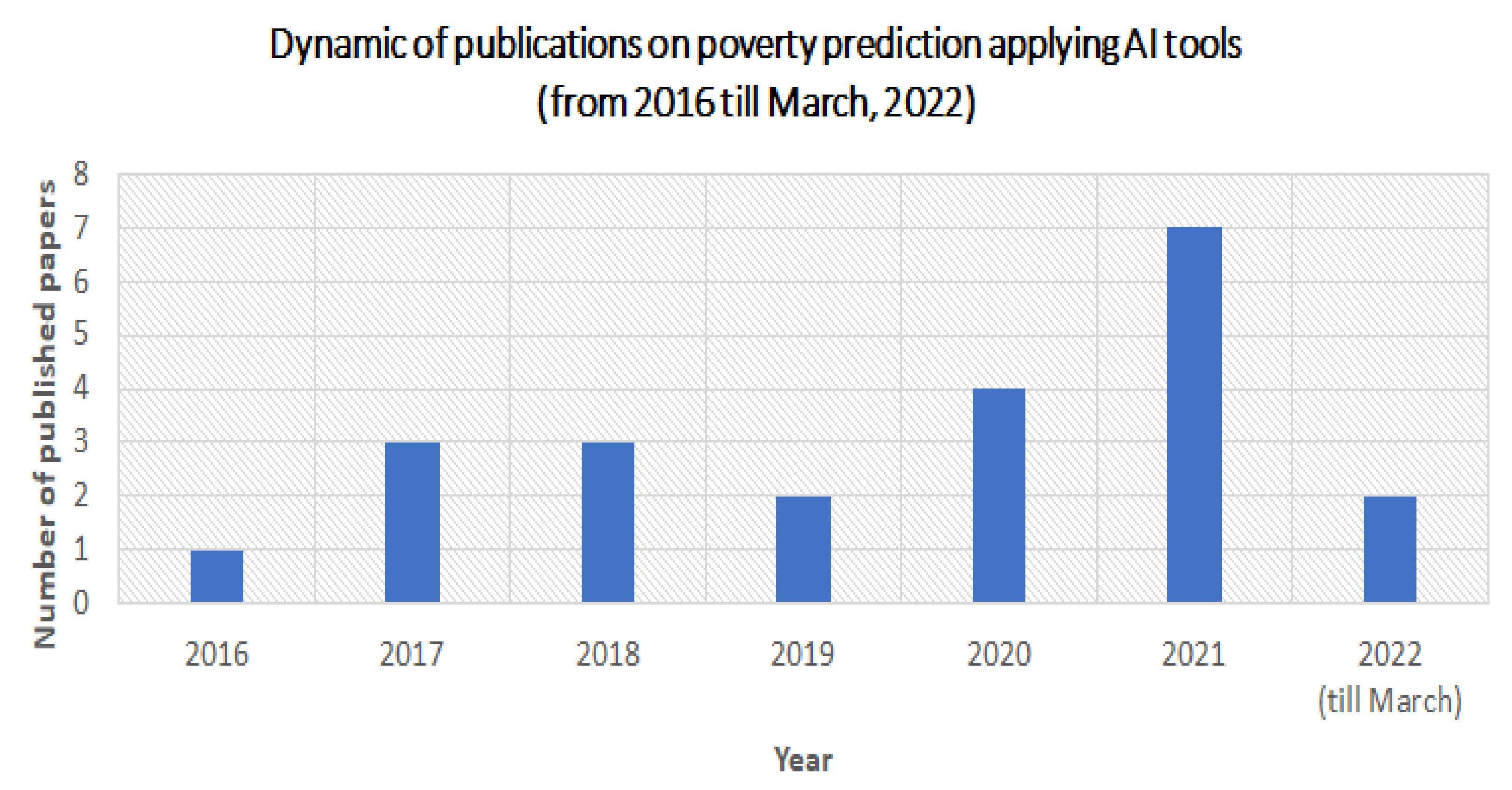
How many papers on utilities of AI in poverty prediction were published up until March 2022?

2.

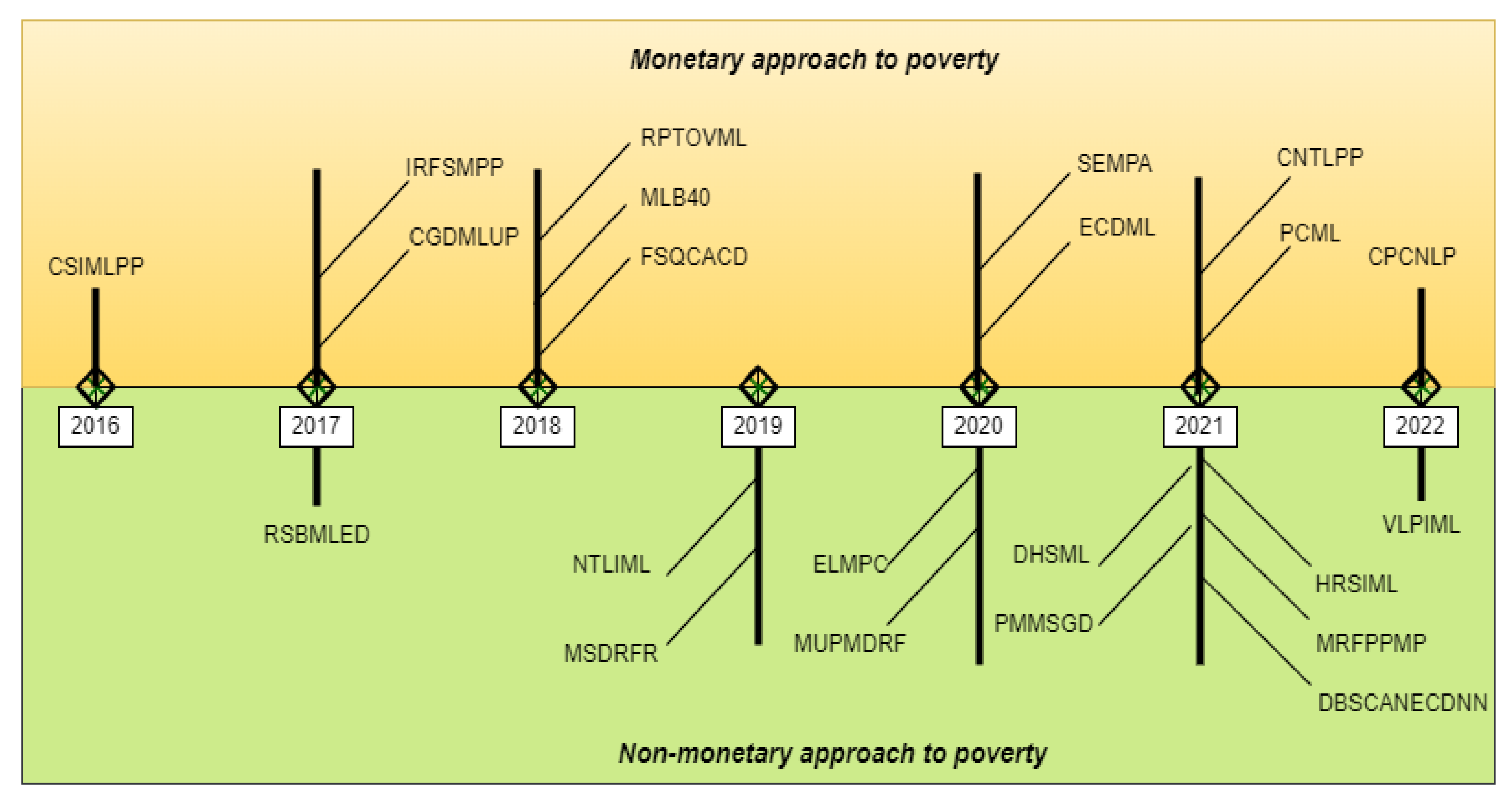
Which approach to poverty was applied when AI was used for poverty prediction?

3.

Why AI methods were applied in poverty prediction?

4.

Whether reviews on AI utilities in poverty prediction conducted before?

5.

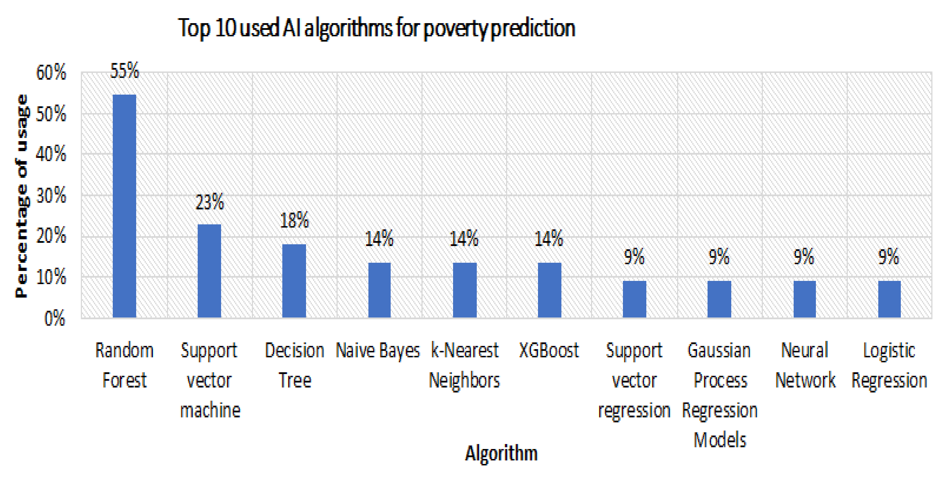
Which AI methods were applied for predicting poverty?

6.

What data were used for poverty prediction via AI?

7.

What are the advantages and disadvantages of the created AI models for poverty prediction?

8.

What is the future scope of AI applications in poverty prediction?

The rest of the article is structured as follows: Section 2 investigates and compares previously conducted reviews and surveys on applications of AI in poverty prediction. Section 3 describes details of research methodology, whereas Section 4 introduces different AI algorithms applied in poverty prediction. Section 5 makes comparisons between poverty prediction models, and the final Section 6 draws concluding remarks on utilities of AI in poverty prediction and highlights future research directions.

2. Related Reviews

Related literature reviews have two directions. In the first direction, the impact of AI on poverty was analyzed mainly in the context of providing sustainability [27,28,29]. The second direction includes review papers on AI applications in poverty measurements [27,30,31]. The overall information on previously published surveys and reviews related to AI in poverty prediction are illustrated in

Table 1. Surveys and Reviews Related to AI in Poverty Prediction.

Ref.	Year	Area of Study	Contribution	Limitations
[30]	2016	AI in poverty measurement	Discussed data used for poverty prediction with a focus on [14] work	The paper focused on data types and analyses with less attention on machine learning methods.
[31]	2020	AI in poverty measurement	Summarized information on AI methods applied in poverty measurement. In the paper, information on data and applied algorithms for poverty measurement were provided.	This work provided aggregated information about fifteen reviewed papers without in-depth analyses.
[28]	2020	AI in sustainability	Analyzed reviews and found that AI can accomplish 134 targets of the Sustainable Development Goals. Summarized, detailed, and evaluated the positive and negative effects of AI on SDG.	Poverty was considered as the part of sustainability goals, yet the focus of the paper was on sustainability without discussing applied AI methods in poverty prediction.
[6]	2021	AI in sustainability	Reviewed the impact of AI on Sustainable Development Goals with a focus on poverty, industry, innovation, and infrastructure development. Summarized AI applications in spheres of agriculture, urban infrastructure, and financial inclusion.	Information about used AI methods in poverty prediction is not provided; only a review of concrete AI applications in real-life situations was provided.
[29]	2021	AI from multidisciplinary perspectives	Collected and discussed AI challenges and opportunities from multiple perspectives and created a research agenda for each discipline: how AI can help deliver SDG goals.	In the paper, the influence of AI on poverty was mentioned, yet methods of AI on poverty measurement were not discussed.

.

Ref. [30] was the first review in application of AI in poverty measurement. The paper discussed data types used in poverty analysis with a big focus on [14] research, which developed a convolutional neural network (CNN) approach to predict poverty using high-resolution satellite imagery. This CNN approach is analyzed in our paper below.

In Ref. [31], fifteen papers related to poverty measurement via AI tools were selected and reviewed. This paper provided an overview about data and AI methods applied in poverty measurement sphere without, however, detailing each paper.

Ref. [28] reviewed and summarized positive and negative effects of AI on attaining the Sustainable Development Goals (SDGs). Furthermore, it was revealed that AI can accomplish reaching 134 targets of the Sustainable Development Goals. Regarding poverty aspects, it was claimed that AI might have a contradictory influence on poverty. From one side, AI can serve as an enabler for all targets set in SDG, yet, on the other side of the coin, AI also can serve as an inhibitor for achieving this aim by increasing inequality in the society. In the paper, poverty was considered as a part of sustainability development, and applied AI methods in poverty prediction were not discussed.

Ref. [6] likewise [28] reviewed the impact of AI in achieving SDG but in the context of emerging countries and the fourth industrial revolution. In addition, the author focused only on goals one, poverty reduction, and nine, industry, innovation, and infrastructure development. In the paper, content analyses were conducted, and it was concluded that the implementation of AI in poverty mapping, agriculture, education, and financial spheres would have a significant impact on poverty reduction. Yet, in the paper, AI algorithms applied for poverty prediction were not detailed.

Ref. [29] collected and analyzed challenges and opportunities emerging from AI in different disciplines. Moreover, a research agenda was created for each discipline, and the utilisation of AI in delivering SDG was discussed. Although the paper contains information on the impact of AI on poverty, AI methods applied in poverty prediction were not discussed.

From the above-mentioned literature reviews, it can be seen that there is a lack of review papers that analyze AI methods applied in poverty prediction and an absence of detailed survey paper on this topic. This served for us as motivation to fill this gap and conduct research based on research questions provided in Section 1.

3. Research Methodology

This study is focused on AI applications in predicting poverty. Thus, the framework of the research methodology (see Figure 1) was designed according to this purpose and following scientific guidelines [32]. The research methodology consists of four steps.

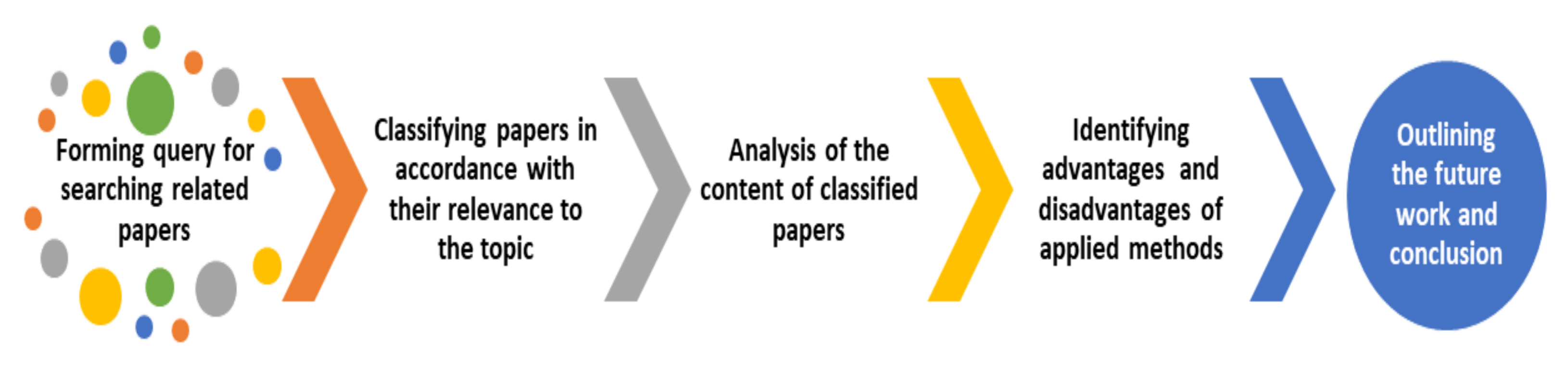
1.

The first step is a selection step that includes three important moments: time-frame, database, and keywords. As the ending point of the time-frame was selected as March 2022 when our investigations started. We expected to find results at the beginning of the time-frame. The origin of the paper was important when searching papers; thus, papers for our survey were selected from reliable Web of Science (https://clarivate.com/webofsciencegroup/solutions/web-of-science/ (accessed on 10 January 2022)) and Scopus (https://www.scopus.com/ (accessed on 15 January 2022)) databases. In order to properly conduct a search, Boolean operators were used alongside with topic-related terms and phrases.For searching, the following keywords were used: “poverty and AI”, “poverty” AND “AI”, “poverty and machine learning”, “poverty” AND “machine learning”, “poverty and deep learning”, “poverty” AND “deep learning”. In this stage, overall, we collected forty-three papers.

2.

The second step is a classification. All found papers were classified according to the following exclusion criteria: (1) papers theoretically describing the relationship between poverty and AI were excluded; (2) papers theoretically analyzing the impact of AI on poverty were excluded; (3) papers illustrating examples of AI applications in various spheres were excluded; (4) conference proceedings were excluded. The reason of these exclusion criteria is that the aim of our survey is to analyze the real applications of AI methods in poverty prediction. After reading abstracts and full-length papers, twenty-two papers were selected for our survey. Among these twenty-two papers, the remaining steps were performed. This classification step provided us with the beginning of the time-frame of our survey. It was revealed that the first paper on AI applications in poverty prediction was published in 2016; thus, this year was chosen as the initial benchmark of the time-frame of our conducted survey.

3.

In the third step, the content of collected papers was analyzed.

4.

At the last stage, the outcomes were discussed and future orients were provided.

In order to identify the tendency of publications on poverty prediction applying AI tools over the chosen time period, selected papers were divided according to the year of publication, and the outcome is illustrated in Figure 2. Overall, it can be seen that from 2016 to 2020, only a couple of papers were dedicated to AI applications in poverty prediction, and the boom happened in 2021 when seven papers were published in this sphere. This implies that researchers have become more interested in using AI tools for predicting poverty.

Figure 3 provides more detailed information on publications across the years, in which publications were categorized into two types in accordance with the applied approach to poverty measurement. Thus, above the line, papers where monetary approaches to poverty were considered are listed, whereas the papers shown below the line belong to a non-monetary poverty approach. In this figure, it can be seen that the distribution of poverty approaches among papers was equal. Yet, an interesting tendency can be observed when the initial analysis was conducted using the monetary approach to poverty, but as time passed, the non-monetary approach prevailed in poverty prediction via AI applications.

The above-mentioned graphs illustrate that there is currently a big demand in AI applications in poverty prediction, and it is time to publish comprehensive surveys on this topic to consolidate previously accomplished work for further research studies.

4. AI Tools in Poverty Prediction

This section is aimed at reviewing different applications of AI tools in predicting poverty. In each sub-section, a separate paper is analyzed with the description of used data, applied AI methods, and obtained results in order to find answers to our research question set in Section 1.

4.1. Combining Satellite Imagery and Machine Learning to Predict Poverty (CSIMLPP)

This work is a revolutionary study in predicting poverty from high-resolution satellite imagery [14]. As poverty measurements, consumption expenditure and asset wealth were chosen. Analyses were conducted using satellite data, and the Living Standards Measurement Study surveys five countries: Nigeria, Tanzania, Uganda, Malawi, and Rwanda. To measure household expenditures, authors used Living Standards Measurement Study (LSMS) surveys, whereas for wealth measurement, they used an asset index drawn from the Demographic and Health Surveys (DHS). Both these indicators were outcomes of the model.

Authors applied the CNN model, which consisted of three stages. Firstly, the model was pretrained on image classification data set (ImageNet). Next, CNN was trained to predict the nighttime light intensities corresponding to input daytime satellite imagery. Finally, cluster-level expenditures or assets were estimated. To extract features for the CNN model, convolutional filters and features corresponding to urban areas, nonurban areas, water, and roads were applied.

As an assessment of the model, the coefficient of determination ($R^2$) was applied. From the results, the predictive power for assets (55% to 75%) was higher than for household consumption (37% to 55%).

The authors compared their own model with a model where nightlights were the only input, and their model outperformed the latter for all countries.

They also revealed that their model worked better than the approach of using data from past surveys to predict outcomes in more recent surveys. In addition, they applied their model trained for one country in another country. As expected, in-country trained models performed better than out-of-country models, but the accuracy of out-of-country models was close to the in-country ones.

In conclusion, it should be noted that this study inspired many researchers illustrating the possibility of using daytime satellite imagery in poverty prediction.

4.2. Remote Sensing-Based Measurement of Living Environment Deprivation: Improving Classical Approaches with Machine Learning (RSBMLED)

This paper contributes to poverty measurement in urban areas by using high spatial resolution imagery data [15]. As poverty measurement Living Environment Deprivation (LED) was applied. The LED index is a part of the English Indices of Deprivation, which measures the quality of the local environment in terms of the quality of housing and the quality of the surrounding environment, and it consists of four indicators: housing in poor conditions, houses without central heating, outdoor air quality, and road traffic accidents [33].

An analysis was conducted for Liverpool (UK), where four sets of variables were extracted from a very high spatial resolution (VHR) image downloaded from Google Earth: a set of land cover features, a set of spectral features, a set of texture features, and a set of structure features. Land cover features illustrate different types of land cover: soil, vegetation, orange impervious surfaces (clay tile roofs and similar), gray impervious surfaces (asphalt and industrial roofing), water, and shadow. Spectral features represent the summary statistics (mean and standard deviation) of pixel values inside objects [34]. Texture features identify the spatial distribution of intensity values in the image, thus conveying information on uniformity and contrast [34]. The randomness of the distribution of the spatial arrangement of elements inside the polygons is characterized by structure features [34,35,36].

The authors used Google Earth images, combined them as a mosaic into geographic coordinates, and then projected this mosaic onto the same coordinate system of the spatial database of deprivation indices of Liverpool to obtain a georeferenced image with a pixel size of 70 cm. They used it as an input to calculate image-derived features for the same spatial units for which the LED index was reported.

One of the contribution of the paper is to create a model for estimating LED index, which was represented by formula $LED=f(LC;SP;TX;ST)$, where $f\left(\right)$ is a function of land cover (LC), spectral (SP), texture (TX), and structure (ST) data combination from each area and produces a prediction of its LED index. As input variables, the authors used sub-variables of these four sets of features: eight from a set of land cover features, six from a set of spectral features, eleven from a set of texture features, and ten variables from a set of structural features.

In the paper, the performance of two econometric models (Ordinary Least Squares Regression (OLS) and a Spatial Lag model (SL) based on the generalized method of moments) was compared with the performance of two machine learning methods: Gradient Boost Regressor (GBR) and random forest (RF). A hundred trees were grown for each RF and GBR model.

In model evaluation, the coefficient of determination ($R^2$) was applied. In evaluating models, the authors used two approaches: naïve ($R^2$) and honest (based on cross-validation [37]). In both naïve and honest approaches, machine learning methods were better, and RF was the best model. In the naïve approach, $R^2$ was 0.94 for RF and 0.83 for GBR models, whereas for OLS, this indicator was 0.34, and for SL it was 0.43. However, after implementing the honest approach, when authors conducted cross-validation (repeating the split-train-test procedure 250 times in each iteration), the $R^2$ for machine learning methods decreased dramatically from 0.94 to 0.54 for RF and from 0.83 to 0.5 for GBR. Yet, in the OLS model, the decrease comprised only 0.04 from 0.34 to 0.3.

Another contribution of the paper is in feature selection. Authors from all models concluded that the percentage of vegetation and the percentage of water had high predictive performance. Yet, it was claimed that the application of similar variables in other cities might result in different results with respect to the significance of variables; thus, the peculiarity of the city should be taken into account.

Overall, it can be said that AI tools performed better in comparison to econometric models.

4.3. Monetary and Non-Monetary Poverty in Urban Slums in Accra: Combining Geospatial Data and Machine Learning to Study Urban Poverty (CGDMLUP)

The paper proposes a methodology of slums identification and poverty rate prediction in urban areas by applying a combination of different data and machine learning tools [27]. The poverty rate at the neighborhood level was calculated using the small-area poverty estimation methodology [38].

The analysis was conducted for Accra city (Ghana) using three data types: household survey data, population census data, and geospatial data. As an imagery dataset an image mosaic of Quickbird-2 multispectral (Blue, Green, Red, and Near-Infrared) of the AMA (Accra Metropolitan Assembly) with a spatial resolution of 2.44 m was used. From this imagery, seven spatial and spectral features, representing the variability within the Enumeration Areas [39], were calculated for analyses. These features are the following: Line Support Regions (LSR), Histogram of Oriented Gradients (HOG), Linear Binary Pattern Moments (LBPM), PanTex, Fourier Transform (FT), the normalized difference vegetation index (NDVI), and the mean of the four original bands (Blue, Green, Red, and Near Infrared).

After data collection, the work was performed in three stages. Initially, the slum index was constructed by applying the random forest method, and the output was compared with official slums defined by UN-Habitat [40]. For this analysis, the same variables as in the UN-Habitat were used as input variables, adding population density and elevation explanatory variables. Elevation data were estimated by applying a Digital Elevation Model (DEM). Sub-samples of 50 % data were randomly selected 100 times from the total sample to calculate a slum score. Next, the slum index map was created. Furthermore, the model conducted feature selection, and the results showed that variables representing slum index significantly include elevation, population density, and the number of people per house.

At the second stage, the poverty rate at the neighborhood level was estimated. To estimate the poverty rate, population density and geospatial variables were used with the data of the 2010 Population and Housing Census and Ghana Living Standards Survey Round Six (GLSS 6). Overall, the variables represented four levels of the investigating area: household level, enumeration areas level, neighborhood level, and geospatial level. During model selection, a two-step procedure was conducted. Firstly, feature selection was conducted using a LASSO estimator with Bayesian shrinkage, according to which 15 variables were selected. Next, relying on the stepwise procedure, the final model was selected, where the selection criteria included the p-value. In addition, a poverty map was also created.

At the last stage, correlation and regression analyses between the slum index and poverty rate were conducted. Three different regressions were conducted, where the dependent variable was the poverty rate at the neighborhood level, and independent variables were household-head characteristics. The difference between the regressions is that the first regression used a slum index generated by random forest as an independent variable, whereas official slum data (slum areas) were used as an independent variable in the second regression. In the last regression, elevation was included as an independent variable to identify the concentration of poor people in low elevated areas.

From the results, it was revealed that a high level of women fertility, high monetary poverty, and poor school attendance were strongly associated with living in the slums of Accra. Furthermore, more poor people were concentrated in the lower-elevation areas, which could be explained by the fact that these areas were flood-prone. Other important variables explaining long-term poverty were ethnicity, religion, and region. Representatives of ethnic majorities tended to work in the manufacturing sector, whilst ethnic minorities and new migrants in poorer slum communities were employed in the wholesale sector. Generally, the outcomes illustrate various economic opportunities among slum communities.

4.4. Is Random Forest a Superior Methodology for Predicting Poverty? An Empirical Assessment (IRFSMPP)

The contribution of the paper that it proposes random forest algorithm applications for selecting model and predicting poverty status [13]. Poverty was defined as monetary poverty based on consumption expenditure aggregates. In poverty measurement, poverty proxies [41] were applied.

The household data of six countries (Albania, Ethiopia, Malawi, Rwanda, Tanzania, and Uganda) were used to conduct analysis, which included the following sections: demographics, education, food consumption, nonfood consumption, housing quality, ownership of durable goods, employment, and location.

In the paper, the traditional econometric model—Multiple Imputation (MI) [39]—was compared with a machine learning method—random forest (RF)—to identify which model could predict better. In constructing the RF model, standard settings were used. Five hundred trees were grown with a minimum of four observations in each leaf. Moreover, in the paper, steps involved in conducting the RF model were described precisely. Overall, in the paper, six models were created: MI with Stepwise variable selection, MI with LASSO variable selection, RF using Entropy loss function, RF using Gini impurity loss function, MI with 25 variables based on importance score from RF, and RF with 25 variables based on an importance score from RF. Models were assessed by applying the mean square error (MSE) between predicted and measured poverty rates.

The analysis process of the research consisted of two parts. Firstly, the data for one year were used. It was divided randomly into two parts, and half of the data were used for model generation, which was then tested in the second half of the data. Next, the same work was conducted, however, using the data for two years, where the first year was used for model creation and the second year served to assess the prediction capacity of the model.

It was revealed that the accuracy level of poverty prediction was higher when using RF. The poverty was calculated in three levels (urban, rural, and national), and results indicated that in urban and rural levels, the RF worked better rather than in the national one. When creating a model for one year, in urban and rural levels, RF had significantly higher accuracy in four out of six countries.

Yet, when making predictions for two years, all models were not accurate enough, and only about half of the models could predict poverty accurately. It was revealed that a consequence of the potential aging of the sample is an additional inaccuracy. Large variations in predictions for different models indicated that some models were incapable of taking price and economic changes into account.

In feature selection, Stepwise and LASSO methods were applied [21], and their outputs were compared with RF results, which also had an option of using importance scores for each variable. So, Stepwise and LASSO methods on average selected 81 and 132 variables, respectively, for six countries, whereas according to RF, 25 variables had the highest importance score. Prediction models were constructed based on variables, selected by RF. When the MI prediction model was constructed by relying on these 25 variables selected by RF, its accuracy improved in four out of six countries. The average accuracy for all models was also better with 25 variables.

4.5. Multidimensional Paths to Regional Poverty: A Fuzzy-Set Qualitative Comparative Analysis of Colombian Departments (FSQCACD)

The objective of the paper is to evaluate conditions that affect the capability deprivation of twenty-four Colombian regions [42]. In order to measure capability deprivation, two indicators were applied: monetary poverty (MP) and life expectancy (LE). Conditions impacting capability deprivation include economic (trade openness and GDP per capita), institutional (internal displacement and transparency), and social conditions (education coverage).

To achieve their aim, authors applied a Fuzzy-set qualitative comparative analysis (fsQCA). The strength of this method is that it can be applied even to small-sized samples, and the consolidated effect of a set of conditions can be assessed. The fuzzy sets in the paper were designed using five conditions and two outcomes (MP and LE). Boolean comparison of cases was conducted in the paper in terms of the absence or presence of certain conditions. Yet, the partial membership to a fuzzy set could occur which demanded the calibration process. In order to define full absence and full presence, the 10th and 90th percentiles were used as cutoffs, whereas the point of maximum ambiguity was determined using the median.

It was revealed that although there were attributes impacting on outcomes, none of them reached the 0.9 cutoff, meaning that no attribute played a determinant role in the presence of MP and LE. The most impactful attribute on MP was GDP per capita, whilst on LE, it was displacement. In the sufficient condition analysis, two methods were investigated: which configurations led to the presence of capability deprivation and which configurations led to the absence of capability deprivation. The authors illustrated four pathways to high regional MP and two pathways to low regional MP, whereas for LE, they represented three pathways for high LE and three pathways for low LE. This technique empowered the classification of regions with respect to pathways.

Finally, a general model was developed, which included all possible configurations that could explicate high MP rates in regions. The model’s score of consistency comprised 0.9, implying its interpretation’s robustness. It should be noted that there was no universal pattern that could be applied to all high MP regions, yet economic and institutional attributes were important in defining MP.

It can be concluded that the application of fuzzy set provides a deeper analysis of poverty by offering different combinations of attributes, which may lead to increasing or decreasing poverty rates. From this study, it can be seen that even for different regions of one country, there is no universal pattern explaining poverty.

4.6. Retooling Poverty Targeting Using Out-of-Sample Validation and Machine Learning (RPTOVML)

The aim of this paper is to improve the proxy means testing (PMT) tool to identify poor people for social program targeting [16]. The main problem in targeting is the existence of leakage and undercoverage rate, and authors aimed at improving poor people identification from out-of-sample data. In addition, the goal of PMT is not only to categorize poor people but also to find significant variables characterizing poverty that would perform well in any data and country.

LSMS data and household surveys of Bolivia (2005 year), Malaawi (2004–2005 years), and East Timor (2001 year) were used for analysis. The sample data had different sizes among these countries; in particular, Malaawi had the largest number of observations (11,280), whereas this figure comprised 4086 for Bolivia and it was 1800 for East Timor. Yet, for these countries, the variables were not similar: household characteristics had some discrepancies.

In the paper, the USAID poverty assessment tool [43] was applied, and two methods were compared, econometric (cross-validation) and machine learning (stochastic ensemble methods [44]), to identify which of them would be more accurate. Authors used PMT tools developed by the University of Maryland Institutional Reform and Informal Sector (IRIS) Center to demonstrate methods for USAID poverty assessment. In evaluating PAT tools, the following metrics were used: total accuracy, poverty accuracy, undercoverage rate, leakage rate, and balanced poverty accuracy. Balanced poverty accuracy penalizes the poverty accuracy rate with the extent to which the leakage and undercoverage rates exceed one another.

In stochastic ensemble methods of machine learning, the following algorithms were applied: regression tree, random forest, and quantile regression forest. It was emphasized that the quantile approach is particularly useful for investigating poverty; in other methods, the conditional mean is used, yet poor people are concentrated far from this mean. Five hundred trees were grown for each algorithm.

Authors compared results from replicating IRIS models, cross-validation, and stochastic ensemble methods for three countries according to the total accuracy, poverty accuracy, undercoverage, leakage, and balanced poverty-accuracy indicators. It was revealed that cross-validation and stochastic ensemble approaches were prompt in classifying non-poor as poor. In particular, authors found that the application of cross-validation and stochastic ensemble methods to the problem of developing a poverty-targeting tool could produce a gain in poverty accuracy, a reduction in undercoverage rates, and an overall improvement in balanced poverty accuracy criterion in comparison to traditional methods.

4.7. Machine Learning Approach for Bottom 40 Percent Households (B40) Poverty Classification (MLB40)

The aim of this paper is to select the best model for the precise identification of the bottom 40 percent of households (B40) in Malaysia [17]. The national poverty line based on income served for poverty measurements.

National Poverty Data Bank, called ‘eKasih’ was used as a dataset [45]. From this dataset, the authors used information on 99,546 households of three states, namely Johor, Pahang, and Terengganu. Overall, 15 variables were used: state, area, strata (urban/rural), ethnic, marital status, age, gender, job, education, type of ownership, household number, total income, income per capita, date of record, and poor status.

Authors applied Naive Bayes [46], Decision Tree (J48 classifier, based on the C4.5 algorithm) [47], and k-Nearest Neighbors [48] algorithms for their purpose. The classification performance of models was analyzed using Classification Accuracy and Kappa Statistic [49].

Before creating models, data pre-processing tasks were conducted with respect to the raw dataset to ensure the quality of the training data. These data pre-processing tasks include cleaning [48], feature engineering, normalisation [50], feature selection [51] (Correlation Attribute, Information Gain Attribute, and Symmetrical Uncertainty Attribute), and sampling methods using SMOTE [52].

The first step of the pre-processing task is data cleaning, when missed variables were replaced. Next, feature engineering was conducted. A new variable, such as Median Monthly Income, was created by dividing the total income to 12. Then, a pre-labelled class for B40 was manually generated, relying on thresholds for each state. Here, two classes were created: B40 and not-B40. The third step was conducting a normalisation procedure for certain variables, making them fall between 0 and 1. Fourthly, a feature selection procedure was conducted by applying three ranking methods: Correlation Attribute, Information Gain Attribute, and Symmetrical Uncertainty Attributes. According to all three ranking methods, the top-eight variables are: state, area, ethnic, household number, total income, average monthly income, income per capita, and date of record. As the final stage, the selection of the sampling method was conducted. The problem with dataset was that there was an imbalance between B40 (majority—94,495 households) and not-B40 (minority—5051 households), with a ratio of 5:95. This could lead to biases towards the majority class. In order to overcome this problem, the Synthetic Minority Oversampling Technique (SMOTE) was applied, when synthetic minority examples were generated to oversample the minority class. SMOTE is then applied to the dataset at 400% over sampling degrees with nearest neighborhoods numbering at five, increasing the minority class from 5051 to 25,255 instances. So, after sampling, instead of 99,546 instances, there were 119,750 instances, and the imbalance ratio comprised 21:79.

After pre-processing procedures, each classifier was then optimized using a different tuning parameter with 10-Fold Cross Validation for achieving the optimal values before the performance of the three classifiers were compared with each other. For Naïve Bayes, discretization was used as a tuning parameter. For the decision tree, minimum numbers of objects [53] and confidence factor [47] (from 0.1 to 1.0 by an increment of 0.2) were used as tuning parameters. For the k-Nearest Neighbor algorithm, the k-value was investigated from 1 to 10 to identify the optimal value for the training samples [54]. In addition, four distance functions were examined in the tuning process: Euclidean distance, Chebyshev distance, Manhattan distance, and Minkowski distance [55].

Models were created twice: initially, 16 variables are used and then 8 top significant variables are used. Interestingly, the outcome was more accurate in the latter case (the average accuracy increased from 93.35 % to 95.76 %).

Moreover, authors represented results with models before tuning and after tuning parameters. For Naïve Bayes, after discretization, the accuracy level increased from 91.52 % to 97.27 %. For the decision tree, the optimal value of the confidence factor was 0.4 (accuracy level was the highest—99.27). An increase in the minimum number of objects decreased the accuracy; thus, the optimal value for the minimum number of objects parameter was chosen as 2. For the k-Nearest Neighbors algorithm, a k-value was chosen as 1, and the Manhattan distance was used as a distance function for the best and most accurate performance. When comparing models, according to both Classification Accuracy and Kappa Statistic, the decision tree performed with the highest accuracy (99.27% and 0.98), whereas the least accurate model was the k-Nearest Neighbor (96.80% and 0.90).

4.8. A Comparison of Machine Learning Approaches for Identifying High-Poverty Counties: Robust Features of DMSP/OLS Night-Time Light Imagery (NTLIML)

The aim of this study is to illustrate that with the help of only DMSP/OLS, nighttime light-imagery machine learning can identify robust classification features as well as high-poverty counties [18]. For poverty identification, 15 features were extracted from nighttime light imagery and trained with 96 high-poverty counties and 96 non-poverty counties in 2010. These 15 features can be considered from three aspects: central tendency (four features), degree of dispersion (three features), distribution features (seven features), and spatial feature (one feature). In order to decrease discrepancies, a modified invariant region (MIR) method was applied to desaturate the image [56].

In the paper, 2554 counties of 31 Chinese provinces were studied. To reach the aim, seven models were applied: Gaussian process with radial basis function kernel (GPRBFK) [57], stochastic gradient boosting (SGB) [58], partial least squares regression for generalized linear models (PLSRGLMs) [59], random forest (RF) [60], rotation forest (RoF) [61], support vector machine (SVM) [62], and neural network with feature extraction (NNFE) [63].

Class probabilities (0 1) were acquired during classification; then, a threshold was selected as the cut-off between the two classes (when the probability was closer to 1, it implied a higher probability of the county being poor) [64]. Counties were considered as high in poverty when the probability of their poverty was larger than 0.6.

Five feature importance measures were adopted to evaluate feature importance levels for the seven machine learning approaches. In RF, mean decrease Gini and permutation accuracy importance were applied for feature importance measurements; in RoF, the sum of the decrease in impurity was used; in SGB, the sum of squared error was used, whereas the remaining models used a receiver operating characteristic curve.

Three types of accuracy were used to measure the classification’s accuracy: user’s accuracy, producer’s accuracy, and overall accuracy. The user’s accuracy and producer’s accuracy both exceeded 63%, which indicates that all machine learning approaches provide accurate identification results, which is also supported by the fact that all overall accuracies were greater than 82%.

The classification performance of each machine learning approach was different. In total accuracy, GPRBFK had the highest accuracy level (84.67%), whereas PLSRGLM had the lowest accuracy level (82.85%).

Overall, from all different applied methods, it was revealed that statistical features that defined poverty more included F1 (variance of all pixels within the county boundary), F8 (total value of all pixels within the county boundary), F6 (standard deviation of all pixels within the county boundary), F5 (variance of all pixels within the county boundary), and F10 (number of pixels greater than zero within the county boundary). This result represents that the different aspects of nighttime light features reveal both the development and the relative poverty in each region.

It should be noted that F15 (Local autocorrelation Moran’s I of the counties) made a particularly important contribution to the classification; this variable was the first or second most important feature for some of the approaches used in this paper and indicated the importance of spatial features in the poverty identification task. Moreover, the importance of this spatial feature illustrates that its contribution to the classification result is almost irreplaceable.

Finally, Pearson’s correlation analysis was conducted to analyze effects of the importance of each feature on the classification’s results. According to authors, at least nine features should be used in models to ensure the overall accuracy.

4.9. Estimation of Poverty Using Random Forest Regression with Multi-Source Data: A Case Study in Bangladesh (MSDRFR)

The aim of the paper is to construct a random forest regression (RFR) model for poverty estimation at 10 km resolution from different datasets [65]. The analysis was conducted in Bangladesh, and the created model was also applied in Nepal. As a poverty measurement, the household wealth index (WI) was applied.

Data for WI construction was derived from the DHS dataset for Bangladesh, which consisted of 598 household clusters. Each cluster on average contained 28.8 households, whilst the median number of households inside clusters constituted 29. NTL data for 2015 was obtained from The VIIRS Cloud Mask–Outlier Removed (vcm–orm) annual composite NPP-VIIRS DNB dataset. To extract the landscape’s texture and structure features, Google satellite images for the period of 2015–2017 were used. To compute the region’s accessibility, data on primary and secondary roads were excavated from the OSM dataset. Land cover features were extracted for 2015 from land cover maps at a 300 m resolution. The Gaussian mixture model, CNN model named VGG-F [66], and principal component analysis were conducted for features extraction. In total, 36 variables representing four dimensions of poverty estimation were extracted: socioeconomic, accessibility, land cover, and structure and texture. After extraction, these features were used as independent variables, whereas WI served as a dependent variable.

In the analysis, RFR was applied. Before implementing RFR, standardization procedures were conducted, followed by the method of backward elimination [67]. In model creation, a ten-fold cross validation approach was used. The performance of the model was assessed using $R^2$ between the actual and estimated WI, whereas the explanatory power of features was measured by the Gini importance metric.

According to results of feature selection, 14 variables out of 36 were selected. It should be noted that the highest weight among variables were obtained by variables representing accessibility (42.2%). The mean NTL was the second variable by importance level (32.6%).

Using the 14 selected variables, an RFR model was created. $R^2$ of the proposed model comprised 70%. In order to check the validity of the model, the same analysis was conducted for Nepal with Nepal data. In case of Nepal, $R^2$ constituted 0.61%.

Next, a 10*10 poverty map based on WI for Bangladesh was created using RFR, which was compared with the Head Count Rate (HCR) map derived from 2015 survey data [68]. The Jenks natural breaks method [69] was applied to classify both maps into five grades. The patterns of these maps were almost similar. Moreover, Pearson’s correlation coefficient was calculated between WI and log-transformed HCR. It admitted the existence of a negative relationship between these indexes (0.6).

One of the limitations of the model was that it tended to overestimate low WI values and underestimate high WI values because the output of RF was the average result of all trees. Another limitation was the existence of a multicollinearity issue between independent variables.

It can be concluded that RFR has a good predictive power in estimating poverty by integrating different datasets. In the case of Bangladesh, it was revealed that accessibility was the most impactful factor in poverty explanation.

4.10. Ensemble Learning for Multidimensional Poverty Classification (ELMPC)

The aim of the paper is to conduct poverty classification by applying the random forest (RF) method on a Malaysian dataset, eKasih, for 2017 [70]. For poverty measurements, the Multidimensional Poverty Index created by the Malaysian Government was applied. This index contained four dimensions (education, health, living standards, and income) and eleven indicators.

Overall, 196,650 observations and 24 variables were used in the analysis. These variables express different dimensions, including household information (two variables), income (two variables), health information (three variables), household location (nine variables), and household demographic (eight variables). Yet, based on the literature review, only 15 variables were selected out of 24. Before applying machine learning methods, data management was conducted by the Cross Industry Standard Process for Data Mining (CRISP-DM) Methodology applications. This methodology has six stages: Business Understanding, Data Understanding, Data Preparation, Model Development, Model Evaluation, and Deployment [71].

Two machine learning methods, RF and decision tree (J48), were applied to find the most accurate method. In RF, the authors grew 100 trees. For training purposes, Poverty Status variables were selected as a class label. It was revealed that more trees led to error rate reductions. In J48, eight rules were used that served to classify poor and hardcore poor people. In order to assess model accuracy, a confusion matrix [72] was created. Moreover, an indicator such as Receiver Operating Characteristic (ROC) was applied to measure the sensitivity of the prediction [73]. The accuracy level of RF comprised 99 %, whereas the accuracy level of J48 was 98 %. In ROC, the area under the curve (AUC) value is taken into consideration, where the higher AUC means a better model. The AUC value of RF and J48 constituted 0.9999 and 0.9975, respectively.

In order to find the most impactful variables among 15 variables, the Mean Decrease Gini (MDG) indicator in RF and the Information Gain indicator in J48 were applied. RF picked out five variables as important: per capita income, states, ethnic, strata, and religion. For J48, only three variables were enough: per capita income, strata, and state.

The results of RF variable ranking were compared with the varImp function in R language for the linear model. In ranking, the median for mean rank was calculated (0.065), which served as a line for variables being considered as important. The higher the mean rank of the variable, the higher its importance level in poverty identification. In total, seven variables were selected as the most important variables in poverty classification: per capita income, state, ethnic, strata, religion, occupation, and education.

Finally, RF and J48 models were created using the above-mentioned seven variables. The results represented showed that the accuracy level of models remained unchanged in comparison with previous models, yet processing times improved (from 31.64s to 14.97s in RF and from 3.34s to 1.39s in J48).

4.11. A Social Engineering Model for Poverty Alleviation (SEMPA)

The aim of the paper is to determine a poverty line based on agent-based stochastic model of market exchange which includes labor, commodity, and asset market outcomes [74]. In order to calculate the poverty line, machine learning tools were applied. As a poverty measurement, the consumption of three types of products was chosen: cereals, other food, and non-food.

According to authors, modern approaches to poverty have two main weaknesses. The first one is that consumption deprivation (CD) [75] or poverty is not linked with the overall economic system that causes this phenomenon. The second pitfall is the absence of prediction methods of upcoming poverty rates as a function of controllable economic variables.

For analysis, the NSS income data of 23 years for India were used [76], and they were correlated with expenses on cereals, other-food, and non-food products. In order to obtain the multivariate version of Engel plot’s [77], these three types of expenses were combined into a single (non-dimensional) function using independent multivariate models—Neuroscale [78], Locally Linear Embedding (LLE) [79], Isomap [80], Curvilinear Component Analysis (CCA) [81], and Principal Component Analysis (PCA) [82]. Authors also tried to find weights from a dimension reduction algorithm, whereas measurement weights are arbitrary in the traditional multidimensional poverty index (MPI). It was suggested that scalar weights in reality are the market prices. According to the PCA method, the weights for cereal, other-food, and non-food dimensions comprised 0.1694, 0.4336, and 0.8851, respectively. Thus, it served as a basis for the agent-based model (ABM) to represent the mechanism of competitive markets by establishing the equilibrium of prices and quantities, after which the Langevin and Fokker–Planck model was created [75,83,84,85].

Results indicate that even when using dimension reduction tools, information can be preserved. The highest level of preservation was with Neuroscale and Isomap, and lower preservation was observed when used with others. Next, in order to identify the level of the relative importance of dimensions, NeuroScale mapping was applied. Interestingly, as weights were not constant, they varied with income. Thus, when the expenditure level was low, the weight of other-food was the highest, whereas with an increase in expenditure levels, the weight of non-food items also started increasing. In order to prove the model, it was trained on the Indian dataset for 30 years (1959–1991) and also tried on the USA dataset. The outcome of algorithms was assessed using an indicator of standard deviation from real data.

Results from applying the model from both countries showed that the total poverty index estimated from multivariate dimensions had lower values in comparison with the poverty index derived from only cereal consumption. According to the authors, poverty measurements should have multivariate constructions, which means that all modes of income and expenditure need to be considered for proper weighting. Furthermore, machine learning performs better in economic prediction when it is combined with statistical mechanics-based models. This is the reason of the under performance of machine learning, as only machine learning without statistical integration was used for poverty modelling in many studies.

4.12. Measuring Urban Poverty Using Multi-Source Data and a Random Forest Algorithm: A Case Study in Guangzhou (MUPMDRF)

The aim of the paper is to develop a new approach in urban poverty measurement using multi-source big data [86]. This new measurement is called the Multi-source Data Poverty Index (MDPI), and it was created by applying RF. The idea of creating this index is that the built environment is also important in reflecting poverty along with census data.

Different types of data were applied for creating RF model: points of interest (POI) [87], nighttime light image [88], Landsat 8 image [89], housing rent data [90], and census data. This model was created for Guangzhou, China.

The analysis part had two stages. Initially, indicators of material, economic, and living conditions were generated from different datasets. These indicators were next categorized into five groups: facility and service provision, land-cover composition (vegetation, building, and water body), building texture, activity intensity, and housing cost. The RF model was created using generated indicators such as input data, which was trained using the General Deprivation Index GDI [91].

After creating MDPI for Guangzhou, the spatial distribution of each indicator was analyzed. For this purpose, maps were created by applying the Jenks Natural Breaks Classification Method [92]. Next, the relationship between each indicator and the GDI was assessed using Pearson’s correlation coefficient. It was revealed that all indicators had a statistically significant relationship with GDI. Moreover, the correlation was conducted between GDI and MDPI, and it comprised 0.954 with a p-value of 0.000.

In RF, ten-fold cross-validation was applied to estimate MDPI for 1735 communities. The model was assessed by applying the coefficient of Spearman’s rank correlation as well as the median relative error between the GDI and MDPI. The correlation between GDI and MDPI comprised 0.954 with a p-value of 0.000, whereas the median relative error constituted 18.3%. In addition, to assess the consistency level of GDI and MDPI, Z-scoring was applied [93]. According to the Z-score result, there is a linear relationship between GDI and MDPI with the consistent judgment rate of 89.9 %.

In order to identify the spatial autocorrelation’s degree of MDPI, the global Moran’s I value was generated [94,95], which comprised 0.518 with a p-value of 0.01. This result represented the existence of a significant level of spatial autocorrelation of MDPI. Furthermore, to analyze in depth the spatial autocorrelation of the intra-regional level, Local Indicators of Spatial Association (LISA) were performed.

Results of the model revealed that the classification of communities possessing similar characteristics can be classified into a high level with MDPI. The difference between GDI and MDPI is that GDI performed better in the inner-city area, which had a long urbanization period, whereas MDPI was more effective with the outer suburban area, which had been experiencing urbanization changes.

4.13. Estimating City-Level Poverty Rate Based on e-Commerce Data with Machine Learning (ECDML)

This paper represents an interesting approach in poverty measurement [22]. E-commerce data were used to estimate poverty rates at the city-level. For this purpose, two machine learning methods were applied: deep neural network (DNN) [96] and support vector regression (SVR) [97]. The estimated poverty rate was compared with the poverty rate calculated by BPS—Statistics Indonesia [98].

The e-commerce data were taken from the olx (https://www.olx.com/ (accessed on 16 February 2022)) platform of advertisements for goods in 2016. In the paper, in total, 18,881,913 advertisements were used, which were posted in 118 cities/districts of Java Island (Indonesia). Eight types of goods were analyzed in the model: cars, motorbikes, houses for sale, houses for rent, apartments for sale, apartments for rent, land for sale, and land for rent. For each good, information about sale prices, number of sold goods, number of viewers, and number of buyers was collected per city, and their sum, average, and standard deviation were calculated individually. Overall, in the analysis, 96 features were extracted from the e-commerce platform and normalized between 0 and 1.

The feature selection process was conducted by applying fast correlation-based filter (FCBF) [99]. The result of FCBF represented that the model could be created using only 29 features and not all 96 features. For robustness checking, for each machine learning algorithm, two feature sets were used with 96 features and with 29 features; thus, in total, four models were created. According to FCBF, out of eight goods, the largest number of selected features (five each) had motorbikes and cars, which implied that they were important goods in poverty estimations for Java Island.

After conducting all these pre-processing tasks, four machine learning models were created: SVR (with 96 features), FCBF-SVR (with 29 features), DNN (with 96 features), and FCBF-DNN (with 29 features). In creating SVR models, a radial basis function was applied for dealing with non-linear data. In DNN models, two hidden layers were used, as with one or three layers, the output of the prediction was insignificant. In the paper, the algorithm of DNN training was provided. The performance of the model was assessed using four indicators: root mean squared error (RMSE), R-squared ($R^2$), accuracy factor (Af), and bias factor (Bf) [100].

When comparing SVR and FCBF-SVR models, SVR had better performances with a lower RMSE (3.860 vs. 4.152), higher $R^2$ (0.430 vs. 0.361), and lower Af (1.152 vs. 1.169). The prediction was underestimated only in SVR (Bf = 0.967) in comparison with FCBF-SVR.

The performance of the DNN model was almost the same as the SVR model, and it had a higher $R^2$ (0.448), higher RMSE (3.945), and higher Af (1.155). Yet, after creating the FCBF-DNN model, the prediction performance improved with a lower RMSE (3.752), and this model was better than the SVR model. Thus, the FCBF-DNN model was applied for poverty prediction in Java island.

Overall, it was illustrated that e-commerce data can serve as a good complement to official poverty prediction procedure.

4.14. Poverty Mapping in the Dian-Gui Qian Contiguous Extremely Poor Area of Southwest China Based on Multi-Source Geospatial Data (PMMSGD)

The aim of the paper is to create a map of the integrated poverty index (IPI) for the Dian-Gui-Qian area (China) using remote sensing data and machine learning algorithms [101]. Traditional multiple linear regression (MLR) and seven machine learning methods were applied to choose the best IPI predictive model, which was used for poverty mapping purposes. As a poverty measurement, IPI was applied. IPI was created by integrating 13 social and economic variables that represent four dimensions (economic development, health, living conditions, and education) of poverty.

Social and economic variables were taken from official state publications, whereas different datasets were used to analyze spatial features: NPP/VIIRS NTL data, Finer Resolution Observation and Monitoring Global land cover (FROM-GLC) data, open street map (OSM) data, SRTM digital elevation model (DEM) data, natural disaster data, and accessibility to cities [102]. Overall, eight spatial data were extracted from the mentioned above datasets. Thus, the average nighttime light (NTL) was taken from NPP/VIIRS dataset, the altitude (H) and the flat area coverage (FAC) were derived from the SRTM/DEM data, traffic accessibility (TA) was provided by the city accessibility data, road density (RD) was computed from the OSM data, the impervious surface coverage (ISC) and cropland coverage (CC) were extracted from FROM-GLC data, and a composite risk index (RI) including multiple hazards was derived from the Global Risk Data Platform to collect natural disaster data. This index ranged from 1 (low) to 5 (extreme).

In the analysis process, for verification purposes of the performance of the model, ten-fold cross-validation was applied in which the entire dataset was randomly divided into ten parts, nine of which were used for training and one was used for testing process. This process was repeated 10 times. In the paper, MLR was applied together with the following seven machine learning models: bidirectional recurrent neural network (BRNN), generalized additive model (GAM), support vector machine (SVM), MARS, random forest (RF), XGBoost, and Cubist. In evaluating model performance, the mean absolute error (MAE) and coefficient of determination ($R^2$) were used. The model with the best accuracy was applied to estimate final IPI model.

Results illustrate that the best model was XGBoost with the MAE and $R^2$ equaling 0.0479 and 0.61, respectively, followed by GAM (MAE = 0.0498; $R^2$ = 0.59) and RF (MAE = 0.0527; $R^2$ = 0.57) models. The performance of MLR model had the lowest accuracy level (MAE—0.0767 and $R^2$—0.23). Thus, for the final model, XGBoost was applied.

Moreover, feature selection was conducted to overcome the overfitting problem. Five variables were selected (NL, TA, RI, RD, and FAC) to conduct the XGBoost model. Among these variables, NTL had the highest importance (38.51%) rate. When XGBoost was created with these five variables, its performance improved (MAE = 0.0454, $R^2$ = 0.68). After creating the final XGBoost model with five variables, the predicted IPI was compared with actual IPI values. According to the results, the predicted IPI values were almost similar to the actual ones. Only in wealthy areas was the IPI (IPI > 0.5) slightly underestimated. Next, a poverty map was created and compared with the actual IPI map. It was revealed that in most areas, the error comprised approximately 15%, and only in few areas were errors higher than 30%. This means that the IPI map created on remote data can effectively predict the poverty distribution.

From results, it can be concluded that remote data can be useful in poverty prediction. When compared linear regression and machine learning methods, the latter were more effective. Finally, it was revealed that models with fewer variables can serve to provide better prediction capacity.

4.15. Combining Night Time Lights in Prediction of Poverty Incidence at the County Level (CNTLPP)

The aim of the paper is to show that machine learning can be applied in identifying and predicting poverty at the county level [103]. In measuring poverty levels, a poverty incidence indicator was applied [104]. The Yunnan–Guangxi–Guizhou Rocky desertification (YGGRD) area (China) was taken as a focus area of the research study. In the paper, seven classification learning models (Decision Trees, Discriminant Analysis, Logistic Regression Classifiers, Naive Bayes Classifiers, SVM, Nearest Neighbour Classifiers, and Ensemble Classifiers) were applied to identify whether the county is poor, and five regression learning methods (Linear Regression Models, Regression Trees, SVM, Gaussian Process Regression Models, and Ensembles of Tress) were used to predict poverty incidence.

Nighttime data were extracted from DMSP/OLS (1992–2012 years) and NPP/VIIRS (2013–2018 years) datasets. To correct the difference between these datasets, the modified invariant region (MIR) method was applied [105]. Poverty incidence data were taken from official statistical sources. The poverty incidence for the period 1992–2018 was predicted in the study for the focus area by using specific NTL and poverty incidence variables of 88 counties in the Guizhou Province for 2012 and 2013 years as the training data set. The following five variables of remote-sensing data were used for analysis: the total value of the pixel digital number (DN) (Sum) corresponding to the NTL data, the average value of pixel DN (Mean), the range of pixel DN (Range), the variability of pixels in the county (variety) areas, and the standard deviation of pixel DN (Std) [18,106,107]. In the analysis, these features served as independent variables, and poverty incidence was a dependent variable.

Classification and regression models were assessed using different indicators. A receiver operating characteristic (ROC) curve and a confusion matrix (CM) were applied to evaluate classification models, whereas regression models were assessed using the root mean squared error (RMSE), mean absolute error (MAE), and the $R^2$ value of the predicted and actual values [18,108].

Among classification models, SVM had the highest accuracy level (76.5%), yet it was not so effective among regression models. Among regression models, according to all three parameters, The Regression Tree algorithm outperformed all models with an RMSE equal to 5.0143, MAE equal to 4.0415, and $R^2$ equal to 0.60 (which is almost twice as higher as in the other models). Thus, SVM was chosen to conduct the classification regression for 1992–2018, and the decision tree was selected for poverty incidence prediction for 1992–2018.

As the next step, to identify whether the created model can identify poverty-stricken areas, SVM was applied for the 2012 year, and its result was compared with actual official data. Thus, results indicated that the created model had the 82.35% of the correct rate for poverty-stricken counties. It was revealed that the model was inclined to identify non-poverty-stricken areas as poverty stricken areas. To create a model for poverty prediction for the 1992–2018 period, the regression tree model was applied. According to its result, poverty reduction in the region could be divided into three stages, when the last stage showed a significant reduction in poverty. Furthermore, to illustrate the spatial distribution of poverty incidence, spatial mapping and hot-spot analysis were conducted in the study for three years (1992, 2005, and 2018).

It can be concluded that different machine learning perform differently according to the purpose of their application, either with respect to classification or prediction. Results of the study indicate that NTL data can represent the poverty incidence effectively, and machine learning is a powerful tool for poverty analysis in the county level.

4.16. A Novel DBSCAN Clustering Algorithm via Edge Computing-Based Deep Neural Network Model for Targeted Poverty Alleviation Big Data (DBSCANECDNN)

The aim of the paper is a development of a new model called the DBSCAN Clustering Algorithm via Edge Computing-Based Deep Neural Network for poor households identification. This method can conduct identification via determining the poverty features of poor households [109].

The DBSCAN algorithm belongs to the family of clustering algorithms that are based on density. In clustering, the Eps neighborhood of each data object is calculated. The strength of this algorithm is its capacity for the automatic determination of class clusters’ number, finding the shape of class clusters, and its insensitivity to noise data.

The proposed model was compared with three other models: CDBSCAN [110], FSDBSCAN [111], and NARDBSCAN [112]. To assess the performance of all models, precision (PRE), F-measure, and normalized mutual information (NMI) indexes were applied, where the value of these indexes was between 0 and 1. The closer the index to 1, the better the performance.

In the paper, four experiments were conducted. The first three experiments were conducted using datasets of the machine learning repository [113] and by applying four algorithms. Results indicated that the DBSCAN algorithm outperformed all other methods by all parameters. In addition, it also had the highest accuracy rate (99.36%) as well as the highest speed in analysis (55.5 ms).

The fourth experiment was conducted using real poverty alleviation data, which originated from a prefecture-level city, including 11,423,500 from rural population, 196,700 from rural households, and 68,000 from poverty-stricken households. The original data included the data of an archived card, the data of an agricultural cloud project, the data of visits, and the data of education, health, and sanitation departments. By applying the clustering algorithm, feature classification was conducted, which identified eight clusters, where each cluster corresponded to a feature category.

According to results, the accuracy level was the highest in the proposed DBSCAN model (96.5%). Moreover, in the proposed method, the analysis process constituted only 1358 s, whereas in other models, the analysis time was calculated during several days from 2.5 days (NARDBSCAN) to 7 days (CDBSCAN).

It can be concluded that the DBSCAN Clustering Algorithm via Edge Computing-Based Deep Neural Network can be a useful tool in poverty identification with higher accuracy and quicker calculations.

4.17. Identifying Urban Poverty Using High-Resolution Satellite Imagery and Machine Learning Approaches: Implications for Housing Inequality (HRSIML)

The aim of the paper is to identify urban poverty at the community level using high-resolution satellite imagery and applying four machine learning algorithms (RF, Gaussian Process Regression (GPR), Support Vector Regression (SVR), and Neural Network (NN)) [114]. The study area was Jiangxia District and Huangpi District, Wuhan, China. The poverty incidence was used as a measurement of urban poverty.

Three datasets were used in the analysis: Google Earth imagery, land cover dataset and the boundary of administrative divisions, and population census and poor population statistics of neighborhood and village committees. Data were taken for 2016. Image features contained geometric, shape, and texture features, which included perimeter [115], line segment detector (LSD) [116], the gray-level co-occurrence matrix (GLCM) [117], local binary patterns (LBP) [118], Hough transform [119], and a histogram of oriented gradients (HoG) [120]. Overall, 25 variables were employed in model creation.

In the analysis, the dataset was divided into three parts, two parts of which were used for training and the third for validation. Four machine learning models were created and their performances were compared with each other. The model’s performance was assessed using the coefficient of determination ($R^2$). Moreover, for RF, the Mean Decrease Gini (MDG) and Permutation Accuracy Importance (PAI) indicators were used, whilst for the remaining models, the receiver operating characteristic curve (ROC) was used to select the most impactful features.

Results indicate that the SVR model had the best performance for both districts with $R^2$ equal to 0.53. The worst model for Jiangxia district was NN with an $R^2$ equal to 0.3492, whilst for Huangpi, it was GPR with an $R^2$ equal to 0.4231. Furthermore, the poverty mapping using the local indicator of spatial association (LISA) was conducted to identify committees of concentrated poverty and to see if the predicted poverty incidence from remote sensing using NN can recognize the same committees as the survey-based poverty incidence. It was revealed that the fitness of the model was good in the given areas without deviations toward low or high values.

When identifying important variables, models showed different important scores for variables. Yet, there were variables that were relatively important in urban poverty identification, namely F18 (Histogram skewness), F17 (Histogram kurtosis), F7 (GLCM entropy), F6 (GLCM uniformity), F9 (GLCM inverse difference moment), and F10 (GLCM covariance). These variables illustrate the importance of GLCM and HoG for describing the characteristics of built-up areas with different poverty levels.

Next, machine learning algorithms were applied by using different combinations of variables to identify the most significant variables. Different results obtained different combinations of variables and models. According to their results, models with five variables (F18, F17, F7, F6, and F9) were more accurate, with an $R^2$ ranging from 0.2903 to 0.5189.

It can be concluded that machine learning is effective in feature extraction from high-resolution satellite imagery and also useful in poverty identification and feature selection. It was revealed that four applied machine learning models showed different levels of accuracy with various combinations of features.

4.18. Multivariate Random Forest Prediction of Poverty and Malnutrition Prevalence (MRFPPMP)

The paper aims achieving two goals: (1) contemporaneous mapping poverty and malnutrition indicators and (2) nowcasting near future poverty levels based on current remote-sensing data and historical observations [121]. In order to reach these goals, machine learning methods were applied using remote-sensing data.

Data of eleven countries, namely Bangladesh, Ethiopia, Ghana, Guatemala, Honduras, Kenya, Mali, Nepal, Nigeria, Senegal, and Uganda, which are USAID Feed the Future priority countries, were used in the analysis. Indicators of poverty and malnutrition were used from the DHS or Advancing Research on Nutrition and Agriculture (ARENA) [122] aggregated DHS data or directly from the DHS [123]. Poverty and malnutrition estimation aggregates on the level of clusters or enumeration areas (EAs) were extracted from DHS and ARENA datasets. Asset poverty, healthy weight, child wasting, child stunting, and underweight women were used as dependent variables. As independent variables, six sets of covariates were used: physical geography covariates (travel time to the nearest city with a population of 500,000 or more persons [102], percent tree cover data [124], pasture coverage data [125], altitude measured as the pixel elevation in meters above/below sea level, slope, calculated by the IFPRI ARENA team as the degree gradient of steepness), food price data (food types, number of geographic markets, and whether the data reflect retail or wholesale prices) [126], solar-induced chlorophyll fluorescence (SIF) data [127], land surface temperature (LST) data [128], precipitation data [129], and conflict data (number of violent events and number of resulting casualties) [130].

In the analysis, independent RF (IRF) and multivariate RF (MRF) [131,132,133] were applied for poverty prediction and malnutrition prevalence. The difference between both methods is that the former predicts given indicators separately, whereas the latter exercises joint estimation for all outcomes. The forest’s size comprised 2000 trees, and cross-validation was chosen as five-fold for training data.

In the paper, two types of analysis were performed. The first one was sequential nowcasting (making forecasting for near future by using historical data and present inputs). The second was contemporaneous prediction (when data for one area are observed, and based on it, the poverty rate is estimated for other areas). The performance evaluation of the created models was conducted using out-of-sample $R^2$ and root mean squared error normalized (NRMSE) indicators. Furthermore, predictive performance was assessed in three aggregation levels. Initially, fully aggregate results were assessed, which were computed by pooling all predictions across all surveys. Next, predictive performances at the individual country level was assessed, wherein predictions were pooled across all surveys within each country. Eventually, the performance level of each individual survey was assessed.

Results indicate that the nowcasting of asset poverty ($R^2$ = 0.21 (both IRF and MRF), NRMSE = 0.26 (IRF) and 0.27 (MRF)) and underweight women prevalence ($R^2$ = 0.29 (IRF) and 0.31 (MRF), and NRMSE = 0.17 (IRF) and 0.12 (MRF)) was more precise than child stunting ($R^2$ = 0.07 (IRF) and 0.08 (MRF), and NRMSE = 0.21 (both IRF and MRF)), child wasting ($R^2$ = −0.01 (IRF) and 0.10 (MRF), and NRMSE = 0.15 (IRF) and 0.12 (MRF)), and healthy-weight children ($R^2$ = −0.21 (IRF) and −0.04 (MRF), and NRMSE = 0.16 (IRF) and 0.15 (MRF)) variables. Furthermore, according to both $R^2$ and NRMSE indicators, MRF performed better than IRF in three out of five dependent variables. It was revealed that there was a positive relationship between predictive performance and survey size; thus, when nowcasting was conducted at granular scales, the performance of the models measured by $R^2$ dropped significantly. Moreover, the nowcast map for 2013 year was created for each country.

When conducting contemporaneous prediction, the performance of all models were better in comparison with nowcasting models. Yet, when comparing performance of IRF and MRF models according to both performance indicators, both of them showed contradictory results. Thus, according to $R^2$, the best models were IRF (but with slight differences); however, NRMSE indicated MRF as the better model. Regarding dependent variables, as in nowcasting, the best predictive capacity had asset poverty ($R^2$ = 0.58 (both IRF and MRF), NRMSE = 0.19 (IRF) and 0.00 (MRF)) and underweight women prevalence ($R^2$ = 0.48 (IRF) and 0.46 (MRF), NRMSE = 0.11 (IRF) and 0.01 (MRF)).

In addition, in the study, feature importance was analyzed, which was assessed by using the mean decrease in impurity (MDI) for each feature. It was revealed that geographical features (location and remoteness) had the greatest explanation power in both sequential nowcasting and contemporaneous prediction, followed by vegetation and weather. Interestingly, conflicts and food price shocks, which are traditionally considered as main causes of poverty and malnutrition, performed with relatively low predictive powers.

It can be concluded that applying a multivariate prediction of poverty and multiple malnutrition indicators can slightly improve sequential nowcasting but not contemporaneous prediction. Moreover, the performance of models worsened when predictions were conducted at the level of individual surveys.

4.19. Is Poverty Predictable with Machine Learning? A Study of DHS Data from Kyrgyzstan (DHSML)

The aim of the paper is to estimate poverty rate in Kyrgyzstan using DHS data and machine learning approaches [134]. In the paper, the XGBoost model was applied, and its outcome was compared with generalized linear model (GLM) results. Poverty was measured using the wealth index, which ranged from 0 to 1 [135].

Data for the analysis were taken from DHS for 2012 for nine regions of Kyrgyzstan. The data included 8040 households and 35,805 household members. In the analysis, the served wealth index was used as the dependent variable, whereas independent variables were divided into several categories: household situation [136], the quality of life [137], health and health behavior, and education [138].

For analysis purposes, the dataset was divided into a training set (90%) and test set (10%). For the training set, a five-fold cross-validation was applied. Relying on the given dataset, an XGBoost model and GLM were created. In constructing GLM, Ridge regression, LASSO estimate, and Elastic Net regularization methods were applied. In order to compare prediction accuracies between models, the area under the receiver operating characteristic curve (AUC) was used [139].

Results indicate that XGBoost performed better in comparison to GLM when all household members were used in the prediction with AUCs equal to 0.911 and 0.883, respectively. When the prediction was conducted using the household head instead of all household members, the performance of XGBoost remained the same but the AUC for GLM slightly decreased (0.881). Moreover, several analyses for poverty prediction were conducted using each category of independent variables separately. It should be noted, that, overall, models created by applying XGBoost were more accurate in terms of AUC.

Moreover, in the paper, feature selection was conducted, and its outcome was different for both models. Thus, according to XGBoost, many variables slightly influenced prediction (first-ten variables were selected), whereas in GLM, nine variables were highlighted as having significant impacts, whilst the remaining variables barely contributed anything to the prediction. In addition, authors selected ten variables (region, cluster altitude in meters, hectares of agricultural land, time to get to water source, number of household members, age of household members, number of children, total number of years of schooling, highest educational level attained, and if the household has a separate room used as a kitchen), which were considered as important explanatory variables according to previous research studies, constructed models with them, and compared the results with machine learning feature selection results. When XGBoost was created using the above-mentioned ten models, the AUC of the model comprised 0.908, which was slightly lower than the model constructed with all variables.

When models were created again but using only variables that were selected as the output of feature selection, the AUC for XGBoost was 0.906, and for GLM, it was 0.882. It can be seen that the performance of the models slightly decreased when they were constructed using a smaller number of variables that were chosen as important as a result of feature selection.

It can be concluded that using only survey data, the precise result can be obtained with the help of machine learning. It was revealed that the higher number of variables implies a more precise prediction capacity. In the Kyrgyzstan case, it can be said that household information and quality-of-life variables have better prediction ability than education, health, and health behavior variables.

4.20. Poverty Classification Using Machine Learning: The Case of Jordan (PCML)

The aim of the paper is to propose a machine learning approach for evaluating and monitoring the poverty status of households in Jordan [9]. For this purpose, sixteen machine learning algorithms were applied. This is the first research study on poverty prediction in Jordan via applying machine learning methods. As poverty measurements, an absolute poverty line based on expenditure was applied [140]. The framework of the analysis is illustrated in Figure 4.

In the analysis, household expenditure and income survey data collected by the Department of Statistics (DoS) for 2002, 2006, 2008, 2010, and 2017 were used. The dataset consisted of 63,211 households. The number of features in the analysis comprised 47, 17 of which were categorical and the remaining were numerical. In addition, the dataset was unbalanced between poor (13.9%) and non-poor (86.1%) people. Before creating models, pre-processing procedures such as one-hot encoding [141], normalization [142], and standardization [143] were conducted.

In the paper, sixteen machine learning algorithms were applied, namely logistic regression [144], ridge regression [145], stochastic gradient descent [146], passive aggressive [147], k-nearest neighbors [148], decision tree [149], extra tree [150], SVM [97], naive Bayes [151], adaBoost [152], bagged decision trees [153], RF [154], extra trees [150], gradient boosting machine [155], light GBM [156], and scalable tree boosting system [157]. The stratified ten-fold cross validation was applied to evaluate models. The F1-score [158] was used as a measurement of the model’s performance. Results showed that both LightGBM and bagged decision trees algorithms had an f1-score of around 80%, which was the highest in comparison with other models. Thus, both were applied for creating final versions of the models.

As the next stage, four methods (random oversampling [159], random under- sampling [159], SMOTE [160], and class weights [161]) were applied to solve the issue of unbalanced data. In order to identify which of these methods could perform better with unbalanced data, LightGBM and Bagged Decision Trees were created for each method. Interestingly, no large differences in the results of machine learning algorithms between unbalanced and balanced data were obserfved. With the random oversampling method, LightGBM had the highest f1-score (81%), whereas for bagged decision trees, the class weight (grid search) balancing method was more suitable (80%).

It can be concluded that different machine learning algorithms have different performances with the same data. In addition, according to results of this paper, the unbalanced statement of the dataset does not have a significant impact on the performance of machine learning methods.

4.21. Village-Level Poverty Identification Using Machine Learning, High-Resolution Images, and Geospatial Data (VLPIML)

The aim of the paper is to estimate poverty at the village level using multi-source datasets and an RF algorithm for Yunyang County (China) [20]. In order to measure village-level poverty, the poverty incidence was calculated.

The data for analysis were taken from four datasets: high-resolution imagery (HRI), Open Street Map (OSM), point-of-interest (POI), and digital surface model (DSM) data. The analysis was conducted for the 2017 year. The following data were taken from the above-mentioned sources: land use map, POI (schools, hospitals, and markets), road net, DEM/Slope, and normalized difference vegetation index (NDVI). Overall, ten variables were extracted from three dimensions, which identify poverty at the village level: socioeconomic conditions (built-up land proportion, average area of Thiessen polygons, and CV of Thiessen polygons), access to facilities and services (time cost to the nearest hospital, school, and market), and agricultural production conditions (forest proportion, cropland proportion, proportion of the land with slopes exceeding 25, and elevation).

In the study, the framework of integrating multiple datasets to predict village-level poverty is proposed. Initially, explanatory variables identifying access to services and facilities, socioeconomic conditions, and agricultural production conditions were selected. Next, from geospatial data, HRI explanatory variables were generated. Data processing in this step consisted of three parts: HRI interpretation using the eCongnition developer, time-cost calculation to the nearest services and facilities, and the measurement of village settlement dispersity using Thiessen polygons. Eventually, an RF model was created.

In RF applications, the poverty prediction task was considered as a classification problem when poverty incidence was divided into three classes based on quantiles (poor, medium, and wealthy). The performance of the model was evaluated using out-of-bag (OOB) error estimation. In the created RF model, OOB comprised 46%, which implied that the accuracy level of the model constituted 54%. In particular, the OOB for poor classes had the highest accuracy (72%), whereas for medium and wealthy classes, this figure comprised 49% and 42%, respectively.

In the paper, feature selection was also conducted. For this purpose, two measurements of variable importance were applied, namely mean decrease Gini (MDG) and mean decrease accuracy (MDA). According to both indicators, the built-up land proportion had the most significant impact on poverty prediction, followed by access to facilities and services.

It can be concluded that the proposed framework can be effective in combining different datasets and predicting poverty levels. RF is also a useful tool for this purpose, especially in classifying poor areas. It was revealed that the poverty level can be predicted also at the village level, and the most significant explanatory variables for Yunyang County were built-up land proportion and time cost to the nearest hospital, school, and market.

4.22. Classification of Poverty Condition Using Natural Language Processing (CPCNLP)

The contribution of this paper is that a new variable—feelings of people about poverty—was included in poverty analyses, which has not been performed before [7]. The research was conducted in Medellín (Colombia), with families participating in the social program “Medellín Solidaria: Familias Medellín”, which is aimed at combating against extreme poverty. Interviews were conducted with these families, on the basis of which word embedding using NLP and machine learning algorithms were applied to classify poverty condition. Colombia Sisben’s score was used to rank poor people (0–100) [162]. The value of 23.4 points was used as a cut-off score to define the threshold between poor and extremely poor people.

Data collection was conducted with semi-structured interviews that targeted four main themes: general definition of poverty, deprivations, causes, and opportunities. Texts of 367 interviews of people experiencing poverty were analyzed on the basis of which the most suitable word-embedding method to classify between poor and extremely poor people was searched for. Before starting analyses, text data pre-processing operations were conducted, including tokenization, lemmatization, dependency parsing, and parts-of-speech tagging. The vocabulary size before pre-processing was 25,013, and after pre-processing, it decreased to 11,572.

In the paper, classical NLP methods such as Latent Semantic Analysis (LSA) [163], Term Frequency-Inverse Document Frequency (TF-IDF) [164], word2Vec [165], Global Vectors for Word Representation (GloVe) [166], Bidirectional Encoder Representations from Transformers (BERT) [167], BETO [168] were compared with each other. NLP methods can be used to extract specific information about what the people think of poverty, what poverty is for them, what implications does it have in their lives, etc. The main advantage of such an approach is that specific feelings, typically hidden in other variables, could be uncovered and grouped into abstract concepts spontaneously expressed by people via their own language. Word embeddings do not provide representation for sentences or documents, so different statistical functionals have to be estimated to create models at a sentence level. Seven statistics were computed to model all words in each document to obtain a document level representation. Estimating Statistical Features at a Document-Level (SFDL) (mean value, standard deviation, minimum, maximum, skewness, kurtosis, and the hundred percentiles of the distribution) from the word embeddings was proposed, and they are used as inputs to the classifier.

The outcomes of word embedding were analyzed using several statistical descriptors concatenation as well as creating super-vectors with Gaussian Mixture Models (GMMs). Before training machine learning models, the dataset was randomly balanced by class. From 367 interviews, 216 were extremely poor and 151 were poor. In order to create a balanced corpus with 151 samples per class, 151 samples from the first group were randomly chosen (a total of 302 documents). The classification of the poverty condition was conducted using three machine learning classifiers: SVM, XGboost, and RF. Ten-fold cross-validation was conducted in all experiments. Three metrics were applied to evaluate models performance: accuracy, specificity, and sensitivity.

In the paper, three experiments were conducted. Counting methods were applied in the first experiment. TF-IDF was calculated, and the words that did not appear in 99% of the documents were removed. Next, their outcome was applied by machine learning classifiers as input data. In the second experiment, a vector representation for each word in the document was constructed by applying word-embedding methods. In the third experiment, a Gaussian Mixture Model was applied.

Results indicate that the best model (accuracy-55.2%) was acquired applying the XGBoost algorithm based on the LSA model. Results of machine learning classifiers were compared with the Logistic Regression algorithm, and its accuracy was lower (51%). Interestingly, among experiments, there were different levels of specificity and sensitivity. The sensitivity was 79.6% in the SVM based on the GloVe model and mean values. Yet the specificity of 70.6% was gained when applying SVM based on the BERT model. It can be implied from these two results that poor people can be detected accurately with the GloVe method, whereas extremely poor people detection can be conducted with the BERT model.

It can be concluded that there is no impact on classification performance, various feature extraction methods, as well as document-level representation methods. The performance of the modern methods is almost similar to the classical methods of document-level representation.

5. Discussion

Advances in the AI sphere and data-collection field provided substantial opportunities in improving different branches of science, including poverty prediction. Thus, this study was conducted to explore the potential of AI applications in predicting poverty. To our knowledge, this is the first review that investigates applied AI algorithms and the obtained results in detail. In this section, an overview of the conducted study is provided and the obtained results are discussed.

In general, it can be said that there is a tendency in approaching poverty as a multidimensional phenomenon (see Figure 3). If the number of investigations based on the monetary approach of poverty prevailed at the beginning of the analyzed time frame, the situation changed completely starting from 2019, and only a couple of papers per year used monetary approaches in poverty measurement. One reason of this tendency might be the countries’ approach in poverty measurement. Now, more and more governments have introduced new national measurement approaches in poverty analysis, admitting that income or expenditure alone are not enough for poverty identification. Apart from income or expenditure, in order to classify poor individuals, other indicators such as education and health statements are also taken into consideration. This shift in the poverty approach among governments is reflected in the examined papers, as authors take data on the number of poor people from governments. Another reason is that with progress in exploiting different sources of data, scholars attempt to find the variables that explain poverty, acknowledging the multidimensionality of poverty. It should be admitted that the multidimensional approach to poverty can more properly reveal the situation of poor people by analyzing what opportunities they are deprived of, yet monetary approaches are useful for analyzing the dynamics of household incomes and expenditure, which can provide more comprehensive insights on the economic conditions of households. It should be mentioned that, in some papers, there was a mixed approach to poverty: when poor populations were not only identified based on income but also by taking into consideration other factors such as housing, education, and health [20], or poverty was calculated as a composite index that also included monetary aspects such as income or expenditure [101]. Thus, these papers in our study were classified as papers applying multidimensional approaches to poverty.

Another interesting aspect in the analyzed papers is a trend of non-traditional dataset usage in predicting poverty. All data used in the papers can be divided into two large groups: field data and remote sensing data (see Figure 5). The big difference between them is that field data are data collected via surveys and official government reports whilst remote data were taken from cosmos using satellites. In accordance with the subject of collection, field data can be divided into governmental data, data collected by governments and served as official information, and survey data, which include data collected by international organisations or independent researchers and cannot serve as the official position of a country. Remote sensing data, in its turn, also can be divided into two sub-groups according to the time of collection: nighttime data and day-time data.

Moreover, we analyzed the usage frequency of certain data types (see Figure 6). It can be seen that more than $35\%$ of the investigated papers relied on official local data in their analysis. Interestingly, the second most frequently used data types (more than $20\%$) are household surveys and nighttime data, which were used in five papers each. It should be noted that although nighttime is a relatively new data type in poverty predictions, it became widespread quite fast. Among the top-used three data types, DHS and census data are also included, which are representatives of traditional datasets, and they were used in more than $15\%$ of papers.

Regarding applied AI methods, it can be said that although there were only 22 papers, among these 22 papers, an overall of 57 AI methods were applied. This illustrates the large interest of researchers in exploring AI algorithms for application in the poverty sphere. While analyzing applied AI methods, it can be seen that the undisputed leader was the RF method, which was applied in 55% of the 22 analyzed papers. One of the reasons of the popularity of this method might be its high-level automatization, which requires less human involvement and user’s knowledge [13]. Moreover, it is less sensitive to overfitting problems and noise, and it also can be useful in managing the multicollinearity problem and multi-source data [169,170]. The next widely applied algorithm was SVM, which was utilized in 23% of papers. The decision tree closes the top three methods, and its application measured four times as much. The top ten applied AI methods are illustrated in Figure 7. Results of the papers illustrate that AI tools had higher predictive power in comparison with traditional statistic and econometric models. The strengths of AI tools are that they have a capacity of integrating different types of datasets, extracting features from the non-traditional datasets, and handling the multicollinearity problem. Furthermore, the majority of AI tools require less human involvement and have a higher calculation speed. Moreover, if using the satellite imagery, poverty can be tracked in real time without interruptions, whereas when using traditional datasets and methods, poverty was predicted based on surveys that were conducted several years ago, as conducting surveys is a costly and time-consuming process. Hence, the application of AI tools can provide an upsurge in research on poverty predictions.

However, there are several issues that AI tools still cannot settle. For instance, AI algorithms and econometric models could not manage to overcome the problem of overestimation and underestimation in the prediction. Another challenge was the decrease in the predictive power of the model, which was created for one country but applied in another country. This means that a universal model of poverty prediction that could be effective for all countries is still not created. Furthermore, AI methods had poor performance when predicting poverty over time, so this is also a challenge that should be overcome. In addition, using AI in underdeveloped countries with no or poor information communication technology (ICT) infrastructure is a big challenge. Nonetheless, it is expected that the implementation of AI in these countries is promising for transforming the public services of poor countries, including the medical sphere [26]. In order to reach this aim, several political implications are proposed, including the creation of a comprehensive plan for AI [171] and the usage of cloud technology for data collection and analysis [26]. Moreover, it was advised that integrating AI technologies into existing governmental systems would be more effective than creating new systems [26].

In order to illustrate all necessary information about analyzed papers at a glance,

Table 2. Poverty prediction in applying AI methods.

Ref.	Year	Country	Data	Method	Advantage	Disadvantage
[14]	2016	Nigeria, Tanzania, Uganda, Malawi, and Rwanda	High-resolution daytime satellite imagery and surveys (LSMS and DHS)	Convolutional Neural Network	Predictions can be made only based on publicly available data. High overall power of prediction in spite of a lack of the daytime imagery’s temporal labels.	Inability to evaluate the model’s capacity in distinguishing discrepancies within clusters and predicting changes in economic wellbeing at certain locations over time.
[15]	2017	UK (Liverpool)	A very high spatial resolution (VHR) image (set of land cover features, spectral features, texture features, and structure features) and data from the Department for Local Communities and Local Government	Gradient Boost Regressor and Random Forest	The models proved that satellite imagery can explain and predict living environment deprivation. Revealed that predictive variables for living conditions are unstable among countries. The models provided an opportunity of raw measurement inclusion without previous transformations. The capacity of contextual data and correlations inclusion, which in the formal model play out over space. The flexibility of given methods had an added predictive power in handling non-linear and complex relationships in data.	Models suffered from the modifiable areal unit problem [172]. A dramatic decrease in models’ performance after applying an honest approach in comparison the with naïve approach.
[27]	2017	Ghana (Accra city)	Geospatial data, household survey data (Ghana Living Standards Survey Round Six), and population census data (2010 Population and Housing Census)	Random Forest	Poverty rates were estimated at the neighborhood level.	Despite having about 580 variables, the analysis was conducted with only 20 variables due to a small number of household observations (820).
[13]	2017	Albania, Ethiopia, Malawi, Rwanda, Tanzania, and Uganda	Household data	Random Forest	Accurate prediction level of the model within the same year	The years of data collection for analysis among countries were different and dissimilar. More prediction errors among countries that use panel data. Inaccurate prediction levels of the model over time.
[42]	2018	Colombia	Household survey data and official data	Fuzzy-set qualitative comparative analysis	The possibility of analyzing different combinations of variables that cause or eradicate poverty	The years of collected attributes for analysis differed.
[16]	2018	Bolivia, Malaawi, and East Timor	LSMS data and household surveys	Stochastic ensemble methods	Gain in poverty accuracy, decrease in undercoverage rates, and overall improvement in balanced poverty accuracy criterion in comparison to traditional methods	The years of data collection for analysis among countries were different and dissimilar. Among countries, variables were not similar as household characteristics had some discrepancies. Stochastic ensemble methods were inclined to classify non-poor as poor.
[17]	2018	Malaysia (Johor, Pahang and Terengganu states)	National Poverty Data Bank (‘eKasih’)	Naive Bayes, Decision Tree (J48 classifier, based on the C4.5 algorithm), and k-Nearest Neighbors	Poverty prediction rate was high.	Data were imbalanced (5:95 with prevalence of B40 class).
[18]	2019	China (2,554 counties)	DMSP/OLS nighttime light imagery	Gaussian process with radial basis function kernel, Stochastic gradient boosting, Partial least squares regression for generalized linear models, Random Forest, Rotation Forest, support vector machine (SVM), and Neural network with feature extraction	Study represented the possibility of identification of high-poverty counties using only nighttime light imagery.	Existence of uncertainties in DMSP/OLS nighttime light imagery.Features used in this study should be validated in more study fields.
[65]	2019	Bangladesh and Nepal	Household survey (DHS), nighttime light, Google images (structure and texture features), road map, land cover map, and division headquarter location data.	Random Forest Regression	The study illustrated that relatively accurate prediction can be made using multiple sources of environmental data. Model is replicable in different geographical context.	Existence of multicollinearity issue between independent variables. Overestimation of low wealth index values and underestimation of high wealth index values
[70]	2020	Malaysia	National Poverty Data Bank (‘eKasih’) and data from Malaysian Government	Random Forest and Decision tree (J48)	High prediction accuracy level of the models. Reducing processing time for poverty prediction by decreasing the number of features via the feature selection procedure.	Features for analysis were selected based on the literature review and not selected according to their relationship with poverty.
[74]	2020	India and USA	NSS income data	Neuroscale, Locally Linear Embedding, Isomap, Curvilinear Component Analysis, and Principal Component Analysis	Model is replicable in another country. The possibility of information preservation was illustrated when using dimension reduction tool.	The lack of detailed statistical error measures.
[86]	2020	China (Guangzhou)	Nighttime light image, Landsat 8 image, census data, points of interest, and housing rent data	Random Forest	A new method of urban poverty evaluation was created using multi-source data. Model can classify into the high level more communities with akin attributes. It can predict better poverty in regions with mediocre economic development and environmental quality. Proposed model can be updated more conveniently using big data to provide up-to-date information on urban poverty.	The model might misjudge individual communities with big differences in external and internal quality.
[22]	2020	Indonesia (Java Island)	E-commerce data from goods advertisements’ platform and data from BPS—Statistics Indonesia	Deep neural network and Support vector regression	The study illustrated that e-commerce data can serve as a proxy in poverty prediction in the city-level.	E-commerce data are difficult to obtain due to confidentiality in its utilization. Prediction errors might increase in poor cities due to the low number of transactions.
[101]	2021	China (Dian-Gui-Qian area)	Official state publications, accessibility to cities, average nighttime light, SRTM/DEM, land cover, and natural disaster data	Multiple linear regression, Bidirectional recurrent neural network, Generalized additive model, support vector machine, MARS, F, XGBoost, and Cubist	The model can predict poverty in regions with difficult socioeconomic and natural conditions. All data can be updated easily and obtained freely.	NPP/VIIRS does not have a very high spatial resolution, which leads to the ineffective reflection of the spatial details in patterns of human activity.
[103]	2021	China (Yunnan-Guangxi-Guizhou Rocky desertification area)	Nighttime data and socioeconomic statistical data	Decision Trees, Discriminant Analysis, Logistic Regression Classifiers, Naive Bayes Classifiers, SVM, Nearest Neighbour Classifiers, Ensemble Classifiers, Linear Regression Models, Regression Trees, Gaussian Process Regression Models, and Ensembles of Trees	The ability of the model to map poverty using nighttime lights in deprived areas.	There are discrepancies in identifying non-poverty counties between the model outcome and official poverty incidence data. Existence of errors due to various lighting habits of population.
[109]	2021	China	Data of archived card, data of visit, data of agricultural cloud project, data of education, and health and sanitation departments	DBSCAN, CDBSCAN, FSDBSCAN, and NARDBSCAN	Model provides the intelligent identification of poor households and matching of assistance measures with high accuracy levels, which can decrease labor costs when collecting this information manually. The analysis speed of the model was high in comparison with other models	In the study, the cluster effect is imperfect when the datsets’ dimension is very high.
[114]	2021	China (Jiangxia and Huangpi Districts, Wuhan)	Google Earth imagery, land cover dataset, administrative division boundary, population census, and poor population statistics of neighborhood and village committee	Random Forest, Gaussian Process Regression, Support Vector Regression, and Neural Network	Created model for urban poverty identification using only high-resolution satellite imagery	Using relatively low-resolution imagery. The possibility of omitting other urban poverty attributes.
[121]	2021	Bangladesh, Ethiopia, Ghana, Guatemala, Honduras, Kenya, Mali, Nepal, Nigeria, Senegal, and Uganda	Survey data (DHS or Advancing Research on Nutrition and Agriculture (ARENA)), physical geography covariates, food price data, solar-induced chlorophyll fluorescence data, land surface temperature data, precipitation data, and conflict data	Random Forest and Multivariate (Mahalanobis) Random Forest	In poverty prediction models applying AI, for the first time, solar-induced chlorophyll fluorescence data were used. The model illustrates the potential of AI tools and big data in providing humanitarian programming and development.	The performance of the model was poor at the individual surveys level.
[134]	2021	Kyrgyzstan	Household survey (DHS)	XGBoost	A precise poverty prediction model with high accuracy was constructed using only survey data	The lack of updated data. The possibility of existence better AI models in poverty prediction of Kyrgyzstan.
[9]	2021	Jordan	Household expenditure and income survey data	Logistic regression, Ridge regression, Stochastic gradient descent, Passive aggressive, K-nearest neighbors, Decision tree, Extra tree, Support vector machine, Naive Bayes, AdaBoost, Bagged decision trees, RF, Extra trees, Gradient boosting machine, Light GBM, and scalable tree boosting system	Created a unique poverty prediction model for Jordan via AI algorithms.	Data were imbalanced with only 13.9% poor households.
[20]	2022	China (Yunyang County)	High-resolution imagery, Open Street Map, point-of-interest, digital surface model data, and census data	Random Forest	Model for poverty prediction at the village level using multi-source data was constructed	Model only can classify the village into one of the three categories without identifying specific poverty incidence. Prediction accuracy is not high enough for explaining the relationship between poverty and variables.
[7]	2022	Colombia (Medelĺın city)	Semi-structured interviews	Latent Semantic Analysis, Term Frequency-Inverse Document Frequency, word2Vec, Global Vectors for Word Representation, Bidirectional Encoder Representations from Transformers, BETO, Gaussian Mixture Models, Support vector machine, XGboost, and Random Forest	First time in research, the feelings of people about poverty were included as variable in the poverty prediction analysis	The absence of a clear distinction between poor and extremely poor people. Small corpus size of analysis. Vectors were pre-trained in general databases and not in specific semantic fields.

was created to highlight and summarize important moments on utilized AI methods in predicting poverty. In this table, the first column provides a reference for the analyzed paper, and the second column means the year of the paper’s publication. The“Country” column provides information with respect to countries, for which poverty prediction was conducted in the investigated papers. The column labelled “Data” provides information about used datasets, whereas in the column labelled “Method” provides the names of applied AI algorithms. The last two columns describe the merits and drawbacks of the created models.

6. Conclusions and Future Scope

Poverty is a big concern of different governments and international organisations. Globally, great efforts are invested in combatting this issue. As an example, the United Nations developed Sustainable Development Goals, where the first Goal was determined as the following: “End poverty in all its forms everywhere”. Countries all over the world commenced adopting this goal into their national development strategies, which led to the increase in interest in poverty phenomena. If a government aims at reducing poverty, first of all, poverty should be estimated precisely and its drivers should be identified. In this regard, different methods have been applied, including AI tools. Although the implementation of AI methods into poverty prediction started from recent times, substantial progress in this field can be observed. The AI has opened the gates of big data for poverty prediction. Previously, AI application researchers were limited only to official and survey data (which in our paper were categorized as “field data”); now, with the help of AI, they can utilize and analyze any form of data, including remote sensing data.

As AI is still relatively new application in poverty prediction, until this time, to the best of our knowledge, a review on modern AI applications in poverty prediction has not been conducted. Thus, in order to fill this gap, we provided a comprehensive study that provides the big picture of the state-of-the-art methods in the field. In this paper, we analyzed 22 papers published in the time frame between 2016 and March 2022 in the journals indexed in Web of Science and/or Scopus databases. All these papers were dedicated to poverty prediction via applying AI methods.

In this paper, a systematic bibliometric literature review was provided, and poverty prediction models were categorized with respect to poverty measurement approaches; moreover, advantages and disadvantages of the methods were discussed. Furthermore, the classification of datasets was also conducted.

While analyzing the progress of AI applications, it is interesting to note that at the beginning, scholars were using AI techniques with caution by comparing their results with econometric models and attempting to identify whether AI tools can be utilized in the poverty prediction sphere. After gaining evidence of the out-performance of AI techniques over econometrics one, researchers became more confident and started applying various AI methods and compared their outcomes with each other. Thus, in our paper, the number of methods exceeded the number of papers more than twice. Overall, 57 AI methods were applied in these papers. It should be mentioned that the most popular method was random forest, which was applied in more than a half of all papers.

Moreover, AI tools were applied also for feature selection, when more variables explaining poverty were identified. It should be noted that, generally, models created by using variables that were chosen by AI techniques had better performances in comparison with models using variables chosen via econometric tools or no variable selection.

In predicting poverty, different datasets were used. In this paper, we classified these datasets in accordance with the source of data creation: whether these data were field data or remote sensing data. With the application of AI tools, the extraction of features from remote sensing data has become possible, and more and more researchers started using such forms of non-traditional datasets for poverty prediction.

In summary, the following are the major contributions of this study:

1.

Providing systematic bibliometric literature reviews;

2.

Categorizing poverty prediction models in accordance with poverty measurement approaches;

3.

Discussing and comparing advantages and disadvantages of models;

4.

Discussing existing challenges and opening gates for future research ideas.

One of the limitations of this work is the impossibility of performance comparisons between all applied methods, as different evaluation techniques were applied for analyzing the performance of their models in different papers. For future investigations, creating a standard universal assessment criteria for analyzing the performance of all AI algorithms would be a useful direction. Another direction for future research is the application of swarm algorithms in poverty prediction, which has not been applied yet. Finally, from the analyzed papers, it is observed that the area of AI applications in poverty prediction is mainly from African and Southasian countries. Thus, extending the area of research to other countries, conducting similar investigations with other countries, and comparing results will be useful for understanding poverty and its drivers.

References

- Stolbov, M.; Shchepeleva, M. Modeling global real economic activity: Evidence from variable selection across quantiles. J. Econ. Asymmetries 2022, 25, e00238. [Google Scholar] [CrossRef]
- Lagat, A.K.; Waititu, A.G.; Wanjoya, A.K. Support vector regression and artificial neural network approaches: Case of economic growth in East Africa community. Am. J. Theor. Appl. Stat. 2019, 7, 67–79. [Google Scholar] [CrossRef]
- Smith, M.J. Getting value from artificial intelligence in agriculture. Anim. Prod. Sci. 2020, 60, 46–54. [Google Scholar] [CrossRef]
- Dharmaraj, V.; Vijayanand, C. Artificial Intelligence (AI) in Agriculture. Int. J. Curr. Microbiol. Appl. Sci. 2018, 7, 2122–2128. [Google Scholar] [CrossRef]
- Zavadskaya, A. Artificial Intelligence in Finance: Forecasting Stock Market Returns Using Artificial Neural Networks; Hanken School of Economics: Helsinki, Finland, 2017; pp. 1–154. [Google Scholar]
- Mhlanga, D. Artificial intelligence in the industry 4.0, and its impact on poverty, innovation, infrastructure development, and the sustainable development goals: Lessons from emerging economies? Sustainability 2021, 13, 5788. [Google Scholar] [CrossRef]
- Muñetón-Santa, G.; Escobar-Grisales, D.; López-Pabón, F.O.; Pérez-Toro, P.A.; Orozco-Arroyave, J.R. Classification of Poverty Condition Using Natural Language Processing. Soc. Indic. Res. 2022, 162, 1413–1435. [Google Scholar] [CrossRef]
- Veit-Wilson, J. Paradigms of Poverty: A Rehabilitation of B.S. Rowntree. J. Soc. Policy 1986, 15, 69–99. [Google Scholar] [CrossRef]
- Alsharkawi, A.; Al-Fetyani, M.; Dawas, M.; Saadeh, H.; Alyaman, M. Poverty classification using machine learning: The case of Jordan. Sustainability 2021, 13, 1412. [Google Scholar] [CrossRef]
- Noble, M.; Wright, G.; Smith, G.; Dibben, C. Measuring multiple deprivation at the small-area level. Environ. Plan. A 2006, 38, 169–185. [Google Scholar] [CrossRef]
- Alkire, S.; Santos, M.E. Acute Multidimensional Poverty: A New Index for Developing Countries; OPHI Working Papers 38; University of Oxford: Oxford, UK, 2010. [Google Scholar]
- Sen, A. Poverty: An ordinal approach to measurement. Econom. J. Econom. Soc. 1976, 44, 219–231. [Google Scholar] [CrossRef]
- Sohnesen, T.P.; Stender, N. Is random forest a superior methodology for predicting poverty? An empirical assessment. Poverty Public Policy 2017, 9, 118–133. [Google Scholar] [CrossRef] [Green Version]
- Jean, N.; Burke, M.; Xie, M.; Davis, W.M.; Lobell, D.B.; Ermon, S. Combining satellite imagery and machine learning to predict poverty. Science 2016, 353, 790–794. [Google Scholar] [CrossRef] [PubMed] [Green Version]
- Arribas-Bel, D.; Patino, J.E.; Duque, J.C. Remote sensing-based measurement of Living Environment Deprivation: Improving classical approaches with machine learning. PLoS ONE 2017, 12, e0176684. [Google Scholar] [CrossRef] [PubMed] [Green Version]
- McBride, L.; Nichols, A. Retooling poverty targeting using out-of-sample validation and machine learning. World Bank Econ. Rev. 2018, 32, 531–550. [Google Scholar] [CrossRef] [Green Version]
- Sani, N.S.; Rahman, M.A.; Bakar, A.A.; Sahran, S.; Sarim, H.M. Machine learning approach for bottom 40 percent households (B40) poverty classification. Int. J. Adv. Sci. Eng. Inf. Technol. 2018, 8, 1698. [Google Scholar] [CrossRef]
- Li, G.; Cai, Z.; Liu, X.; Liu, J.; Su, S. A comparison of machine learning approaches for identifying high-poverty counties: Robust features of DMSP/OLS night-time light imagery. Int. J. Remote Sens. 2019, 40, 5716–5736. [Google Scholar] [CrossRef]
- Hu, L.R.; He, S.J.; Han, Z.X.; Xiao, H.; Su, S.L.; Weng, M.; Cai, Z.L. Monitoring Housing Rental Prices Based on Social Media: An Integrated Approach of Machine-Learning Algorithms and Hedonic Modeling to Inform Equitable Housing Policies. Land Use Policy 2019, 82, 657–673. [Google Scholar] [CrossRef]
- Hu, S.; Ge, Y.; Liu, M.; Ren, Z.; Zhang, X. Village-level poverty identification using machine learning, high-resolution images, and geospatial data. Int. J. Appl. Earth Obs. Geoinf. 2022, 107, 102694. [Google Scholar] [CrossRef]
- Castle, J.L.; Qin, X.; Reed, W.R. How to Pick the Best Regression Equation: A Review and Comparison of Model Selection Algorithms; Working Papers in Economics 09/13 2019; University of Canterbury, Department of Economics and Finance: Christchurch, New Zealand, 2019. [Google Scholar]
- Wijaya, D.R.; Paramita, N.L.P.S.P.; Uluwiyah, A.; Rheza, M.; Zahara, A.; Puspita, D.R. Estimating city-level poverty rate based on e-commerce data with machine learning. Electron. Commer. Res. 2022, 22, 195–221. [Google Scholar] [CrossRef]
- Minh, D.; Wang, H.X.; Li, Y.F.; Nguyen, T.N. Explainable artificial intelligence: A comprehensive review. Artif. Intell. Rev. 2022, 55, 3503–3568. [Google Scholar] [CrossRef]
- Kikon, A.; Deka, P.C. Artificial intelligence application in drought assessment, monitoring and forecasting: A review. Stoch. Environ. Res. Risk Assess. 2022, 36, 1197–1214. [Google Scholar] [CrossRef]
- Rosário, A.T.; Dias, J.C. Sustainability and the Digital Transition: A Literature Review. Sustainability 2022, 14, 4072. [Google Scholar] [CrossRef]
- Wahl, B.; Cossy-Gantner, A.; Germann, S.; Schwalbe, N.R. Artificial intelligence (AI) and global health: How can AI contribute to health in resource-poor settings? BMJ Glob. Health 2018, 3, e000798. [Google Scholar] [CrossRef] [Green Version]
- Engstrom, R.; Pavelesku, D.; Tanaka, T.; Wambile, A. Monetary and Non-Monetary Poverty in Urban Slums in Accra: Combining Geospatial Data and Machine Learning to Study Urban Poverty; World Bank: Washington, DC, USA, 2017. [Google Scholar]
- Vinuesa, R.; Azizpour, H.; Leite, I.; Balaam, M.; Dignum, V.; Domisch, S.; Felländer , A.; Langhans , S.D.; Tegmark , M.; Fuso Nerini, F. The role of artificial intelligence in achieving the Sustainable Development Goals. Nat. Commun. 2020, 11, 233. [Google Scholar] [CrossRef] [PubMed] [Green Version]
- Dwivedi, Y.K.; Hughes, L.; Ismagilova, E.; Aarts, G.; Coombs, C.; Crick, T.; Duan, Y.; Dwivedi, R.; Edwards, J.; Eirug, A.; et al. Artificial Intelligence (AI): Multidisciplinary perspectives on emerging challenges, opportunities, and agenda for research, practice and policy. Int. J. Inf. Manag. 2021, 57, 101994. [Google Scholar] [CrossRef]
- Blumenstock, J.E. Fighting poverty with data. Science 2016, 353, 753–754. [Google Scholar] [CrossRef] [PubMed]
- Isnin, R.; Bakar, A.A.; Sani, N.S. Does Artificial Intelligence Prevail in Poverty Measurement? J. Phys. Conf. Ser. 2020, 1529, 042082. [Google Scholar] [CrossRef]
- Snyder, H. Literature review as a research methodology: An overview and guidelines. J. Bus. Res. 2019, 104, 333–339. [Google Scholar] [CrossRef]
- Smith, T.; Noble, M.; Noble, S.; Wright, G.; McLennan, D.; Plunkett, E. The English Indices of Deprivation 2015; Department of Communities and Local Government: London, UK, 2015; pp. 1–94. [Google Scholar]
- Ruiz, L.A.; Recio, J.A.; Fernández-Sarría, A.; Hermosilla, T. A feature extraction software tool for agricultural object-based image analysis. Comput. Electron. Agric. 2011, 76, 284–296. [Google Scholar] [CrossRef] [Green Version]
- Balaguer, A.; Ruiz, L.A.; Hermosilla, T.; Recio, J.A. Definition of a comprehensive set of texture semivariogram features and their evaluation for object-oriented image classification. Comput. Geosci. 2010, 36, 231–240. [Google Scholar] [CrossRef]
- Balaguer-Beser, A.; Ruiz, L.A.; Hermosilla, T.; Recio, J.A. Using semivariogram indices to analyse heterogeneity in spatial patterns in remotely sensed images. Comput. Geosci. 2013, 50, 115–127. [Google Scholar] [CrossRef]
- Athey, S.; Imbens, G. Recursive partitioning for heterogeneous causal effects. Proc. Natl. Acad. Sci. USA 2016, 113, 7353–7360. [Google Scholar] [CrossRef] [PubMed] [Green Version]
- Graesser, J.; Cheriyadat, A.; Vatsavai, R.R.; Chandola, V.; Long, J.; Bright, E. Image based characterization of formal and informal neighborhoods in an urban landscape. IEEE J. Sel. Top. Appl. Earth Obs. Remote Sens. 2012, 5, 1164–1176. [Google Scholar] [CrossRef]
- Elbers, C.; Lanjouw, J.O.; Lanjouw, P. Micro–level estimation of poverty and inequality. Econometrica 2003, 71, 355–364. [Google Scholar] [CrossRef]
- Accra Metropolitan Assembly (AMA); UN Habitat. Participatory Slum Upgrading and Prevention Millennium City of Accra, Ghana; UN Habitat: Nairobi, Kenya, 2011. [Google Scholar]
- Christiaensen, L.; Lanjouw, P.; Luoto, J.; Stifel, D. Small area estimation-based prediction methods to track poverty: Validation and applications. J. Econ. Inequal. 2012, 10, 267–297. [Google Scholar] [CrossRef] [Green Version]
- Nieto Aleman, P.A.; Roig-Tierno, N.; Mas-Verdú, F.; García Álvarez-Coque, J.M. Multidimensional paths to regional poverty: A Fuzzy-set qualitative comparative analysis of Colombian departments. J. Hum. Dev. Capab. 2018, 19, 499–520. [Google Scholar] [CrossRef]
- PAT (Poverty Assessment Tool). Quantifying the Very Poor. Poverty Assessment Tools Website. 2014. Available online: http://www.povertytools.org (accessed on 19 May 2022).
- Hastie, T.; Tibshirani, R.J.; Friedman, J. The Elements of Statistical Learning: Data Mining, Inference, and Prediction, 2nd ed.; Springer: New York, NY, USA, 2019; ISBN 978-0-387-84857-0. [Google Scholar]
- Terano, R.; Mohamed, Z.; Jusri, J.H.H. Effectiveness of microcredit program and determinants of income among small business entrepreneurs in Malaysia. J. Glob. Entrep. Res. 2015, 5. [Google Scholar] [CrossRef] [Green Version]
- Redjeki, S.; Guntara, M.; Anggoro, P. Naive Bayes Classifier Algorithm Approach for Mapping Poor Families Potential. Int. J. Adv. Res. Artif. Intell. 2015, 4, 29–33. [Google Scholar] [CrossRef] [Green Version]
- Sewaiwar, P.; Verma, K.K. Comparative study of various decision tree classification algorithm using WEKA. Int. J. Emerg. Res. Manag. Technol. 2015, 4, 2278–9359. [Google Scholar]
- Samsiah Sani, N.; Shlash, I.; Hassan, M.; Hadi, A.; Aliff, M. Enhancing Malaysia Rainfall Prediction Using Classification Techniques. J. Appl. Environ. Biol. Sci 2017, 7, 20–29. [Google Scholar]
- Cao, H.; Sen, P.K.; Peery, A.F.; Dellon, E.S. Assessing agreement with multiple raters on correlated kappa statistics. Biom. J. 2016, 58, 935–943. [Google Scholar] [CrossRef] [PubMed]
- Patro, S.; Sahu, K.K. Normalization: A preprocessing stage. arXiv 2015, arXiv:1503.06462. [Google Scholar] [CrossRef]
- Shreem, S.S.; Abdullah, S.; Nazri, M.Z.A. Hybrid feature selection algorithm using symmetrical uncertainty and a harmony search algorithm. Int. J. Syst. Sci. 2016, 47, 1312–1329. [Google Scholar] [CrossRef]
- Fernández, A.; Garcia, S.; Herrera, F.; Chawla, N.V. SMOTE for Learning from Imbalanced Data: Progress and Challenges, Marking the 15-year Anniversary. J. Artif. Intell. Res. 2018, 61, 863–905. [Google Scholar] [CrossRef]
- Wager, S.; Athey, S. Estimation and inference of heterogeneous treatment effects using random forests. J. Am. Stat. Assoc. 2018, 113, 1228–1242. [Google Scholar] [CrossRef] [Green Version]
- Song, Y.Y.; Ying, L.U. Decision tree methods: Applications for classification and prediction. Shanghai Arch. Psychiatry 2015, 27, 130–135. [Google Scholar] [CrossRef]
- Thanh Noi, P.; Kappas, M. Comparison of random forest, k-nearest neighbor, and support vector machine classifiers for land cover classification using Sentinel-2 imagery. Sensors 2017, 18, 18. [Google Scholar] [CrossRef] [Green Version]
- Shi, K.; Chen, Y.; Yu, B.; Xu, T.; Yang, C.; Li, L.; Huang, C.; Chen, Z.; Liu, R.; Wu, J. Detecting Spatiotemporal Dynamics of Global Electric Power Consumption Using Dmsp-Ols Nighttime Stable Light Data. Appl. Energy 2016, 184, 450–463. [Google Scholar] [CrossRef]
- Azemin, M.Z.C.; Hilmi, M.R.; Kamal, K.M.; Tamrin, M.I.M. Fibrovascular Redness Grading Using Gaussian Process Regression with Radial Basis Function Kernel. In Proceedings of the 2014 IEEE Conference on Biomedical Engineering and Sciences, Kuala Lumpur, Malaysia, 8–10 December 2014; IEEE: Piscataway, NJ, USA, 2014; pp. 113–116. [Google Scholar] [CrossRef] [Green Version]
- Lawrence, R.; Bunn, A.; Powell, S.; Zambon, M. Classification of Remotely Sensed Imagery Using Stochastic Gradient Boosting as a Refinement of Classification Tree Analysis. Remote Sens. Environ. 2014, 90, 331–336. [Google Scholar] [CrossRef]
- Bastien, P.; Vinzi, V.E.; Tenenhaus, M. PLS Generalised Linear Regression. Comput. Stat. Data Anal. 2005, 48, 17–46. [Google Scholar] [CrossRef]
- Breiman, L. Random Forests. Mach. Learn. 2001, 45, 5–32. [Google Scholar] [CrossRef]
- Ozcift, A.; Gulten, A. Classifier Ensemble Construction with Rotation Forest to Improve Medical Diagnosis Performance of Machine Learning Algorithms. Comput. Methods Programs Biomed. 2011, 104, 443. [Google Scholar] [CrossRef]
- Burges, C.J.C. A Tutorial on Support Vector Machines for Pattern Recognition. Data Min. Knowl. Discov. 1998, 2, 121–167. [Google Scholar] [CrossRef]
- Stuhlsatz, A.; Lippel, J.; Zielke, T. Discriminative Feature Extraction with Deep Neural Networks. In Proceedings of the International Joint Conference on Neural Networks, Barcelona, Spain, 18–23 July 2010; IEEE: Piscataway, NJ, USA, 2010; Volume 54, pp. 1–8. [Google Scholar]
- Freeman, E.A.; Moisen, G.G. A Comparison of the Performance of Threshold Criteria for Binary Classification in Terms of Predicted Prevalence and Kappa. Ecol. Model. 2008, 217, 48–58. [Google Scholar] [CrossRef]
- Zhao, X.; Yu, B.; Liu, Y.; Chen, Z.; Li, Q.; Wang, C.; Wu, J. Estimation of poverty using random forest regression with multi-source data: A case study in Bangladesh. Remote Sens. 2019, 11, 375. [Google Scholar] [CrossRef] [Green Version]
- Chatfield, K.; Simonyan, K.; Vedaldi, A.; Zisserman, A. Return of the devil in the details: Delving deep into convolutional nets. In Proceedings of the British Machine Vision Conference, Nottingham, UK, 1–5 September 2014. [Google Scholar]
- Guyon, I.; Elisseeff, A. An introduction to variable and feature selection. J. Mach. Learn. Res. 2003, 3, 1157–1182. [Google Scholar]
- Bangladesh Bureau of Statistics. Preliminary Report on Household Income and Expenditure Survey 2016; Bangladesh Bureau of Statistics: Dhaka, Bangladesh, 2017. [Google Scholar]
- Brewer, C.A.; Pickle, L. Evaluation of methods for classifying epidemiological data on choropleth maps in series. Ann. Assoc. Am. Geogr. 2002, 92, 662–681. [Google Scholar] [CrossRef]
- Abu, A.; Hamdan, R.; Sani, N.S. Ensemble learning for multidimensional poverty classification. Sains Malays. 2020, 49, 447–459. [Google Scholar]
- Wirth, R. CRISP-DM: Towards a standard process model for data mining. In Proceedings of the Fourth International Conference on the Practical Application of Knowledge Discovery and Data Mining, Kyoto, Japan, 18–20 April 2000; Volume 1, pp. 29–39. [Google Scholar]
- AAhmad, W.D.; Bakar, A.A. Classification models for higher learning scholarship. Asia-Pac. J. Inf. Technol. Multimed. 2018, 7, 131–145. [Google Scholar] [CrossRef]
- Othman, Z.; Shan, S.W.; Yusoff, I.; Kee, C.P. Classification techniques for predicting graduate employability. Int. J. Adv. Sci. Eng. Inf. Technol. 2018, 8, 1712–1720. [Google Scholar] [CrossRef] [Green Version]
- Chattopadhyay, A.K.; Kumar, T.K.; Rice, I. A social engineering model for poverty alleviation. Nat. Commun. 2020, 11, 6345. [Google Scholar] [CrossRef] [PubMed]
- Sitaramam, V.; Paranjpe, S.A.; Kumar, T.K.; Gore, A.P.; Sastry, J.G. Minimum needs of poor and priorities attached to them. Econ. Political Wkly 1996, 31, 2499–2505. [Google Scholar]
- World Bank. World Bank Poverty Data. Available online: http://data.worldbank.org/country/india (accessed on 10 May 2022).
- Sammon, J.W. A nonlinear mapping for data structure analysis. IEEE Trans. Comput. 1969, 100, 401–409. [Google Scholar] [CrossRef]
- Lowe, D.; Tipping, M.E. Neuroscale: Novel topographic feature extraction using RBF networks. Adv. Neural Inf. Processing Syst. 1996, 9, 543–549. [Google Scholar]
- Roweis, S.T.; Saul, L.K. Nonlinear dimensionality reduction by locally linear embedding. Science 2000, 290, 2323–2326. [Google Scholar] [CrossRef] [PubMed]
- Tenenbaum, J.B.; Silva, V.; Langford, J.C. A global geometric framework for nonlinear dimensionality reduction. Science 2000, 290, 2319–2323. [Google Scholar] [CrossRef]
- Lee, J.A.; Verleysen, M. Nonlinear Dimensionality Reduction; Springer: New York, NY, USA, 2007; Volume 1, ISBN 978-0-387-39351-3. [Google Scholar]
- Bishop, C.M.; Nasrabadi, N.M. Pattern Recognition and Machine Learning; Springer: New York, NY, USA, 2006; Volume 4, p. 738. ISBN 978-1-4939-3843-8. [Google Scholar]
- Kumar, T.K.; Gore, A.P.; Sitaramam, V. Some conceptual and statistical issues on measurement of poverty. J. Stat. Plan. Inference 1996, 49, 53. [Google Scholar] [CrossRef]
- Chattopadhyay, A.K.; Ackland, G.J.; Mallick, S.K. Income and poverty in a developing economy. Europhys. Lett. 2010, 91, 58003. [Google Scholar] [CrossRef] [Green Version]
- Chattopadhyay, A.K.; Krishna Kumar, T.; Mallick, S.K. Poverty index with time-varying consumption and income distributions. Phys. Rev. E 2017, 95, 032109. [Google Scholar] [CrossRef]
- NNiu, T.; Chen, Y.; Yuan, Y. Measuring urban poverty using multi-source data and a random forest algorithm: A case study in Guangzhou. Sustain. Cities Soc. 2020, 54, 102014. [Google Scholar] [CrossRef]
- Available online: http://map.baidu.com/ (accessed on 17 August 2022).
- Available online: http://www.ngdc.noaa.gov/eog/viirs/download_monthly.html (accessed on 5 April 2022).
- Available online: https://earthexplorer.usgs.gov/ (accessed on 9 July 2022).
- Available online: https://guangzhou.anjuke.com/ (accessed on 11 June 2022).
- Yuan, Y.; Xu, M.; Cao, X.; Liu, S. Exploring urban-rural disparity of the multiple deprivation index in Guangzhou City from 2000 to 2010. Cities 2018, 79, 1–11. [Google Scholar] [CrossRef]
- Jenks, G.F. The data model concept in statistical mapping. Int. Yearb. Cartogr. 1967, 7, 186–190. [Google Scholar]
- Diez, D.; Barr, C.; Cetinkaya-Rundel, M. OpenIntro Statistics; OpenIntro Inc.: Boston, MA, USA, 2012. [Google Scholar]
- Li, H.; Calder, C.A.; Cressie, N. Beyond Moran’s I: Testing for spatial dependence based on the spatial autoregressive model. Geogr. Anal. 2007, 39, 357–375. [Google Scholar] [CrossRef]
- Moran, P.A.P. Notes on continuous stochastic phenomena. Biometrika 1950, 37, 17–23. [Google Scholar] [CrossRef]
- Hinton, G.; Deng, L.; Yu, D.; Dahl, G.E.; Mohamed, A.; Jaitly, N.; Senior, A.; Vanhoucke, V.; Nguyen, P.; Sainath, T.N.; et al. Deep neural networks for acoustic modeling in speech recognition: The shared views of four research groups. IEEE Signal Process. Mag. 2012, 29, 82–97. [Google Scholar] [CrossRef]
- Chang, C.-C.; Lin, C.-J. LIBSVM: A library for support vector machines. ACM Trans. Intell. Syst. Technol. 2011, 2, 1–27. [Google Scholar] [CrossRef]
- BPS - Statistics Indonesia. Persentase Penduduk Miskin Menurut Kabupaten/Kota, 2015–2017. Jakarta. 2018. Available online: https://www.bps.go.id/dynamictable/2017/08/03/1261/persentase-penduduk-miskin-menurut-kabupaten-kota-2015%972017.html (accessed on 6 January 2019).
- Wijaya, D.R.; Sarno, R.; Zulaika, E. Sensor array optimization for mobile electronic nose: Wavelet transform and filter based feature selection approach. Int. Rev. Comput. Softw. 2016, 11, 659–671. [Google Scholar] [CrossRef] [Green Version]
- Baranyi, J.; Pin, C.; Ross, T. Validating and comparing predictive models. Int. J. Food Microbiol. 1999, 48, 159–166. [Google Scholar] [CrossRef]
- Xu, Y.; Mo, Y.; Zhu, S. Poverty Mapping in the Dian-Gui Qian Contiguous Extremely Poor Area of Southwest China Based on Multi-Source Geospatial Data. Sustainability 2021, 13, 8717. [Google Scholar] [CrossRef]
- Weiss, D.; Nelson, A.; Gibson, H.; Temperley, W.; Peedell, S.; Lieber, A.; Hancher, M.; Poyart, E.; Belchior, S.; Fullman, N.; et al. A Global Map of Travel Time to Cities to Assess Inequalities in Accessibility in 2015. Nature 2018, 553, 333–336. [Google Scholar] [CrossRef]
- Xu, J.; Song, J.; Li, B.; Liu, D.; Cao, X. Combining night time lights in prediction of poverty incidence at the county level. Appl. Geogr. 2021, 135, 102552. [Google Scholar] [CrossRef]
- Xian, Z.; Wang, P.; Wu, W. Rural poverty lines and poverty monitoring in China. Stat. Res. 2016, 33, 3. [Google Scholar] [CrossRef]
- Wu, J.; He, S.; Peng, J.; Li, W.; Zhong, X. Intercalibration of DMSP-OLS nighttime light data by the invariant region method. Int. J. Remote Sens. 2013, 34, 7356–7368. [Google Scholar] [CrossRef]
- Li, X.; Li, D.; Xu, H.; Wu, C. Intercalibration between DMSP/OLS and VIIRS night-time light images to evaluate city light dynamics of Syria’s major human settlement during Syrian Civil War. Int. J. Remote Sens. 2017, 38, 5934–5951. [Google Scholar] [CrossRef]
- Zhang, Q.; Pandey, B.; Seto, K.C. A robust method to generate a consistent time series from DMSP/OLS nighttime light data. IEEE Trans. Geosci. Remote Sens. 2016, 54, 5821–5831. [Google Scholar] [CrossRef]
- Machado, G.; Mendoza, M.R.; Corbellini, L.G. What variables are important in predicting bovine viral diarrhea virus? A random forest approach. Vet. Res. 2015, 46, 85. [Google Scholar] [CrossRef]
- Liu, H.; Liu, Y.; Qin, Z.; Zhang, R.; Zhang, Z.; Mu, L. A Novel DBSCAN Clustering Algorithm via Edge Computing-Based Deep Neural Network Model for Targeted Poverty Alleviation Big Data. Wirel. Commun. Mob. Comput. 2021, 2021, 5536579. [Google Scholar] [CrossRef]
- Tran, T.N.; Drab, K.; Daszykowski, M. Revised DBSCAN algorithm to cluster data with dense adjacent clusters. Chemom. Intell. Lab. Syst. 2013, 120, 92–96. [Google Scholar] [CrossRef]
- Abdolzadegan, D.; Moattar, M.H.; Ghoshuni, M. A robust method for early diagnosis of autism spectrum disorder from EEG signals based on feature selection and DBSCAN method. Biocybern. Biomed. Eng. 2020, 40, 482–493. [Google Scholar] [CrossRef]
- Han, Z.; Cheng, M.; Chen, F.; Wang, Y.; Deng, Z. A spatial load forecasting method based on DBSCAN clustering and NAR neural network. J. Phys. Conf. Ser. 2020, 1449, 012032. [Google Scholar] [CrossRef]
- Available online: http://archive.ics.uci.edu/ml/datasets.php (accessed on 1 September 2022).
- Li, G.; Cai, Z.; Qian, Y.; Chen, F. Identifying urban poverty using high-resolution satellite imagery and machine learning approaches: Implications for housing inequality. Land 2021, 10, 648. [Google Scholar] [CrossRef]
- Patel, M.N.; Tandel, P. A Survey on Feature Extraction Techniques for Shape Based Object Recognition. Int. J. Comput. Appl. Technol. 2016, 137, 16–20. [Google Scholar]
- Gioi, R.G.V.; Jakubowicz, J.; Morel, J.M.; Randall, G. LSD: A Fast Line Segment Detector with a False Detection Control. IEEE Trans. Pattern Anal. Mach. Intell. 2008, 32, 722–732. [Google Scholar] [CrossRef] [PubMed]
- Baraldi, A.; Parmiggiani, F. An Investigation of the Textural Characteristics Associated with Gray Level Cooccurrence Matrix Statistical Parameters. IEEE Trans. Geosci. Remote Sens. 1995, 33, 293–304. [Google Scholar] [CrossRef]
- Ojala, T.; Pietikäinen, M.; Mäenpää, T. Multiresolution Gray-Scale and Rotation Invariant Texture Classification with Local Binary Patterns. IEEE Trans. Pattern Anal. Mach. Intell. 2002, 7, 971–987. [Google Scholar] [CrossRef]
- Ballard, D.H. Generalizing the Hough Transform to Detect Arbitrary Shapes. Pattern. Recogn. 1981, 13, 111–122. [Google Scholar] [CrossRef] [Green Version]
- Dalal, N.; Triggs, B. Histograms of Oriented Gradients for Human Detection. In Proceedings of the IEEE Computer Society Conference on Computer Vision and Pattern Recognition (CVPR’05), San Diego, CA, USA, 20–25 June 2005; pp. 886–893. [Google Scholar]
- Browne, C.; Matteson, D.S.; McBride, L.; Hu, L.; Liu, Y.; Sun, Y.; Wen, J.; Barrett, C.B. Multivariate random forest prediction of poverty and malnutrition prevalence. PLoS ONE 2021, 16, e0255519. [Google Scholar] [CrossRef]
- ICF. Available Datasets. The DHS Program Website. Funded by USAID. Available online: http://www.dhsprogram.com (accessed on 20 February 2022).
- International Food Policy Research Institute (IFPRI). AReNA’s DHS-GIS Database. Harvard Dataverse, V1, UNF:6:CCnbCvRUu7F/IAy2ut+whw== [fileUNF]. Available online: https://dataverse.harvard.edu/dataset.xhtml?persistentId=doi:10.7910/DVN/OQIPRW (accessed on 11 September 2022).
- Hansen, M.; DeFries, R.; Townshend, J.; Carroll, M.; Dimiceli, C.; Sohlberg, R. Global percent tree cover at a spatial resolution of 500 meters: First results of the MODIS vegetation continuous fields algorithm. Earth Interact. 2003, 7, 1–15. [Google Scholar] [CrossRef]
- Ramankutty, N.; Evan, A.T.; Monfreda, C.; Foley, J.A. Farming the planet: 1. Geographic distribution of global agricultural lands in the year 2000. Glob. Biogeochem. Cycles 2008, 22. [Google Scholar] [CrossRef]
- “GIEWS FPMA Tool: Monitoring and Analysis of Food Prices” Food and Agriculture Organization of the United States. Available online: https://fpma.apps.fao.org/giews/food-prices/tool/public/#/home (accessed on 1 March 2022).
- Porcar-Castell, A.; Tyystjärvi, E.; Atherton, J.; Van Der Tol, C.; Flexas, J.; Pfündel, E.E.; Moreno, J.; Frankenberg, C.; Berry, J.A. Linking chlorophyll a fluorescence to photosynthesis for remote sensing applications: Mechanisms and challenges. J. Exp. Bot. 2014, 65, 4065–4095. [Google Scholar] [CrossRef] [Green Version]
- Hu, L.; Sun, Y.; Collins, G.; Fu, P. Improved estimates of monthly land surface temperature from MODIS using a diurnal temperature cycle (DTC) model. ISPRS J. Photogramm. Remote Sens. 2020, 168, 131–140. [Google Scholar] [CrossRef]
- Funk, C.C.; Peterson, P.J.; Landsfeld, M.F.; Pedreros, D.H.; Verdin, J.P.; Rowland, J.D.; Romero, B.E.; Husak, G.J.; Michaelsen, J.C.; Verdin, A.P. A Quasi-Global Precipitation Time Series for Drought Monitoring; US Geological Survey Data Series; U.S. Geological Survey: Reston, VA, USA, 2014; Volume 832, pp. 1–12. [Google Scholar]
- Sundberg, R.; Melander, E. Introducing the UCDP georeferenced event dataset. J. Peace Res. 2013, 50, 523–532. [Google Scholar] [CrossRef]
- De’Ath, G. Multivariate regression trees: A new technique for modeling species–environment relationships. Ecology 2002, 83, 1105–1117. [Google Scholar] [CrossRef]
- Haider, S.; Rahman, R.; Ghosh, S.; Pal, R. A copula based approach for design of multivariate random forests for drug sensitivity prediction. PLoS ONE 2015, 10, e0144490. [Google Scholar] [CrossRef] [Green Version]
- Segal, M.; Xiao, Y. Multivariate random forests. Wiley Interdiscip. Rev. Data Min. Knowl. Discov. 2011, 1, 80–87. [Google Scholar] [CrossRef]
- Li, Q.; Yu, S.; Échevin, D.; Fan, M. Is poverty predictable with machine learning? A study of DHS data from Kyrgyzstan. Socio-Econ. Plan. Sci. 2021, 81, 101195. [Google Scholar] [CrossRef]
- Brandolini, A.; Magri, S.; Smeeding, T.M. Asset-based measurement of poverty. J. Pol. Anal. Manag. 2010, 29, 267–284. [Google Scholar] [CrossRef]
- Shah, S.; Chaudhry, I.S.; Farooq, F. Poverty status and factors affecting household poverty in southern Punjab: An empirical analysis. J. Bus. Soc. Rev. Emerg. Econ. 2020, 6. [Google Scholar] [CrossRef]
- De Milliano, M.; Plavgo, I. Analysing multidimensional child poverty in Sub-Saharan Africa: Findings using an international comparative approach. Child. Indicat. Res. 2018. [Google Scholar] [CrossRef]
- Gounder, R.; Xing, Z. Impact of education and health on poverty reduction: Monetary and non-monetary evidence from Fiji. Econ. Model. 2012, 29, 787–794. [Google Scholar] [CrossRef]
- Hanley, J.A.; McNeil, B.J. The meaning and use of the area under a receiver operating characteristic (ROC) curve. Radiology 1982, 143, 29–36. [Google Scholar] [CrossRef] [PubMed] [Green Version]
- Lenner, K. Poverty and Poverty Reduction Policies in Jordan. In Atlas of Jordan: History, Territories and Society; Presses de L’Ifpo: Amman, Jordan, 2013; pp. 335–340. [Google Scholar]
- Cerda, P.; Varoquaux, G. Encoding high-cardinality string categorical variables. IEEE Trans. Knowl. Data Eng. 2020. [Google Scholar] [CrossRef]
- Han, J.; Kamber, M.; Pei, J. Data Transformation and Data Discretization. In Data Mining-Concepts and Techniques; Kaufmann, M., Ed.; Elsevier: Amsterdam, The Netherlands, 2011; pp. 111–112. [Google Scholar]
- Kotsiantis, S.; Kanellopoulos, D.; Pintelas, P. Data preprocessing for supervised leaning. Int. J. Comput. Sci. 2006, 1, 111–117. [Google Scholar]
- Yu, H.F.; Huang, F.L.; Lin, C.J. Dual coordinate descent methods for logistic regression and maximum entropy models. Mach. Learn. 2011, 85, 41–75. [Google Scholar] [CrossRef] [Green Version]
- Le Cessie, S.; Van Houwelingen, J.C. Ridge estimators in logistic regression. J.R. Stat. Soc. Ser. C (Appl. Stat.) 1992, 41, 191–201. [Google Scholar] [CrossRef]
- Zinkevich, M.; Weimer, M.; Li, L.; Smola, A.J. Parallelized stochastic gradient descent. In Proceedings of the Advances in Neural Information Processing Systems, Vancouver, BC, Canada, 6–11 December 2010; pp. 2595–2603. [Google Scholar]
- Crammer, K.; Dekel, O.; Keshet, J.; Shalev-Shwartz, S.; Singer, Y. Online passive-aggressive algorithms. J. Mach. Learn. Res. 2006, 7, 551–585. [Google Scholar]
- Bentley, J.L. Multidimensional binary search trees used for associative searching. Commun. ACM 1975, 18, 509–517. [Google Scholar] [CrossRef]
- Breiman, L. Classification and Regression Trees; Routledge: Abingdon, UK, 2017. [Google Scholar]
- Geurts, P.; Ernst, D.; Wehenkel, L. Extremely randomized trees. Mach. Learn. 2006, 63, 3–42. [Google Scholar] [CrossRef] [Green Version]
- Chan, T.F.; Golub, G.H.; LeVeque, R.J. Updating formulae and a pairwise algorithm for computing sample variances. In Proceedings of the COMPSTAT 1982 5th Symposium, Toulouse, France, 30 August–3 September 1982; Springer: Cham, Switzerland, 1982; pp. 30–41. [Google Scholar]
- Hastie, T.; Rosset, S.; Zhu, J.; Zou, H. Multi-class adaboost. Stat. Interface 2009, 2, 349–360. [Google Scholar] [CrossRef]
- Louppe, G.; Geurts, P. Ensembles on random patches. In Proceedings of the Joint European Conference on Machine Learning and Knowledge Discovery in Databases, Prague, Czech Republic, 22–26 September 2012; Springer: Cham, Switzerland, 2012; pp. 346–361. [Google Scholar]
- Liaw, A.; Wiener, M. Classification and regression by randomForest. R News 2002, 2, 18–22. [Google Scholar]
- Friedman, J.H. Greedy function approximation: A gradient boosting machine. Ann. Stat. 2001, 1189–1232. [Google Scholar] [CrossRef]
- Ke, G.; Meng, Q.; Finley, T.; Wang, T.; Chen, W.; Ma, W.; Ye, Q.; Liu, T.Y. Lightgbm: A highly efficient gradient boosting decision tree. In Proceedings of the Advances in Neural Information Processing Systems, Long Beach, CA, USA, 4–9 December 2017; pp. 3146–3154. [Google Scholar]
- Chen, T.; Guestrin, C. Xgboost: A scalable tree boosting system. In Proceedings of the 22nd Acm Sigkdd International Conference on Knowledge Discovery and Data Mining, San Francisco, CA, USA, 13–17 August 2016; pp. 785–794. [Google Scholar]
- Chase Lipton, Z.; Elkan, C.; Narayanaswamy, B. Thresholding Classifiers to Maximize F1 Score. arXiv 2014, arXiv:1402.1892. [Google Scholar]
- Ganganwar, V. An overview of classification algorithms for imbalanced datasets. Int. J. Emerg. Technol. Adv. Eng. 2012, 2, 42–47. [Google Scholar]
- Brownlee, J. Imbalanced Classification with Python: Better Metrics, Balance Skewed Classes, Cost-Sensitive Learning; Machine Learning Mastery: Vermont, Australia, 2020. [Google Scholar]
- Lerman, P. Fitting segmented regression models by grid search. J.R. Stat. Soc. Ser. C (Appl. Stat.) 1980, 29, 77–84. [Google Scholar] [CrossRef]
- Departamento Nacional de Planeación: Actualización de los Criterios Para la Determinación, Identificación y Selección de Beneficiarios de Programas Sociales. 2008. Available online: https://colaboracion.dnp.gov.co/CDT/Conpes/Social/117.pdf (accessed on 3 March 2022).
- Dumais, S.T. Latent semantic analysis. Annu. Rev. Inf. Sci. Technol. 2004, 38, 188–230. [Google Scholar] [CrossRef]
- Salton, G.; Buckley, C. Term-weighting approaches in automatic text retrieval. Inf. Process. Manag. 1988, 24, 513–523. [Google Scholar] [CrossRef] [Green Version]
- Mikolov, T.; Sutskever, I.; Chen, K.; Corrado, G.S.; Dean, J. Distributed representations of words and phrases and their compositionality. Adv. Neural Inf. Process. Syst. 2013, 26, 3111–3119. [Google Scholar]
- Pennington, J.; Socher, R.; Manning, C.D. Glove: Global vectors for word representation. In Proceedings of the 2014 Conference on Empirical Methods in Natural Language Processing (EMNLP), Doha, Qatar, 25–29 October 2014; pp. 1532–1543. [Google Scholar]
- Devlin, J.; Chang, M.W.; Lee, K.; Toutanova, K. Bert: Pre-training of deep bidirectional transformers for language understanding. arXiv 2018, arXiv:1810.04805. [Google Scholar]
- Canete, J.; Chaperon, G.; Fuentes, R.; Pérez, J. Spanish Pre-Trained Bert Model and Evaluation Data; PML4DC at ICLR; ICLR: Addis Ababa, Ethiopia, 2020; pp. 1–10. [Google Scholar]
- Belgiu, M.; Dragut, L. Random forest in remote sensing: A review of applications and future directions. ISPRS J. Photogramm. Remote Sens. 2016, 114, 24–31. [Google Scholar] [CrossRef]
- Wang, L.; Zhou, X.; Zhu, X.; Dong, Z.; Guo, W. Estimation of biomass in wheat using random forest regression algorithm and remote sensing data. Crop J. 2016, 4, 212–219. [Google Scholar] [CrossRef] [Green Version]
- Tanveer, M.; Hassan, S.; Bhaumik, A. Academic policy regarding sustainability and artificial intelligence (AI). Sustainability 2020, 12, 9435. [Google Scholar] [CrossRef]
- Openshaw, S. The Modifiable Areal Unit Problem; CATMOG 38; Geo Books: Norwich, UK, 1984; Volume 38, Available online: https://www.uio.no/studier/emner/sv/iss/SGO9010/openshaw1983.pdf (accessed on 22 February 2022).