Abstract
Traffic emission is one of the most severe issues in our modern societies. A large part of emissions occurs in cities and especially at intersections due to the high interactions between vehicles. In this paper, we proposed a cellular automata model to investigate the different traffic emissions (CO, PM, VOC, and NO) and speeds at a two-lane signalized intersection. The model is designed to analyze the effects of signalization by isolating the parameters involved in vehicle-vehicle interactions (lane changing, speed, density, and traffic heterogeneity). It was found that the traffic emission increases (decreases) with the increasing of green lights duration () at low (high) values of vehicles injection rate (). Moreover, by taking CO as the order parameter, the phase diagram shows that the system can be in four different phases (I, II, III, and IV) depending on and . The transition from phase II (I) to phase III (II) is second order, while the transition from phase II to phase IV is first order. To reduce the traffic emission and enhance the speed, two strategies were proposed. Simulation results show a maximum reduction of 13.6% in vehicles’ emissions and an increase of 9.5% in the mean speed when adopting self-organizing intersection (second strategy) at low and intermediate . However, the first strategy enhances the mean speed up to 28.8% and reduces the traffic emissions by 3.6% at high . Therefore, the combination of both strategies is recommended to promote the traffic efficiency in all traffic states. Finally, the model results illustrate that the system shows low traffic emission adopting symmetric lane-changing rules than asymmetric rules.
1. Introduction
Vehicular traffic is considered as a source of many problems, namely, congestion, car accidents, and pollution. According to the United Nations Sustainable Development Goals (SDGs), greenhouse gases concentrations must be reduced to reach net-zero emission. In recent decades, the investigation of vehicular traffic and their related problems have received the attention of several scholars in the fields of statistical physics and applied mathematics. In this context, various traffic models have been proposed [1,2,3,4,5,6].
Recently, vehicular emission has become a critical issue and a great threat to our environment [7,8], where 25% of global carbon dioxide emissions are due to the transport sector [9]. Hoek et al. [10] studied the relationship between mortality and atmospheric particle pollution. They found that living near to a major road increases the cardiopulmonary mortality in The Netherlands. Fine particle air pollution can increase the risk of all-cause, lung cancer and cardiopulmonary mortality by approximately 4%, 8%, and 6%, respectively [11]. In this context, a lot of works have been realized to study the fuel consumption and vehicle emission [12,13,14]. De Vlieger et al. [15,16] showed that the fuel consumption, VOC, and NO can increase up to 40%, 400%, and 150%, respectively, because of the aggressive driving.
Numerous models have been developed to describe the traffic emission in real-life [17,18]. Based on the average speed, macroscopic models have been used for many years to study vehicle emissions [19]. However, the main disadvantage of these models is that they do not consider the instantaneous speed fluctuations that have an important effect on vehicular emissions in real traffic. Later, numerous efforts were devoted to deal with this problem, taking into account the speed fluctuations to calculate the instantaneous emission [20,21,22,23].
In real traffic, the severity of vehicles emissions rises at intersections due to the processes of deceleration, acceleration, and idling that lead to a high variation in vehicles’ speeds. There are different kinds of intersections, such as roundabout, unsignalized, and signalized. In light traffic conditions, roundabouts perform better; however, when traffic is dense, signalized intersections are preferred [24].
Traffic lights at intersections reduce the conflict among vehicles and therefore enhance road safety. Nevertheless, improper traffic lights control may lead to congestion and increase the rear-end collisions [25].
Madireddy et al. [26] studied the impact of traffic light coordination and speed limit reduction on the CO and NO emissions using Paramics simulation model and VERSIT (The Netherlands organization for applied scientific research state of the art traffic emission model). They found that CO and NO emissions can be reduced by 25% if the speed limit is reduced from 50 km/h to 30 km/h. Moreover, the traffic light coordination can decrease the emission up to 10%. Lv and Zhang [27] investigated the impact of traffic lights coordination on emissions, and they compared their effect on delays and stops. In another work, using VISSIM (traffic in cities simulation model), they examined how the emission is affected by cycle length, fraction of turning vehicles, and delay [28]. The emission decreases; however, the delay increase as the cycle length rises. Qian et al. [29] proposed a model to optimize traffic characteristics at intersections, where it was applied in Shenzhen, China. The rsults showed that the model can enhance the road capacityp; nevertheless, emission and delay remained without improvements. Jin and Lei [30] used VISSIM and SUMO (Simulation of Urban Mobility) to optimize traffic signals at intersections using actuated fixed times and vehicles. Both signal control schemes were optimized for several policy objectives. They found that the traffic mobility was enhanced but improvement in traffic emissions was less evident. Huang et al. [31] studied the relationship between fuel consumption, number of vehicles arriving, and signal control parameters at intersections. However, in this study, they used the following assumptions: fixed signal timings, vehicles had the same speed, and the vehicles’ left rate was constant. Zhao et al. [32] analyzed the effect of signal timing on the CO emission of vehicular traffic with fuel vehicles and electric vehicles. They found that the optimization of signal timing from the perspective of CO emission is different from that of the delay control. Optimizing timing can reduce the CO emission when the rate of electric vehicles and the speed are low. However, the timing results can reduce the stop rate of vehicles when these two parameters are high. Furthermore, there are extensive studies from different perspectives with the aim of reducing vehicle emissions. Sharma et al. [33] used the multiobjective response surface methodology (MORSM) to obtain the best performance with the least emission of algae biodiesel-powered diesel engines. Rajamoorthy et al. [34] combined the intelligent transport system and electric vehicles for an optimal charging scheduling using the Grey Sail Fish Optimization (GSFO).
In the 1990s, the Cellular Automata (CA) appears as one of the famous dynamical models thanks to its efficiency and simplicity in modeling and simulation of complex systems [35,36,37]. In the traffic research, the road, time, and vehicles’ velocities are discretized. The state of every cell of the road is updated depending on the rules’ model, which leads to a dynamic evolution of the system. Based on CA, numerous models have been proposed to study different traffic problems [38,39,40,41,42,43,44,45].
On the other hand, various efforts have been dedicated to study traffic emissions. Using CA, Yang et al. [46] studied the fuel consumption and vehicular emissions under three models: Nagel-Schreckenberg (NaSch), finite deceleration (FD), and adaptive cruise control (ACC). It was found that the efficiency of models depends on the density. The ACC was the most fuel efficient at low densities, yet, at high densities, the FD model showed the best results. Salcido and Carreón [47] studied the traffic emission with the cellular automata models Fukui-Ishibashi (FI) and Nagel-Schreckenberg (NaSch). They obseved that the FI model produces more emissions as compared to the NaSch model, with a difference of up to 45% in HC, 56% in CO, and 77% in NO. Pan et al. [48] analyzed the PM emission and fuel consumption under open and periodic boundaries conditions. Results show that the high-speed limit presented low emission and was energy conservative until the congested phase, but for free flow, the low speed was better. The impact of injection and extraction rates was also analyzed. The extraction rate had a more significant impact on PM emission and fuel consumption than the injection rate. Xue et al. [49] investigated the fuel consumption based on the CA and the Kerner–Klenov–Wolf three-phase model. The simulation findings indicate that the fuel consumption is highly influenced by injection and extraction rates. Furthermore, the fuel consumption is maximized by the congestion phase and maximum current phases. Xue et al. [50] investigated the traffic emission based on the NaSch model with heterogeneous traffic and different movement conditions. They found that increasing the maximum speed of short vehicles increased the emissions; however, the maximum speed of long vehicles did not have a significant effect on the emissions. Likewise, augmenting the vehicle length reduced emissions.
In many of the developed traffic flow models for intersections, there is a lack of studies on vehicular emissions, and, according to the literature, very few works have modeled the traffic emission at intersection with CA [51]. From the studies mentioned above, and from most of those existing in the literature, the following limitations can be drawn:
- In various works, it is assumed that the arrival traffic flow at the intersection remains constant in each cycle light. However, in reality, traffic demand widely changes depending on time, day, month, and weather.
- The traffic is homogeneous; hence, the emission rate is the same for all vehicles.
- Several models studied the traffic emission using only a single-lane. Nevertheless, in real traffic, most roads are multi-lane. Likewise, the lane-changing maneuver has a significant effect on the traffic characteristics.
- The traffic emissions were studied without any improvement suggestion.
- The proposed optimization methods can reduce the traffic emissions at low or high densities and not at both. Additionally, some algorithms can improve the flow and do not reduce emissions, and vice versa.
- In the framework of cellular automata, there is a lack of modeling the traffic emission at intersections.
In this paper, all these limitations are taken into consideration. The objective of this work is to study the relationship between vehicular emissions behavior and different traffic-related parameters at a signalized intersection.
A CA model was designed to isolate the relevant parameters involved in vehicle-vehicle interactions, such as the acceleration due to the tendency to improve their speed, deceleration to avoid collisions, and the random nature of the acceleration/deceleration process. Moreover, the model mimics the lane-changing maneuver by considering both criteria, enhancing the individual situation and the safety, as well as the involved stochastic process.
Additionally, we proposed two strategies that can enhance the mean speed and reduce traffic emissions at low and high densities.
2. Model
Three main elements were considered in the model of this paper: vehicle movement, traffic control at intersection, and particle emission.
2.1. Vehicles’ Movement
We adopted the Nagel Shreckengberg (NaSch) model to describe the movement of vehicles in the system. It is a stochastic cellular automata model, where the space and time are discretized.
We consider two perpendicular roads, and , that cross in the middle with the same length L (Figure 1a). Each road consists of two lanes. Each lane is divided into identical cells with the same size. Each cell can be either empty or occupied by one vehicle. Vehicles have integer valued speeds: , where is the maximum speed. In this study, we consider two kinds of vehicles: fast vehicles with and slow vehicles with (). The fraction of slow and fast vehicles is denoted by: and , respectively ().
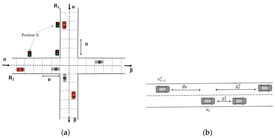
Figure 1.
(a) The scheme of the intersection; (b) the variables related to lane change.
The position of each vehicle at the next time step () is determined according to a parallel dynamic and using the four following rules of a NaSch model [3]:
- Acceleration: .
- Deceleration: .
- Randomization: , with a braking probability .
- Movement: .
where and denote the speed and position of the i-th vehicle, respectively, at the time-step t. is the number of empty sites in front of the i-th vehicle.
Furthermore, open boundary conditions are used, where vehicles can move into or get out of each road with an injection rate and extraction rate , respectively. At the first cell, a vehicle with speed 0 is created with the rate . At the end of the system, if the new position of the vehicle exceeds the length of the road, the vehicle leaves the system with a rate of , otherwise, the vehicle reduces its speed to stay in the system. Furthermore, at the entry, slow (fast) vehicles firstly choose the first cell of the right (left) lane. If it is occupied, they choose the first cell of the left (right) lane if it is empty. Otherwise, they are deleted.
Moreover, the lane-changing process and the absence of lane discipline is an important characteristic of heterogeneous traffic [52], where drivers often change lanes to keep their speed as high as possible or to avoid some incidents on the road.
In the lane-changing model, the rules can be symmetric or asymmetric. The symmetric model considers both lanes, left and right, and all vehicles, slow and fast, equally. Nonetheless, in the asymmetric model, the lane-changing depends on the lane (left and right) and the vehicle (fast or slow). Indeed, in this paper, vehicles can change the lane if the following criteria are satisfied [53]:
For the symmetric model (which corresponds to all vehicles and both lanes):
- ,
- ,
- The adjacent cell in the other lane is empty,
- ,
where and are the gaps in front of the vehicle in the other lane (left or right) and the current lane, respectively. denotes the back gap in the other lane. refers to the maximum speed of the vehicle behind in the other lane (see Figure 1b).
In the asymmetric model, the lane-changing rules depend on the vehicle kind (fast or slow) and the lane (left or right):
- Changing from the left lane to the right lane:In addition to the symmetric conditions, a slow vehicle can change the lane if the gap in front on the right lane is higher than its speed. For a fast vehicle, we adopt the same rules as those of slow vehicles, but it does not shift to the right lane if there is a slow vehicle in front within a distance of in the right lane.
- Changing from the right lane to the left lane:For a slow vehicle, lane-changing rules are the same as those of the symmetric model. Nevertheless, for a fast vehicle, in addition to the symmetric conditions, it can shift to the left lane if there is a slow vehicle within a distance of .
Thus, vehicles can change the lane with the probability if the above lane-changing conditions are satisfied.
2.2. Vehicles’ Emissions
In the literature, there are many traffic emissions models. Some of them use only the speed and vehicle power to calculate the emission [54,55]. Whereas, other models need a lot of vehicle parameters (e.g., engine speed, engine displacement, the coefficient of drag, frontal surface area [56,57]). In this study, we chose the model proposed by Panis et al. [23] for many reasons. Firstly, data of this model take into consideration the traffic heterogeneity: cars, buses, and trucks. Moreover, it allows us to calculate the emission of each vehicle at each iteration based on both its acceleration (positive or negative) and its instantaneous speed. Additionally, Panis et al. [23] showed that this model is appropriate for vehicles’ traffic emission in cities, with a 95% of confidence. Based on empirical measurement and using the non-linear regression technique, they proposed the following general emission function:
where is the instantaneous emission (g/s) of vehicle i. is a lower limit of emission (g/s) for pollutant type and each vehicle. and denote the instantaneous speed (m/s) and instantaneous acceleration (m/s) of the i-th vehicle, respectively. to are the constants of the emission function calculated by the regression analysis, as shown in Table 1. For simplicity, we consider that fast vehicles are petrol cars and slow vehicles are heavy duty vehicles (HDV, diesel) [23].

Table 1.
The constants of the emission function calculated by the regression analysis [23].
2.3. Traffic Intersection and Control Strategies
Generally, at urban intersections, vehicles movement is controlled by traffic lights to ensure safety and smooth traffic flow. In this paper, the traffic intersection is controlled as follows: On the first road , vehicles move from the north to the south, while, on the second road , vehicles move from the east to the west. At the intersection, the traffic flow is controlled by traffic lights. For a period , the road has the priority (green light) and simultaneously receives red light. Afterwards, the light turns green (priority) on for a period (simultaneously, a red light for ). Near the intersection, vehicles without priority reduce their speeds to , where is the position of the intersection.
2.3.1. The First Strategy:
The first strategy is based on double traffic lights in both roads and , located at a position X prior to the intersection (see Figure 1a). This deployment is intended to control the incoming flux. Here, both traffic lights (at the position X and at the intersection) are synchronized, i.e., they have the same period and switch at the same time. On , vehicles arriving at the first traffic light (position X) have priority during a period . Here, the traffic light is in the red period at position X on . Afterwards, the light turns red on and green on at positions X, for the period .
2.3.2. The Second Strategy
The coordination of traffic lights is an EXP-complete problem; therefore, the optimal control of large traffic network is intractable. The mean problem is the non-stationarity of the traffic, where the number of vehicles arriving at intersections changes with the time. This implies that finding optimal control will be effective for a short time [58]. Therefore, self-organizing (adaptation) appears as an alternative solution to this problem [59]. In this work, traffic lights change depending on the traffic characteristics. Thus, the intersection follows the subsequent rules to have an optimal control:
- The number of vehicles within the distance D before the intersection in each road is calculated.
- Then, light must turn green for the road with a higher number of vehicles (simultaneously red for the other road).
- This light remains green for the period .
- If both roads have the same number of vehicles within the distance D, then the priority (green light) is given to one road randomly (i.e., with the probability 0.5).
We called this strategy the self-organizing intersection.
These two strategies are proposed to improve the traffic characteristics, namely, traffic emission and mean speed. Figure 2 depicts the flow chart of this study.
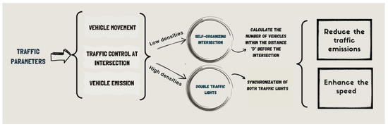
Figure 2.
Flow chart of the experimental design.
The simulation of traffic characteristics was performed using open boundary condition with the following parameters:
- cells,
- and ,
- and ,
- and = 0.8.
The system ran for 50,000 iterations, and we discard the first 40,000 iterations as transient time with 30 independent simulations. The model was programmed using MATLAB 2021b.
3. Results
Let’s start with the first case, where the intersection was controlled by conventional traffic lights.
3.1. Conventional Traffic Lights
Different traffic emissions (CO, PM, VOC, and NO) and vehicle state ratios (stopping , following , deceleration and acceleration), are plotted against the corresponding and in Figure 3.
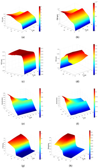
Figure 3.
Different traffic emissions (a–d); acceleration (e–h); deceleration; following and stopping ratios, respectively.
For low values of , CO, and PM, emission increases with until it reaches a maximum value at high injection rates, then it keeps constant. For intermediate and high , this emission exhibits a maximum at intermediate values of , then it shrinks and keeps a constant value. Furthermore, NO emission has the same behavior but presents a maximum at an intermediate value of for all values. In the case of VOC, the emission augments almost linearly with a further increase of until , then it keeps a constant maximum when . Afterwards, it shrinks a little, conserving a constant value.
At low values of , when the injection rate increases (increasing the vehicle number), the interactions among vehicles increase ad well, and the stop and go process takes place, then, the ratio of acceleration and deceleration rises, leading to maximum traffic emission.
Moreover, at low values of , most vehicles follow each other at high speed without congestion. That is why the ratio of following is higher, whereas, the ratios of acceleration, deceleration, and stopping are low (Figure 3e–h), thereby declining traffic emission.
Additionally, for low and intermediate injection rates (), the headway between vehicles is high. As increases, the maximum of CO, PM, and NO emission is situated at intermediate . Here, the headway is reduced because of the stopped vehicles at the intersection, then, acceleration and deceleration ratios exhibit a maximum while the ratio of following shrinks remarkably. Thus, traffic emission increases in increments. Nevertheless, when traffic is dense (), most vehicles stop because of the high density. The augmenting of for one road augments the waiting time of the other road (increases the red light) and makes vehicles stop for more time before the intersection on the other road (). As shown in Figure 3h, the ratio of stopped cars augments. Thus, traffic emission drops. Moreover, vehicles through the intersection can move with a constant speed because of the high free space created after the intersection, hence, traffic emission diminishes. On the other hand, at low and intermediate values of , VOC emission keeps almost the same values with increasing . Nevertheless, the augment of results in a slim increment in VOC emission in the range of large values of (Figure 3d).
Therefore, when traffic is dense, it is better to use large periods of green lights. Otherwise, in the light traffic condition, it is better to reduce the period of switching traffic lights.
From Figure 3a, we can draw the phase diagram of CO emission as a function of and , as shown in Figure 4. The system can be in four different phases depending on the feature changes of the CO emission. In the first phase, the CO emission increases linearly, together with the augment of injection rate. The second phase is characterized by a quasilinear increase of CO emission up to the maximum value with a slop smaller than that of phase I. In phase III, the system keeps constant the maximum value of the CO emission even if with a further increment of . Different from phase III, CO emission first drops and then keeps constant in phase IV. It is worth noticing that the transition from phase II to phase III is the second order, while the transition is the first order from phase II to phase IV.
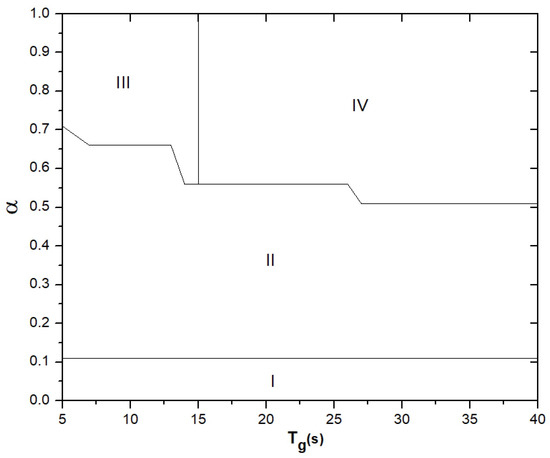
Figure 4.
Phase diagram of the system in the space parameters (, ).
As mentioned before, the lane-changing rules can be symmetric or asymmetric. In the following paragraph, we will discuss the impact of the symmetric model on the traffic emission.
In the asymmetric model (Figure 3a), the augment of results in a high CO emission when . This effect disappears in the case of symmetric model, where the curve of CO emission keeps almost unchanged, as we can see in Figure 5a.
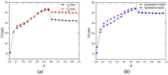
Figure 5.
(a) CO emission as a function of for two values of using the symmetric model. (b) CO emission using the symmetric and asymmetric models, with s.
At high injection rates, as increases, CO emission drops. Furthermore, Figure 5b provides a comparison, in terms of CO emissions, between symmetric and asymmetric models.
In both cases, CO emission shared a similar qualitative trend curve and they reached almost the same maximum. Moreover, CO emission is higher using the asymmetric model at low and intermediate . Here, vehicles (slow and fast) changed lanes more frequently than in the symmetric model [53]. In other words, the acceleration and deceleration processes are presented more frequently in the asymmetric model, which leads to more CO emissions. Nevertheless, at jamming level, the number of lane-changing is almost identical because the headway between vehicles in both lanes is low. Thus, the type of lane changing rules (symmetric or asymmetric) does not affect the CO emission.
Now we raise the question: how we can reduce the CO emissions and enhance the speed, simultaneously?
For this purpose, in the following, we investigate the impact of both strategies proposed in the model.
3.2. Double Traffic Lights
The use of a traffic light before the intersection notably changes the behavior of traffic emission, as shown in Figure 6.
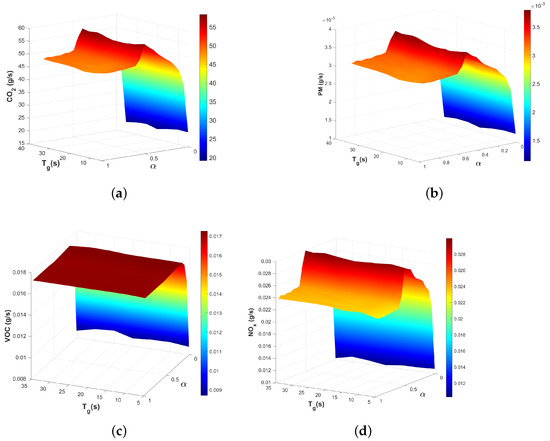
Figure 6.
Different traffic emissions as a function of and , (a) CO, (b) PM, (c) VOC, (d) NO.
In the first strategy, CO emission exhibits a maximum at intermediates values of and high , whereas, in the conventional intersection, the maximum is presented at the high values of and low . Moreover, the minimum is presented when 12 s < < 25 s. It corresponds to the interval with the least acceleration and deceleration process, as illustrated in Figure 7.
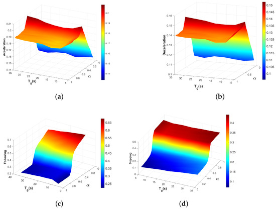
Figure 7.
(a) Acceleration, (b) deceleration, (c) following, and (d) stopping ratios, as a function of and .
The same behavior is observed with the PM emission. The NO emission presents a maximum at high and low , while the maximum is observed at intermediate and high in the conventional intersection. However, this strategy does not affect the VOC emission. The ratio of following cars is almost the same in both cases (Figure 6c). At intermediates and high , this strategy keeps almost constant the number of stopped vehicles in the system. Therefore, this strategy reduces the speed fluctuations (reduces the acceleration and deceleration process), which makes the system more stable, thus, the traffic emission drops.
It is noteworthy that using this strategy augments the number of stooped vehicles and the acceleration deceleration process when traffic is low. Consequently, this strategy can enhance the traffic characteristics only in high traffic conditions in comparison with conventional intersection.
In the following, we discuss the second strategy that can enhance the traffic characteristics in low and intermediates densities.
3.3. Self-Organizing Intersection
This strategy is based on traffic control over a distance D near the intersection.
To choose the best Distance D, the different emissions (CO, VOC, NOX, and PM) were plotted against and D.
As observed in Figure 8, for small distances ( sites), the system shows low emissions of PM and high emissions of CO and NO. For sites, these emissions remain the same. Furthermore, the variation of D has no effect on the VOC emission, where it stays in the same state even if D increases. It is worth noticing that, when sites, the CO and NO emissions can be reduced with 1 g/s and g/s, respectively. Meanwhile, the small distance sites, reduces only the PM emission with g/s; however, NO and CO emissions increase. In other words, the choice of D should neither be too small nor too much. For this reason, the distance sites are used in the rest of the paper.
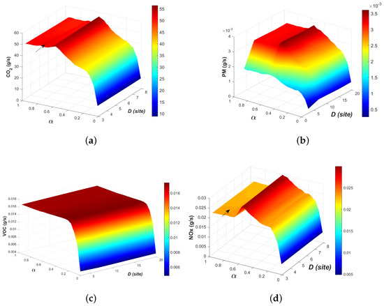
Figure 8.
Different traffic emissions as a function of D and , (a) CO, (b) PM, (c) VOC, (d) NO.
To compare both strategies with conventional intersection, the average speed and CO emissions are plotted against the injection rate in the three cases (see Figure 9).
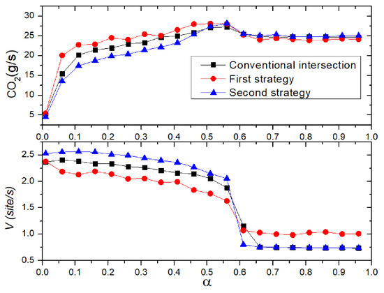
Figure 9.
CO emission and speed as a function of using both strategies and conventional traffic lights. s and sites.
It can be inferred that the speed and CO emissions shared a similar trend curve in the three cases; however, the quantitative behavior is different. There is a critical injection rate, above and after which the effect of each strategy changes. When , it is noticeable that the self-organizing traffic lights strategy impacts on the traffic characteristics and shows the best results in terms of CO emissions and the speed. This strategy enhances the speed and reduces the CO emission simultaneously, which represents a maximum reduction of 13.6% in vehicles’ emission and an increase of 9.5% in the mean speed (comparing the maximum of CO and V with those of the conventional intersection). However, using double traffic lights, the system has the lower speed and higher CO emission. In addition, intersection with conventional traffic lights shows intermediate values of speed and CO emissions in comparison to two other strategies. When traffic is dense (), this situation changes. Intersection with double traffic lights exhibits the best results, because it minimizes CO emissions and maximizes the speed, which represent a mean speed increase up to 28.8% and a reduction in the traffic emissions of 3.6%. Nonetheless, self-organizing traffic lights and conventional traffic lights reduce the speed and slightly increase the CO emissions. Therefore, to promote the traffic efficiency in light and dense traffic conditions, the combination of self-organizing traffic lights and double traffic lights can be used.
To get some further insight into this result, we plotted the average speed in each road site in the three cases (Figure 10).
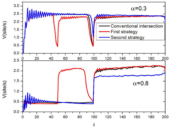
Figure 10.
Speed profile as a function of road sites for two values of using conventional traffic lights and both strategies.
The comparison between the self-organizing intersection and conventional intersection shows that the mean speed in both cases is the same in all sites until site 91 before the intersection. On the one hand, we can observe a clear difference, where the speed with conventional intersection drops noticeably. Nonetheless, the speed keeps high values using the second strategy. On the other hand, the intersection with double traffic lights shows the lower speed profile. One can see that the speed exhibits two drops corresponding to the traffic lights positions. Nevertheless, the situation changes in high densities. The speed profile exhibits lower value, adopting the second strategy.
For a deeper explanation of the CO emission distribution all over the system, Figure 11 and Figure 12 depicts the heatmap of the intersection in the three cases with two values of .
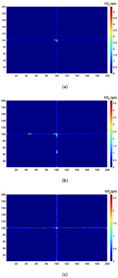
Figure 11.
Heatmap of the intersection: (a) with conventional traffic lights and = 0.2, (b) with the first strategy and = 0.2 and (c) with the second strategy and = 0.2.
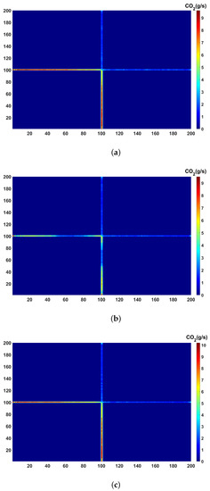
Figure 12.
Heatmap of the intersection: (a) with conventional traffic lights and = 0.8, (b) with the first strategy and = 0.8 and (c) with the second strategy and = 0.8.
In all cases, the high CO emissions are presented before the intersection. However, the emissions after the intersection are low and are due the congestion caused by vehicle density. At low injection rates (Figure 11), the red spots (i.e., indicating high emissions) are a little bit larger in the case of conventional traffic lights compared to the conventional traffic lights and the second strategy. Nonetheless, at high injection rates (Figure 12), using the first strategy, the system shows low CO emission, especially before the intersection.
4. Discussion
Zhao et al. [60] studied the vehicle emissions at an unsaturated intersection using a single-lane road. They found that the increase of the green light duration has a positive effect on reducing traffic emissions. The same result was found by Lv et al. [28]. It is shown that the emission decreases, while the delay increases as the cycle length rises.
However, in our study, for low densities (low injection rate), has no effect. The traffic emission is almost the same for all values of . At intermediate injection rates, traffic emission increases with augmenting . Nonetheless, when the traffic is dense, augmenting can reduce the traffic emissions. Thus, the effect of green signal length strongly depends on the traffic density.
This difference is due to the fact that, in the previous models, they used a single-lane road and the density effect was not considered. Moreover, they calculated the vehicle emissions in only one road of the intersection. However, in our model, we take into consideration all cases of traffic state; from the very low densities to saturated intersection, the impact of lane-changing, and the traffic state in the four legs of the intersection, which gives us a better idea about traffic emission behavior as a function of different traffic related parameters.
The optimization of the traffic lights cycle is widely used to decrease vehicular emissions at intersections. Jin and Lei [30] showed that the optimized model based on fixed time can enhance only the traffic mobility. Zhao et al. [32] showed that the optimization of signal timing from the perspective of CO emission is different from that of the delay control. Optimized fixed cycle time of traffic lights cannot enhance the traffic flow and reduce emissions at the same time. Nevertheless, in our model, the proposed strategies have a positive impact on both perspectives.
It is very difficult to use only one strategy to optimize traffic characteristics for all traffic states. The traffic control at the intersection must be adapted depending on traffic related parameter and especially the density.
The first strategy proposed in this paper (double traffic lights) was used in the congested phase, while the self-organizing intersection (second strategy) was used for the free flow phase.
The self-organizing intersection takes into consideration the short interactions among vehicles of both roads at the intersection and gives the priority to the road with high density at a distance D before the intersection, thus, it helps to reduce the vehicle queues.
At low injection rates, vehicles are separated by large distances (high headway) and they can move at high speeds. Using double traffic lights leads to the formation of platoons behind each one, thus the speed decreases. Nonetheless, at high injection rates, using the first strategy, the first traffic lights reduce the number of arriving vehicles at the intersection, which is beneficial to clear the vehicle queues behind the intersection and avoid large congestion. Consequently, at high traffic volume, forcing vehicles to wait for more time can enhance traffic characteristics; slower has a faster effect [61,62]. A similar effect was observed with the speed limit. Pan et al. [48] showed that the impact of speed limit depends strongly on the density. High speed limit has a positive effect on the vehicular emission at low densities. However, low speed limit is better as the traffic becomes more congested.
Most vehicular emissions are produced before the intersection because of the acceleration and deceleration processes due to the traffic lights.
At low injection rates, CO emissions are a little bit larger in the case of conventional traffic lights compared to the second strategy. Nonetheless, the difference is more noticeable with double traffic lights, where high emissions are localized at both traffic lights (on both roads), which indicate that this strategy is not appropriate for low densities. At high injection rates, the second strategy and conventional traffic lights show almost the same CO emission level. Furthermore, all sites before the intersection are characterized by high CO emissions. Nevertheless, using the first strategy, legs before the intersection exhibit generally low CO emission and especially between both traffic lights, due to the free space created by the first traffic lights. Moreover, the investigation of vehicular traffic using autonomous vehicles has received the attention of many scholars. They have been looked at as an effective way to solve traffic-related problems. Li et al. [63] studied the control of traffic intersections with autonomous vehicles using a Genetic algorithm. Simulation results showed that the algorithm can reduce the intersection average travel time delay by 16.3% to 79.3%, depending on the demand scenario. Moreover, connected vehicles can reduce greenhouse gas emissions by 35% [64]. We believe that autonomous vehicles have a significant effect on traffic characteristics and can reduce vehicle emissions at intersections. One of the advantages of this study is that the autonomous vehicles can be implemented in the proposed model to investigate their effect on the traffic characteristics at the intersection.
5. Conclusions
We proposed a cellular automata model to simulate the traffic characteristics, namely traffic emissions and mean speed, at a signalized intersection. The model is intended to isolate the parameters involved in vehicle-vehicle interactions (lane changing, acceleration, speed, density, and traffic heterogeneity) to improve the comprehension of the signalization effects by analyzing the resultant emissions. Three main elements were considered in this model: vehicle movement (NaSch model and lane-changing rules), traffic control at intersection, and vehicle emission. The results suggest that to decrease the traffic emissions at conventional intersection, the green light duration should be increased when traffic is dense and reduced in light traffic conditions. Moreover, the phase diagram in the space parameters (, ) shows that the system can be in four different phases. The transition from phase II (I) to phase III (II) is the second order, while the transition is the first order from phase II to phase IV.
This paper is an attempt at trying to overcome the following limitations, among others, existing in the previous works:
- The traffic emissions were studied without any improvement suggestion.
- The proposed optimization methods can reduce the traffic emissions at low or high densities and not at both. Additionally, some algorithms can improve the flow and do not reduce emissions and vice versa.
- In the framework of cellular automata, there is a lack of models of traffic emission at intersections.
For this reason, we proposed two strategies, double traffic lights and self-organizing traffic lights, to optimize traffic characteristics. The first strategy was based on the use of traffic lights before the intersection to control the traffic arriving flux at the intersection. The second strategy was the self-organizing traffic lights, where the traffic lights switch depending on the traffic state of each road near the intersection. The first strategy can enhance the mean speed up to 28.8% and reduce the traffic emissions by 3.6% at high values of . However, at low and intermediate , the second strategy shows a maximum reduction of 13.6% in vehicles’ emission and an increase of 9.5% in the mean speed. Therefore, the combination of both strategies can promote the traffic efficiency at all traffic conditions. Finally, it is found that the traffic emission is likely to decrease using the symmetric lane-changing rules. The finding results can be used to better understand how different traffic-related parameters can affect vehicular emission for better optimization.
Author Contributions
Conceptualization, R.M., N.L. and J.R.P.C.; Formal analysis, R.M.; Funding acquisition, R.M.; Investigation, R.M. and C.J.V.G.; Methodology, R.M.; Project administration, R.M.; Resources, C.J.V.G.; Software, R.M.; Supervision, R.M., N.L. and J.R.P.C.; Validation, R.M., N.L. and J.R.P.C.; Visualization, R.M.; Writing—original draft, R.M.; Writing—review & editing, R.M., N.L., J.R.P.C. and C.J.V.G. All authors have read and agreed to the published version of the manuscript.
Funding
This research received no external funding.
Data Availability Statement
Not applicable.
Conflicts of Interest
The authors declare no conflict of interest.
References
- Lighthill, M.J.; Whitham, G.B. On kinematic waves II. A theory of traffic flow on long crowded roads. Proc. R. Soc. Lond. Ser. Math. Phys. Sci. 1955, 229, 317–345. [Google Scholar]
- Daganzo, C.F. The cell transmission model: A dynamic representation of highway traffic consistent with the hydrodynamic theory. Transp. Res. Part B Methodol. 1994, 28, 269–287. [Google Scholar] [CrossRef]
- Nagel, K.; Schreckenberg, M. A cellular automaton model for freeway traffic. J. Phys. I 1992, 2, 2221–2229. [Google Scholar] [CrossRef]
- Moussa, N. Dangerous Situations In Two-Lane Traffic Flow Models. Int. J. Mod. Phys. C 2005, 16, 1133–1148. [Google Scholar] [CrossRef]
- Lakouari, N.; Oubram, O.; Bassam, A.; Pomares Hernandez, S.E.; Marzoug, R.; Ez-Zahraouy, H. Modeling and simulation of CO2 emissions in roundabout intersection. J. Comput. Sci. 2020, 40, 101072. [Google Scholar] [CrossRef]
- Marzoug, R.; Lakouari, N.; Ez-Zahraouy, H.; Castillo Téllez, B.; Castillo Téllez, M.; Cisneros Villalobos, L. Modeling and simulation of car accidents at a signalized intersection using cellular automata. Phys. A Stat. Mech. Its Appl. 2022, 589, 126599. [Google Scholar] [CrossRef]
- National Research Council. Expanding Metropolitan Highways: Implications for Air Quality and Energy Use; National Academy Press: Washington, DC, USA, 1995. [Google Scholar]
- Cavender, J.H.; Kircher, D.S.; Hoffman, A.J. Nationwide Air Pollutant Emission Trends, 1940–1970; US Environmental Protection Agency, Office of Air Quality Planning and Standards: Washington, DC, USA, 1973.
- Escap, U. Using Smart Transport Technologies to Mitigate Greenhouse Gas Emissions from the Transport Sector in Asia. 2019. Available online: https://repository.unescap.org/handle/20.500.12870/344 (accessed on 1 January 2022).
- Hoek, G.; Brunekreef, B.; Goldbohm, S.; Fischer, P.; van den Brandt, P.A. Association between mortality and indicators of traffic-related air pollution in the Netherlands: A cohort study. Lancet 2002, 360, 1203–1209. [Google Scholar] [CrossRef]
- Pope, C.A., III; Burnett, R.T.; Thun, M.J.; Calle, E.E.; Krewski, D.; Ito, K.; Thurston, G.D. Lung Cancer, Cardiopulmonary Mortality, and Long-term Exposure to Fine Particulate Air Pollution. JAMA 2002, 287, 1132–1141. [Google Scholar] [CrossRef]
- Ahn, K. Microscopic Fuel Consumption and Emission Modeling. Ph.D. Thesis, Virginia Tech, Blacksburg, VA, USA, 1998. [Google Scholar]
- Akcelik, R.; Besley, M. Operating cost, fuel consumption, and emission models in aaSIDRA and aaMOTION. In Proceedings of the 25th Conference of Australian Institutes of Transport Research (CAITR 2003), University of South Australia Adelaide, Adelaide, Australia, 3–5 December 2003; pp. 1–15. [Google Scholar]
- Rakha, H.; Ahn, K.; El-Shawarby, I.; Jang, S. Emission model development using in-vehicle on-road emission measurements. In Proceedings of the Annual Meeting of the Transportation Research Board, Washington, DC, USA, 10–14 January 2004; Volume 2. [Google Scholar]
- De Vlieger, I. On board emission and fuel consumption measurement campaign on petrol-driven passenger cars. Atmos. Environ. 1997, 31, 3753–3761. [Google Scholar] [CrossRef]
- De Vlieger, I.; De Keukeleere, D.; Kretzschmar, J. Environmental effects of driving behaviour and congestion related to passenger cars. Atmos. Environ. 2000, 34, 4649–4655. [Google Scholar] [CrossRef]
- Sturm, P.J.; Pucher, K.; Sudy, C.; Almbauer, R.A. Determination of traffic emissions—Intercomparison of different calculation methods. Sci. Total Environ. 1996, 189–190, 187–196. [Google Scholar] [CrossRef]
- Trozzi, C.; Vaccaro, R.; Crocetti, S. Speed frequency distribution in air pollutants’ emissions estimate from road traffic. Sci. Total Environ. 1996, 189–190, 181–185. [Google Scholar] [CrossRef]
- Hickman, J.; Hassel, D.; Joumard, R.; Samaras, Z.; Sorenson, S. Methodology for Calculating Transport Emissions and Energy Consumption. 1999. Available online: https://trid.trb.org/view/707881 (accessed on 1 January 2022).
- Scora, G.; Barth, M. Comprehensive modal emissions model (cmem), version 3.01. User Guid. Cent. Environ. Res. Technol. Univ. Calif. Riverside 2006, 1070, 1580. [Google Scholar]
- Rakha, H.; Ahn, K.; Trani, A. Development of VT-Micro model for estimating hot stabilized light duty vehicle and truck emissions. Transp. Res. Part D Transp. Environ. 2004, 9, 49–74. [Google Scholar] [CrossRef]
- El-Shawarby, I.; Ahn, K.; Rakha, H. Comparative field evaluation of vehicle cruise speed and acceleration level impacts on hot stabilized emissions. Transp. Res. Part D Transp. Environ. 2005, 10, 13–30. [Google Scholar] [CrossRef]
- Int Panis, L.; Broekx, S.; Liu, R. Modelling instantaneous traffic emission and the influence of traffic speed limits. Sci. Total Environ. 2006, 371, 270–285. [Google Scholar] [CrossRef]
- Kakooza, R.; Luboobi, L.; Mugisha, J. Modeling Traffic Flow and Management at Un-signalized, Signalized and Roundabout Road Intersections. J. Math. Stat. 2005, 1, 194–202. [Google Scholar] [CrossRef]
- Advantages of Traffic Signals. Available online: https://www.cityofirvine.org/signal-operations-maintenance/advantages-traffic-signals (accessed on 4 October 2022).
- Madireddy, M.; De Coensel, B.; Can, A.; Degraeuwe, B.; Beusen, B.; De Vlieger, I.; Botteldooren, D. Assessment of the impact of speed limit reduction and traffic signal coordination on vehicle emissions using an integrated approach. Transp. Res. Part D Transp. Environ. 2011, 16, 504–508. [Google Scholar] [CrossRef]
- Lv, J.; Zhang, Y. Effect of signal coordination on traffic emission. Transp. Res. Part D Transp. Environ. 2012, 17, 149–153. [Google Scholar] [CrossRef]
- Lv, J.; Zhang, Y.; Zietsman, J. Investigating Emission Reduction Benefit From Intersection Signal Optimization. J. Intell. Transp. Syst. 2013, 17, 200–209. [Google Scholar] [CrossRef]
- Qian, R.; Lun, Z.; Wenchen, Y.; Meng, Z. A Traffic Emission-saving Signal Timing Model for Urban Isolated Intersections. Procedia -Soc. Behav. Sci. 2013, 96, 2404–2413. [Google Scholar] [CrossRef]
- Ma, X.; Jin, J.; Lei, W. Multi-criteria analysis of optimal signal plans using microscopic traffic models. Transp. Res. Part D Transp. Environ. 2014, 32, 1–14. [Google Scholar] [CrossRef]
- Huang, W.J.; Ma, R.G.; Ding, H.; Bai, H.J. Study on Vehicle Cumulative Energy Consumption of Signalized Intersections. In Proceedings of the 14th COTA International Conference of Transportation Professionals, Changsha, China, 4–7 July 2014; pp. 2950–2960. [Google Scholar] [CrossRef]
- Zhao, H.X.; He, R.C.; Yin, N. Modeling of vehicle CO2 emissions and signal timing analysis at a signalized intersection considering fuel vehicles and electric vehicles. Eur. Transp. Res. Rev. 2021, 13, 5. [Google Scholar] [CrossRef]
- Sharma, P.; Chhillar, A.; Said, Z.; Memon, S. Exploring the Exhaust Emission and Efficiency of Algal Biodiesel Powered Compression Ignition Engine: Application of Box–Behnken and Desirability Based Multi-Objective Response Surface Methodology. Energies 2021, 14, 5968. [Google Scholar] [CrossRef]
- Rajamoorthy, R.; Arunachalam, G.; Kasinathan, P.; Devendiran, R.; Ahmadi, P.; Pandiyan, S.; Muthusamy, S.; Panchal, H.; Kazem, H.A.; Sharma, P. A novel intelligent transport system charging scheduling for electric vehicles using Grey Wolf Optimizer and Sail Fish Optimization algorithms. Energy Sources Part Recover. Util. Environ. Eff. 2022, 44, 3555–3575. [Google Scholar] [CrossRef]
- Park, S.; Wagner, D.F. Incorporating cellular automata simulators as analytical engines in GIS. Trans. GIS 1997, 2, 213–231. [Google Scholar] [CrossRef]
- Du, G.; Shin, K.J.; Yuan, L.; Managi, S. A comparative approach to modelling multiple urban land use changes using tree-based methods and cellular automata: The case of Greater Tokyo Area. Int. J. Geogr. Inf. Sci. 2018, 32, 757–782. [Google Scholar] [CrossRef]
- Bhattacharjee, K.; Naskar, N.; Roy, S.; Das, S. A survey of cellular automata: Types, dynamics, non-uniformity and applications. Nat. Comput. 2020, 19, 433–461. [Google Scholar] [CrossRef]
- Marzoug, R.; Bamaarouf, O.; Lakouari, N.; Castillo-Téllez, B.; Téllez, M.C.; Oubram, O. Traffic intersection characteristics with accidents and evacuation of damaged cars. Phys. A Stat. Mech. Its Appl. 2021, 561, 125217. [Google Scholar] [CrossRef]
- Foulaadvand, M.E.; Fukui, M.; Belbasi, S. Phase structure of a single urban intersection: A simulation study. J. Stat. Mech. Theory Exp. 2010, 2010, P07012. [Google Scholar] [CrossRef]
- Nagatani, T. Traffic flow stabilized by matching speed on network with a bottleneck. Phys. A Stat. Mech. Its Appl. 2020, 538, 122838. [Google Scholar] [CrossRef]
- Bouderba, S.I.; Moussa, N. Evolutionary dilemma game for conflict resolution at unsignalized traffic intersection. Int. J. Mod. Phys. C 2019, 30, 1950018. [Google Scholar] [CrossRef]
- Marzoug, R.; Lakouari, N.; Oubram, O.; Ez-Zahraouy, H.; Cisneros-Villalobos, L.; Velásquez-Aguilar, J.G. Impact of information feedback strategy on the car accidents in two-route scenario. Int. J. Mod. Phys. C 2018, 29, 1850081. [Google Scholar] [CrossRef]
- Regragui, Y.; Moussa, N. A cellular automata model for urban traffic with multiple roundabouts. Chin. J. Phys. 2018, 56, 1273–1285. [Google Scholar] [CrossRef]
- Salcido, A.; Hernández-Zapata, E.; Carreón-Sierra, S. Exact results of 1D traffic cellular automata: The low-density behavior of the Fukui–Ishibashi model. Phys. A Stat. Mech. Its Appl. 2018, 494, 276–287. [Google Scholar] [CrossRef]
- Marzoug, R.; Ez-Zahraouy, H.; Benyoussef, A. Cellular automata traffic flow behavior at the intersection of two roads. Phys. Scr. 2014, 89, 065002. [Google Scholar] [CrossRef]
- Yang, M.L.; Liu, Y.G.; You, Z.S. Investigation of fuel consumption and pollution emissions in cellular automata. Chin. J. Phys. 2009, 47, 589–597. [Google Scholar]
- Salcido, A.; Carreón-Sierra, S. Air Pollutant Emissions in the Fukui-Ishibashi and Nagel-Schreckenberg Traffic Cellular Automata. J. Appl. Math. Phys. 2017, 5, 2140–2161. [Google Scholar] [CrossRef]
- Pan, W.; Xue, Y.; He, H.D.; Lu, W.Z. Impacts of traffic congestion on fuel rate, dissipation and particle emission in a single lane based on Nasch Model. Phys. A Stat. Mech. Its Appl. 2018, 503, 154–162. [Google Scholar] [CrossRef]
- Xue, Y.; Wang, X.; Cen, B.L.; Zhang, P.; He, H.D. Study on fuel consumption in the Kerner–Klenov–Wolf three-phase cellular automaton traffic flow model. Nonlinear Dyn. 2020, 102, 393–402. [Google Scholar] [CrossRef]
- Wang, X.; Xue, Y.; Cen, B.L.; Zhang, P. Study on pollutant emissions of mixed traffic flow in cellular automaton. Phys. A Stat. Mech. Its Appl. 2020, 537, 122686. [Google Scholar] [CrossRef]
- Singh, M.K.; Ramachandra Rao, K. Cellular automata models for signalised and unsignalised intersections with special attention to mixed traffic flow: A review. IET Intell. Transp. Syst. 2020, 14, 1507–1516. [Google Scholar] [CrossRef]
- Kanagaraj, V.; Asaithambi, G.; Toledo, T.; Lee, T.C. Trajectory Data and Flow Characteristics of Mixed Traffic. Transp. Res. Rec. 2015, 2491, 1–11. [Google Scholar] [CrossRef]
- Chowdhury, D.; Wolf, D.E.; Schreckenberg, M. Particle hopping models for two-lane traffic with two kinds of vehicles: Effects of lane-changing rules. Phys. A Stat. Mech. Its Appl. 1997, 235, 417–439. [Google Scholar] [CrossRef]
- Treiber, M.; Kesting, A.; Thiemann, C. How much does traffic congestion increase fuel consumption and emissions? Applying a fuel consumption model to the NGSIM trajectory data. In Proceedings of the 87th Annual Meeting of the Transportation Research Board, Washington, DC, USA, 13–17 January 2008; Volume 71, pp. 1–18. [Google Scholar]
- Treiber, M.; Kesting, A. Traffic flow dynamics: Data, models and simulation. Phys. Today 2014, 67, 54. [Google Scholar]
- Barth, M.; Younglove, T.; Scora, G. Development of a Heavy-Duty Diesel Modal Emissions and Fuel Consumption Model; California PATH Research Report UCB-ITS-PRR-2005-1; University of California: Berkeley, CA, USA, 2005. [Google Scholar]
- Barth, M.; Boriboonsomsin, K. Real-world carbon dioxide impacts of traffic congestion. Transp. Res. Rec. 2008, 2058, 163–171. [Google Scholar]
- Papadimitriou, C.; Tsitsiklis, J. The complexity of optimal queueing network control. In Proceedings of the IEEE 9th Annual Conference on Structure in Complexity Theory, Amsterdam, The Netherlands, 28 June–1 July 1994; pp. 318–322. [Google Scholar] [CrossRef]
- Gershenson, C. Design and Control of Self-Organizing Systems; CopIt Arxives: Blagnac, France, 2007. [Google Scholar]
- Zhao, H.; He, R.; Jia, X. Estimation and Analysis of Vehicle Exhaust Emissions at Signalized Intersections Using a Car-Following Model. Sustainability 2019, 11, 3992. [Google Scholar] [CrossRef]
- Gershenson, C.; Helbing, D. When slower is faster. Complexity 2015, 21, 9–15. [Google Scholar] [CrossRef]
- Helbing, D.; Mazloumian, A. Operation regimes and slower-is-faster effect in the controlof traffic intersections. Eur. Phys. J. B 2009, 70, 257–274. [Google Scholar] [CrossRef]
- Li, Z.; Pourmehrab, M.; Elefteriadou, L.; Ranka, S. Intersection control optimization for automated vehicles using genetic algorithm. J. Transp. Eng. Part A Syst. 2018, 144, 04018074. [Google Scholar] [CrossRef]
- Massar, M.; Reza, I.; Rahman, S.M.; Abdullah, S.M.H.; Jamal, A.; Al-Ismail, F.S. Impacts of autonomous vehicles on greenhouse gas emissions—Positive or negative? Int. J. Environ. Res. Public Health 2021, 18, 5567. [Google Scholar] [CrossRef] [PubMed]


Publisher’s Note: MDPI stays neutral with regard to jurisdictional claims in published maps and institutional affiliations. |
© 2022 by the authors. Licensee MDPI, Basel, Switzerland. This article is an open access article distributed under the terms and conditions of the Creative Commons Attribution (CC BY) license (https://creativecommons.org/licenses/by/4.0/).