Assessment of Hydrological Extremes for Arid Catchments: A Case Study in Wadi Al Jizzi, North-West Oman

Abstract

The objective of this research was to analyse hydrological variability by conducting an intensive analysis of extreme events, under dry and wet conditions. Drought conditions were assessed using the Standard Precipitation Index (SPI) and Rainfall Anomaly Index (RAI), while the Soil Conservation Service (SCS) method was used to simulate flooding at four stations. The SPI results indicated that the amount of rainfall within the catchment area is near to normal, ranging from 64% to 75%, with some extremely wet exceptions which may cause flash floods. The RAI results also indicated that the amount of rainfall within the catchment area is near to normal, but the extremely wet category obtained the largest percentage (ranging from 36% to 50%) and the very wet category had the lowest percentage (ranging from 9% to 36%). The simulated flooding, using SCS, tended to slightly underestimate the observed streamflow, while the performance showed some weaknesses when the observed flooding was less than 1 m³/s. The Nash–Sutcliffe Efficiency showed higher performance at closer rainfall stations to the outlet, with values of 0.92 and 0.94. Distant stations simulated floods that showed a lower level of efficiency, with values of 0.77 and 0.81. Given the fact that hydrological extremes (dry and wet conditions) are connected, the findings of the two indices and the SCS method are consistent and suitable for monitoring drought and flood events under climate change.

1. Introduction

Extreme hydrological conditions can lead to major natural disasters at global, regional, and catchment scales, resulting in the loss of property, infrastructure, and life, as well as causing poverty. The Sultanate of Oman suffers annual flood events, particularly along coastal areas where the main cities and buildings are located. On the other hand, the country is also suffering a significant regional drought [1]. It is important to provide policy-makers with drought estimates, in terms of severity and duration [2].

Unlike flood frequency, drought only becomes obvious when it causes significant damage [3,4,5]. However, droughts may have long-term adverse effects on the environment, including social and economic aspects [6]. Undoubtedly, the recognition of hydrological extremes in arid climate catchments, as a part of the integrated water resources system, is not well understood and will depend on the level of research, development, and national awareness of the problem’s significance. Furthermore, drought phenomena can be seen in some other indicators, such as rainfall, streamflow, soil moisture content, and ground water level [7].

Based on Kleist (1993), the time scale, duration, frequency, and intensity of droughts become important themes in any drought analysis [7]. Many researchers have studied extreme hydrological conditions in arid regions, particularly during drought events. Recently, a regional study was conducted by El Kenawy et al. (2020), to assess drought in Oman using the Standard Precipitation Index (SPI) and Standardized Precipitation Evapotranspiration Index (SPEI) [1]. The results showed a significant increase of drought severity for the last four decades, at the country level. Ali et al. (2019) achieved accurate drought forecasts at a small scale on three agricultural plots, using a new multi-stage separation model for estimating Standard Precipitation Index (SPI), at 1, 3, 6, and 12 monthly intervals [8]. Similarly, Zhao et al. (2021) indicated that the SPI could better reflect annual and seasonal dry weather and flood changes in the field of study based on long-term grade measurements [9]. Tsesmelis et al. (2022) implemented the SPI to provide accurate results of drought, at a spatiotemporal regional scale, for Greece [10]. To better perceive and characterise agricultural droughts, Łabędzki (2007) used the 1–3 month SPI which greatly assists the drought detection achieved by the 6-month SPI [11]. He recommended the use of more than one index to evaluate drought risk levels. Kourgialas (2021) assessed hydrological events in the north-western part of Crete (Greece) based on the SPI method, between 1960 and 2019 [5]. Interesting correlations were found between groundwater capacity levels and several interrelated factors, such as rainfall, evapotranspiration, soil, available water capacity, and runoff accumulation. Zhai et al. (2010) used the Rainfall Anomaly Index (RAI), Bhalme–Mooley Index (BMI), the Standard Anomaly Index (SAI), and the Palmer Drought Index (PDSI) to highlight local variations in climatic drought and wet conditions in ten catchments, during the period 1961–2005 [12]. Tufaner and Özbeyaz (2020) applied Machine Learning Algorithms to evaluate the Z index of drought phenomena in Palmer, based on observed rainfall and soil moisture data [13].

The Soil Conservation Service (SCS) was used to effectively assess flooding for arid catchments. Abushandi and Merkel (2011) and Abushandi (2016) applied the SCS method to different arid regions in the Middle East [14,15]. However, there are always problems with assessing hydrological behaviour in arid catchments due to hydrological complexities or data acquisition accuracy. In addition, Shadeed and Almasri (2010) applied a GIS-based SCS-CN approach to develop an estimate of four storm surface runoff events in Palestine [16]. The analysis by Alzghoul and Al-husban (2021) indicated that there is a strong correlation between the curve number used in the SCS method and the values obtained from measured runoff and the rainfall depth [17]. El-Hames (2012) applied an empirical method for runoff prediction in arid and semi-arid catchments based on morphological data and SCS-curve number [18]. The results were validated and calibrated from six different countries using a significant number of rainfall events. Al-Ghobari et al. (2020) studied spatial runoff behaviour due to different land cover types, slopes, and maximum retention, as they are the major parameters for SCS [19]. Braud et al. (2016) tried to explain these phenomena by presenting European and international flood warning systems [20]. The rainfall depth is calculated by the reverse implementation of the hydrological model, based on iterative rainfall inputs to obtain flood peaks. Furthermore, anthropogenic influences were studied by Karagiorgos et al. (2016). They analysed the vulnerability components, including physical and social factors, due to unexpected flooding [21]. The analysis was based on a review of the disability assessment and focused on weaknesses as a framework for outlining and evaluating the negative impact. Mahmood et al. (2017) used daily hydrological data for the years 2013 and 2014, to understand the characteristic distribution of storm rainfall [22].

An estimation of flash flooding in the Wadi Al Jizzi catchment by Abushandi and Al Sarihi (2022), using two different lumped models, showed that a statistical readjustment was needed to avoid underestimation of the small flood values [23]. On the other side of Oman, Al Ruheili et al. (2019) estimated flood damage in the floodplain in the southern part of Oman under current and future conditions [24]. They also determined the flood extent and amount of flood damage using the 3Di model for the year 2002 cyclone (ARB01). While the study gives an overview of the political decisions contributing to the sustainable development of resources, future assessment of the flood damage at catchment scales was also performed.

Further research was based on the integrated implementation of lumped and distributed hydrologic models. Recently, Niyazi et al. (2020) evaluated the runoff compensation equivalent using two models dealing with morphological parameters and hydrological properties [25]. In addition, these models include the Watershed Modelling System (WMS) and the Hydrological Modelling System (HEC-HMS). In addition, Saber et al. (2015) developed physics-based hydrological models adapted to flash floods, to help understand hydrological processes and cope with water-related issues, such as the scarcity of water and data [26]. An ecological assessment for a suggested distributed model of a river basin, in which the wadi system (Hydro-BEAM-WaS) is coupled with remote sensing data, performed well in the absence of high-quality ground observations. However, El Alfy (2016) used a comprehensive approach to assess the effects of floods in urban areas, integrating distributed models and forecast precipitation [27]. The flow model was developed as an activity for capturing objects with daily precipitation measurements. The study showed that rapid urbanisation has a negative impact on the hydrological process, as the sprawl of alluvial channels is important. Jodar-Abellan et al. (2019) evaluated hydrological responses using geographic information system tools (SWAT) in five basins of the Mediterranean (south-eastern Spain) with pixel units from 10.2 to 200.9 km² [28]. Furthermore, Aghabeigi et al. (2020) compared the IHACRES model (Identification of unit Hydrographs And Component flows from Rainfall, Evaporation, and Streamflow data) to the Complex SWAT model for three watersheds: one dry and two semi-dry [29]. The SWAT model performed better than the IHACRES model for some climate zones. Moreover, Abushandi and Merkel (2013) simulated a single flood event in the northern part of Jordan, that occurred in the year 2008, using two models: HEC-HMS and IHACRES, at an hourly scale [30]. An integrating satellite reconnaissance to generate rainfall data (GSMaP_MVK +) was used. The performance of the IHACRES lumped model had some errors, while the calibrated runoff results had a good level of performance in the distributed HEC-HMS.

The Wadi Al Jizzi arid catchment in the northern part of Oman experiences extreme rainfall storms and irregular flash floods due to topographical, climatological, and hydrological complexities. This, however, destroys the infrastructure of the city at the outlet of the catchment, arousing the need for an improved understanding of flood behaviour at a catchment scale. Although the water is limited, the Wadi Al Jizzi catchment is particularly sensitive to flash flooding due to the following field survey findings:

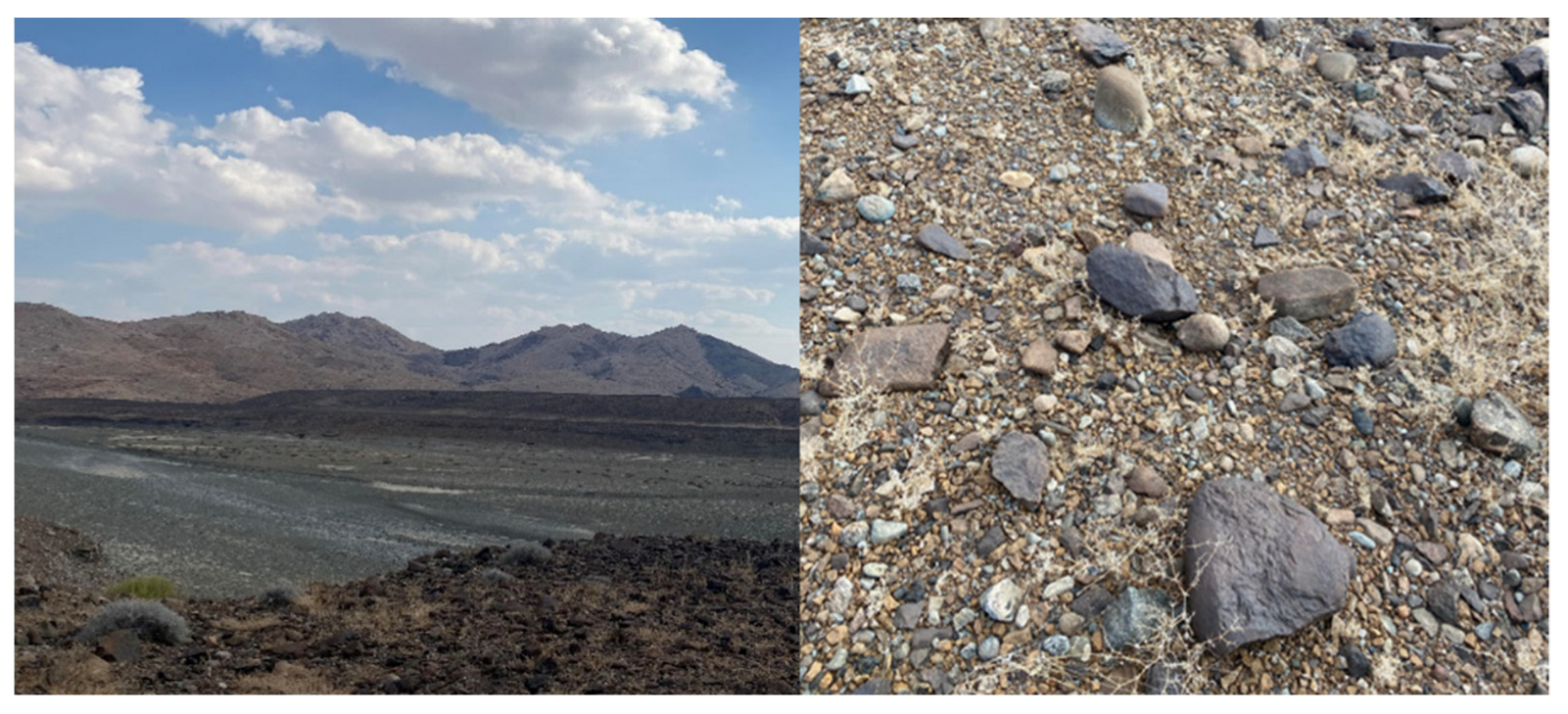
• A series of basaltic mountains surrounding the catchment from the western part, known as Al Hajar Al Gharbi.
• Hyper arid catchment characteristics, including a limited number of high-intensity, annual storm rainfall events in a short time.
• The catchment is dominated by bare soil and very limited vegetation cover.

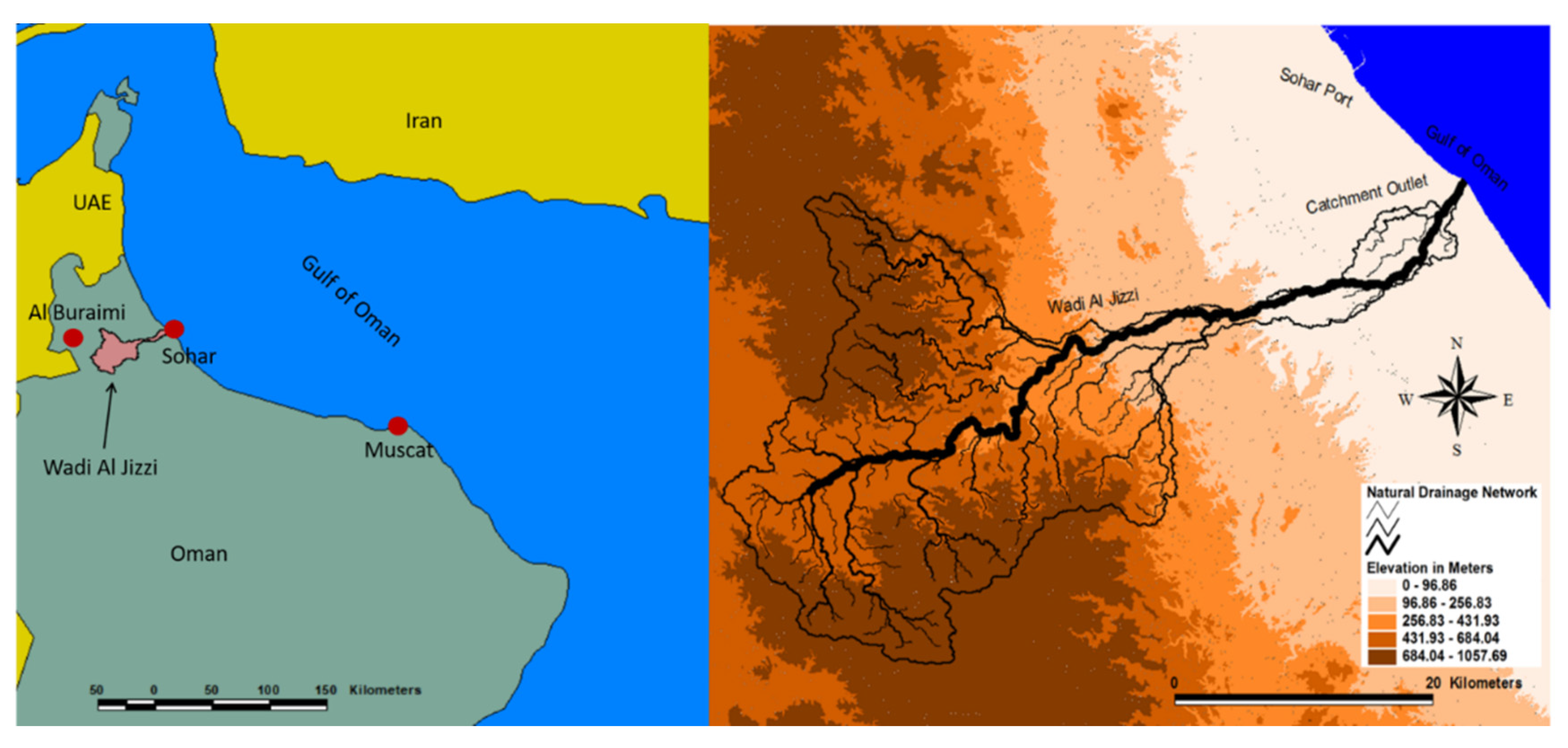
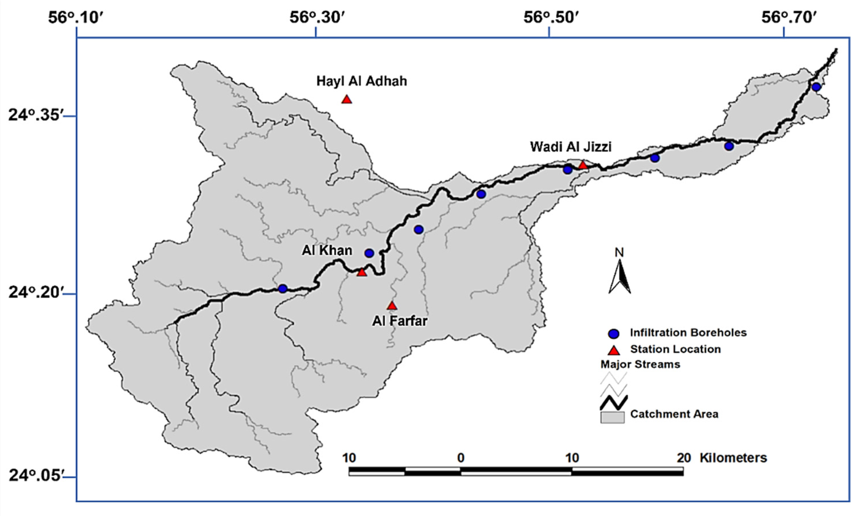
For the better planning, operation, and development of water, energy, and food production, an understanding of extreme hydrologic conditions at a regional scale is an important step. The shortage of both surface and ground water resources controls the difficulties of present and future agricultural activities. Changing the negative impact of flash floods into a fruitful source of water has not been achieved in many areas of Oman. In fact, the main portion of flood water flows into the sea, after destroying the infrastructure. The SPI and RAI methods were successfully applied to arid areas where the observed hydrologic dataset is limited. While both methods are characterised by uncomplicated generic structures, the SCS-CN requires more inputs to simulate wet seasons. Substantial storm rainfall occurred in the upper part of Wadi Al Jizzi, causing serious damage to the infrastructure of Sohar City, located at the catchment outlet. Furthermore, the frequency of flash flooding has dramatically increased over the last 20 years and requires urgent action. However, only a few studies have been conducted to investigate hydrologic wet and drought severities in Oman. The aim of this research is to assess the behaviour of the extreme drought and wet conditions in Wadi Al Jizzi, using the SPI and RAI for drought evaluation and the SCS-CN model for wet seasons.

2. Study Area

The catchment considered in this study is the Wadi Al Jizzi in the North Al Batina Governorate in Oman, alongside the Sohar–Al Buraimi city highway and with a length of 77.8 km. Wadi Al Jizzi represents a major valley in the region and ends in the Sohar coastal outlet. The catchment area is around 870.5 km², with an average slope of 0.56%. The highest mountain around the catchment is more than 1000 m above sea level (Figure 1).

Sohar is the major city located at the outlet of the Wadi Al Jizzi catchment, an area of important crop production. Since the introduction of mechanical pumps, the development of agricultural land has increased since the early 1970s.

There are many villages near Wadi Al Jizzi: some of them belong to Sohar City, and some to Al Buraimi City. The villages belonging to Sohar are Al-Jahili, Al-Huwailat, Sahban, Al-Farfar, Al-Khan, Al-Suhaila, Dhahran, Al-Arja, and others. The state of Buraimi includes the villages of Al-Swadif, Al-Hail, Al-Rabi, Al-Wasit, Katana, Al-Daqiq, and others. The major activity in these villages is agriculture and the water resource is groundwater [31].

The Wadi Al Jizzi catchment is characterised by the presence of many types of impermeable basaltic rocks (Figure 2), the most important of which are igneous rocks, which were formed between 800 million years ago until the present [32]. Sedimentary and metamorphic rocks are present in the region, as sediments of different ages were deposited and then experienced several folding and cracking periods [33]. The soil type is mainly loamy soil with small portions of sandy soil and clay, based on the physical tests conducted. The catchment has only one dam, with an area of 2.7 km², a length of 1350 m, a height of 14 m, and a maximum volume of 5.4 × 106 m³ [34]. There were two purposes for constructing this dam:

• To recharge the ground water which has a water table level of 172 m underground, and
• To protect Sohar City from flash floods during wet seasons.

Generally, the area is considered as being a hyper arid, coastal area: hot and humid during the summer, with an average temperature of 37 °C, and moderate in winter, with an average temperature of 18.5 °C, except for highly elevated land, where the climate remains mild throughout the entire year [35].

Localised thunderstorms occur high over the Al Hajar Al Gharbi Mountain range, in the north of Oman, during the summer months and irregular droughts sweep across the Arabian Peninsula. Rain occurs inland and on the coastal regions in the winter. Rainfall is highly variable from one location to another and from one year to another. Orographic impacts are sometimes affected by local patterns. The amount of surface runoff depends on rainfall intensity and frequency. Apart from some short periods of data loss, records of the wadi runoff since 1984 are both efficient and complete. The runoff of surface water mostly happens between January and April, which are the wet months. Such records are relevant and could be used in statistical predictions. The catchment under study is classified as an ephemeral stream where any water flow within the major wadi catchment is considered as being in flood. The magnitudes of the flooding have been categorised as low, medium, and high.

3. Methodology

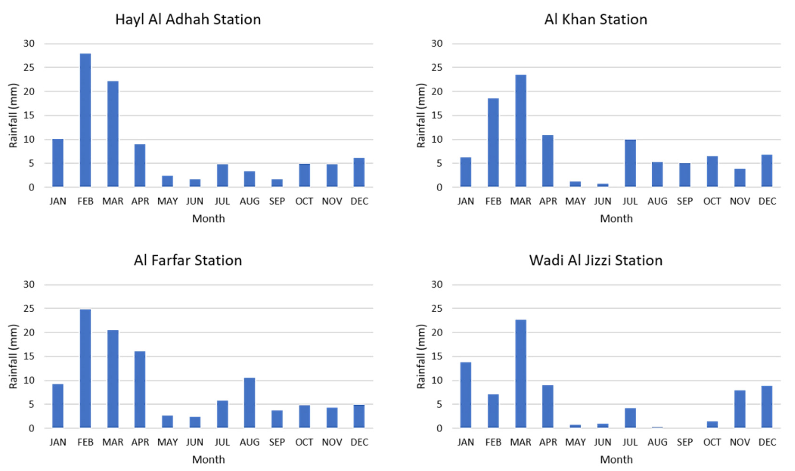
3.1. Rainfall and Runoff Data

Rainfall data are very limited within the catchment area. To conduct any accurate hydrological analysis, continuous long-term rainfall data are required. In this research, four meteorological stations were selected to provide daily rainfall rates collected from the Ministry of Regional Municipal and Water Resource in Oman (

Table 1. Summary of selected meteorological stations.

Elevation Above Sea Level (m)	Annual Rainfall	Acquisition Period	Station Name
524	99.0	1947–2017	Hayl Al Adhah
364	98.4	1982–2017	Al Khan
534	110.0	1974–2016	Al Farfar
459	98.6	1993–2017	Al Jizzi (Near the Dam)

). The average annual rainfall varies from 98.4 mm (in Al Khan station) to 110 mm (in Al Farfar station), while the average annual rainfall for the entire catchment is approximately 101 mm. The recorded data periods of rainfall range from 24 years to 70 years. Figure 3 shows the monthly rainfall distribution for the selected stations.

The maximum daily rainfall of 248 mm was recorded in Hayl Al Adhah station in the year 1988. The next highest daily value (242 mm) occurred in Al Khan station in the year 1996. However, there seems to be no clear influence on which month the maximum rainfall may occur. The highest twenty daily rainfall rates (greater than 110 mm) were recorded in all the stations at no specified months. A Pearson correlation was conducted to test the relationship between maximum daily rainfall rates and showed a moderate relationship between the stations, with an average of 0.66 indicating localised storm events in space and time. The average standard deviation of daily rainfall was about 16.5. The area also commonly experiences several years with very limited or no rainfall. Approximately 12% of the stations’ records are affected by missing rainfall intervals. To bridge the gaps in data acquisition periods between the four locations, a similarity analysis using cross-correlation was implemented.

Furthermore, 26 observed ephemeral runoff events from the Sallan monitoring station were used for validation purposes (Figure 4), using differential pressure flowmeters located at the outlet areas, between the years 1987 and 2007. The number of runoff records ranges from one to four events per year, with an average of 1.3 per year. The individual runoff is characterised by a sharp rise, to generate a narrow hydrograph and short time lags, depending on soil antecedent conditions and rainfall intensity, in addition to the topographic features.

Additionally, soil types were determined using double ring infiltration tests, conducted at eight points within the catchment area, as shown in Figure 5.

In this research, a comparative analysis was conducted to understand drought conditions. The SPI and RAI were used as they are the most extensively used drought indices for hydrologic monitoring, water resource management, and drought prediction. Using two well-reviewed indices should ensure the results’ accuracy.

3.2. Standard Precipitation Index (SPI)

The Standard Precipitation Index (SPI) has been used by many meteorologists and climatologists all over the world for many years. Simple indices such as ‘percentage of normal precipitation’ and ‘precipitation percentage’ were used, as well as more complicated indices such as the Palmer Drought Severity Index. The American scientists McKee, Doesken, and Kleist developed the Standard Precipitation Index (SPI) in 1993, after realising that a lack of precipitation has different effects on underground water, groundwater storage, moisture levels, precipitation, and streamflow. However, all methods performed in this field have a single target, which is to identify the extreme scarcity of rainfall in a particular area. For the purpose of analysing extreme hydrological changes, the Standard Precipitation Index (SPI) was utilised. The equation for determining SPI is:

$$SPI=\frac{x_i-\overline{x}}{S}$$

(1)

where x_i is the monthly precipitation, $\overline{x}$ is the average precipitation, and S is the standard deviation, while:

$$S=\frac{x_i-\overline{x}}{\overline{x}}.$$

(2)

Based on SPI values, the climate can be classified into one of seven classes, as in

Table 2. Climatic classification according to the SPI values [7].

SPI Value	Category
SPI ≥ 2.00	Extremely wet
1.50 ≤ SPI ≤ 1.99	Severely wet
1.00 ≤ SPI ≤ 1.49	Moderately wet
−0.99 ≤ SPI ≤ 0.99	Near normal
−1.49 ≤ SPI ≤ −1.00	Moderately dry
−1.99 ≤ SPI ≤ −1.50	Severely dry
SPI ≤ −2.00	Extremely dry

. The classification is based on monthly rainfall values per year, over four selected station periods.

3.3. Rainfall Anomaly Index (RAI)

According to Costa and Rodrigues (2017), the Rainfall Anomaly Index (RAI) was developed by Rooy in the year 1965 and it uses a classification procedure to assign measures for positive and negative precipitation classes [36]. The RAI considers two types of anomalies: positive and negative. The equations for RAI are:

$$RAI=3\left[\frac{N-\overline{N}}{\overline{M}-\overline{N}}\right]forpositiveanomalies$$

(3)

$$RAI=-3\left[\frac{N-\overline{N}}{\overline{x}-\overline{N}}\right]fornegativeanomalies$$

(4)

where:

• N = Current monthly/yearly rainfall (mm),
• $\overline{N}$ = Monthly/yearly average rainfall of the historical series (mm),
• $\overline{M}$ = Average of the ten highest monthly/yearly precipitations of the historical series (mm), and
• $\overline{x}$ = Average of the ten lowest monthly/yearly precipitations of the historical series (mm).

Based on the RAI values, the climate will be classified into one of six classes, as in

Table 3. Climatic classification according to the RAI values [37].

Criterion	Classifications of RAI Intensity
Above 4	Extremely wet
2 to 4	Very wet
0 to 2	Wet
−2 to 0	Dry
−2 to −4	Very dry
Below −4	Extremely dry

. The classification is based on monthly rainfall values per year, over four selected station periods.

3.4. Soil Conservation Service-Curve Number (SCS-CN) Method

The method of the SCS-curve number is simple, commonly used, and an efficient way of determining the estimated amount of runoff from rainfall in a specific area. Although the method is intended for individual storm events [30,38,39], the average annual runoff values can be downscaled [40]. For this method, the input datasets are very small (i.e., precipitation quantity and curve number). Moreover, the SCS method depends on the treatment, hydrological conditions, the soil hydrological group, and land use of the area, as follows:

$$Q=\frac{{\left(P-I_a\right)}^2}{\left(P-I_a\right)+S}$$

(5)

$$I_a=0.2S$$

(6)

$$Q=\frac{{\left(P-0.2S\right)}^2}{\left(P-0.8S\right)}$$

(7)

$$S=\frac{1000}{\mathrm{CN}}-10$$

(8)

where:

• Q = Runoff depth (mm),
• P = Rainfall (mm),
• I_a = Initial abstraction (mm),
• S = Maximum retention after runoff begins (mm × 25.4 to convert from inches),
• CN = Curve number, and

Basic descriptive inputs must be efficiently converted into numeric values of CN, reflecting the catchment runoff potential in the empirical SCS-CN model of hydrological abstraction. The method considers the major characteristics of runoff-producing catchments, such as soil type, land cover type, surface condition, and antecedent soil moisture conditions, in order to determine CN values.

The Nash–Sutcliffe Efficiency was used to evaluate the good fit of simulated runoff using the SCS method, in comparison to the observed runoff:

$$\mathrm{NSE}=1-\frac{{{\displaystyle \sum }}_{t-1}^T{\left(Q_m-Q_o\right)}^2}{{\left(Q_o-{\overline{Q}}_o\right)}^2}$$

(9)

• $Q_m$ = Simulated runoff using SCS method (m³/s),
• $Q_o$ = Observed runoff records (m³/s), and
• ${\overline{Q}}_o$ = Average observed runoff (m³/s).

Pearson correlation was used to find the relationships between several data types, such as observed runoff in comparison with simulated runoff, and different drought classes of RAI and SPI. In addition, the impact of the station’s elevation above sea level on average rainfall was also tested using the Pearson correlation.

4. Results and Discussion

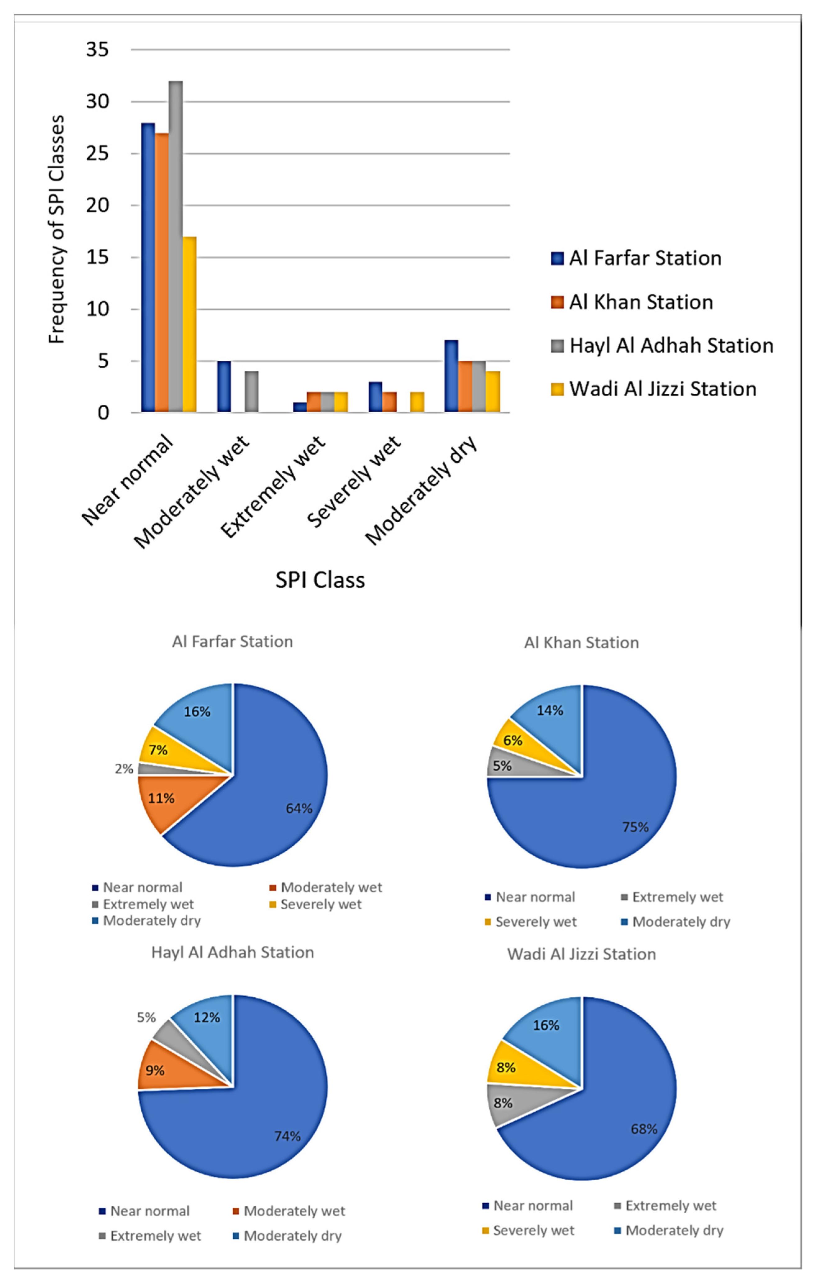
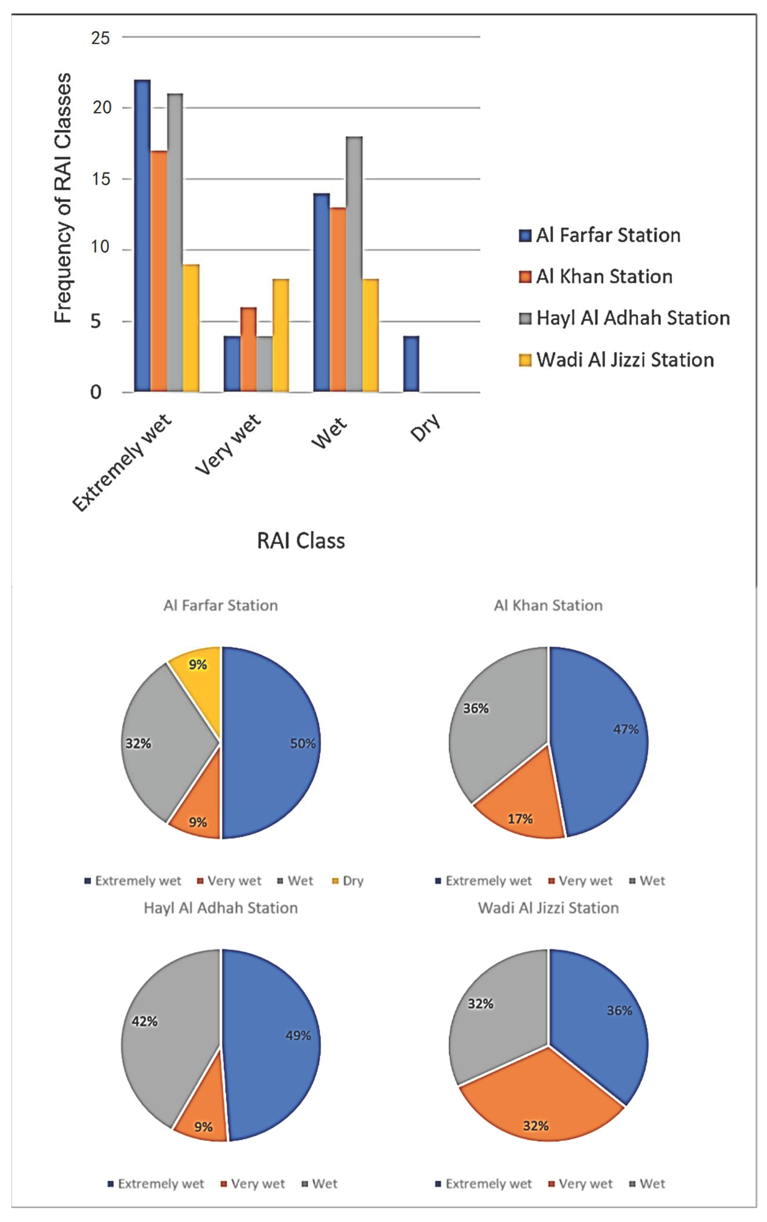
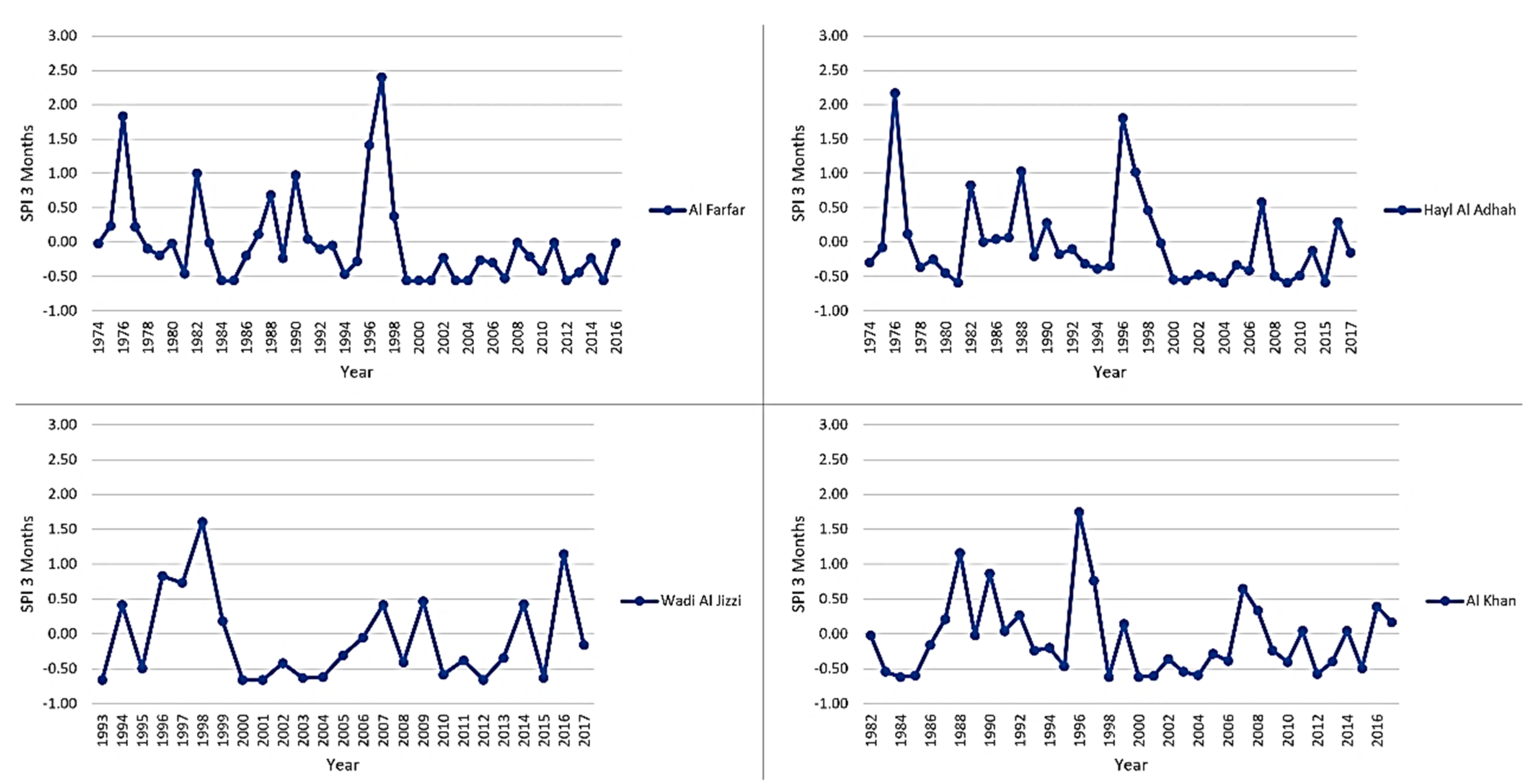
4.1. Drought Indices Analysis

All rainfall data were classified into categories ranging from extremely wet to extremely dry. The maximum SPI at a monthly basis (SPI1) value for Hayl Al Adhah Station was 5.46 in May 1977, while the minimum SPI1 value was −0.65 in March and April (for 18 times in 39 years). However, the maximum SPI1 value for Al Khan Station was 5.27 in July 1995, while the minimum SPI1 value was −0.87 in March (for 12 times in 36 years). Furthermore, the maximum SPI1 value for Al Farfar Station was 5.85 in July 1995, while the minimum SPI1 value was −0.66 in April (for 21 times in 43 years). The maximum SPI1 value for Wadi Al Jizzi Station was 4.1 in July 1995, while the minimum SPI1 value was −0.82 in March (3 times in 25 years). It is worth mentioning that the average maximum SPI1 value was 4.04, while the average minimum SPI1 was −0.69.

Table 4. Maximum and minimum SPI monthly interval values for each meteorological station.

Station Name	SPI Boundary	January	February	March	April	May	June
Hayl Al Adhah	Maximum	4.55	4.32	2.83	3.18	5.46	5.22
	Minimum	−0.59	−0.55	−0.65	−0.65	−0.29	−0.29
Al Khan	Maximum	4.51	4.51	2.82	4.19	2.77	5.27
	Minimum	−0.44	−0.35	−0.57	−0.45	−0.58	−0.36
Al Farfar	Maximum	4.99	3.14	4.11	3.12	5.11	5.08
	Minimum	−0.52	−0.60	−0.57	−0.66	−0.31	−0.39
Al Jizzi (Near the Dam)	Maximum	4.55	4.32	2.83	3.18	5.46	5.22
	Minimum	−0.59	−0.55	−0.65	−0.65	−0.29	−0.29
Station Name	SPI Boundary	July	August	September	October	November	December
Hayl Al Adhah	Maximum	4.81	4.95	4.29	4.05	2.92	4.32
	Minimum	−0.33	−0.39	−0.38	−0.51	−0.49	−0.38
Al Khan	Maximum	3.81	4.81	3.33	2.79	4.93	3.84
	Minimum	−0.47	−0.30	−0.58	−0.87	−0.41	−0.58
Al Farfar	Maximum	5.85	4.04	3.96	3.33	5.15	4.87
	Minimum	−0.29	−0.47	−0.41	−0.46	−0.35	−0.33
Al Jizzi (Near the Dam)	Maximum	4.81	4.95	4.29	4.05	2.92	4.32
	Minimum	−0.33	−0.39	−0.38	−0.51	−0.49	−0.38

summarises the maximum and minimum values of the four meteorological stations used in this study.

The SPI1 values were classified into several categories (Table 2), where the near-normal category obtained the largest percentage, ranging from 64% to 75%, while the extremely wet category obtained the lowest percentage, ranging between 2% and 9% (Figure 6). The SPI1 results indicated that the amount of rainfall within the catchment area is in a near to normal condition, with some extremely wet exceptions that may cause runoff. It is worth mentioning that none of the stations showed dry or extremely dry categories of SPI1 values. In another words, the hydrometeorological aspect of the catchment is characterised by a limited number of extreme storms. However, there is high correlation between extremely and severely wet classifications and runoff.

Similarly, the Annual Rainfall Anomaly Index (RAI) was calculated for the four stations, to obtain the frequency and intensity of dry and wet seasons, between extremely wet and extremely dry. Furthermore, the monthly RAI was determined to examine the distribution of rainfall in the years of highest anomaly. The RAI values were classified into several categories (see Table 3); the extremely wet category obtained the largest percentage, ranging from 36% to 50%, while the very wet category obtained the lowest percentage, ranging between 9% and 36% (Figure 7). The RAI results indicated that the amount of rainfall within the catchment area is in a near to normal condition. Unlike the SPI1 method, RAI showed many extreme wet cases. However, not all extreme wet cases caused flash floods. In addition, contrasting rainfall analysis using RAI recommends the use of SPI1 rather than the RAI method.

In fact, whilst it is important to find the relationships between the wet condition of drought indices and flood probabilities, it is a challenging task to identify and predict severe droughts and flood phenomena in arid catchments.

Similar to the SPI1, none of the stations showed extreme dry categories of RAI values, while only one station (Al Farfar) showed a dry class. The maximum RAI value was 17.79 for Hayl Al Adhah station in the year 2009, whereas the minimum RAI value was 0.07 for Wadi Al Jizzi station for the same year. This, in fact, shows how the rainfall storms are localised.

There is an agreement that both drought indices, SPI1 and RAI, showed almost the same hydrometeorological aspects of the catchment, which is characterised by low rainfall rates and a limited number of extreme storms. SPI1 and RAI were also compared for selected hydrologic events which caused flash floods. However, the SPI1 showed a high Pearson correlation between extremely and severely wet categories and observed runoff (0.83), while the RAI was not able to detect the connection between runoff and extremely and severely wet categories, with a Pearson correlation of around 0.52.

Similar findings introduced by Shadeed (2013) and Sienz et al. (2012) showed that 67.0% and 68.2% of drought occurrences are near normal class for arid catchments, respectively [41,42]. However, the four stations under study showed almost similar trends of drought severity. Several previously related studies have revealed that there is no evidence supporting the suggestion that extreme droughts will always occur because of topographic complexity for the same arid catchment. Although the droughts have been much more obvious in recent years, Conradie et al. (2022) classified the topography at each station according to its altitude. They concluded that the altitude was not an important determinant of overall drought severity [43] and catchment areas of more than 2000 km² showed more hydrologic variability [44]. Furthermore, the high number of zero precipitations for periods of 1 to 6 months is one important challenge when using drought indices for arid catchments [45], referring to non-normal distributions. The non-normal distribution of the SPI is caused by a high probability of no-rain cases [46].

The monitoring station density will improve the results and decrease the uncertainty level. In comparison, Musonda et al. (2020) monitored the long-term global and drought conditions in Zambia from 1981 to 2017 using the SPI method and showed that the number of monitoring stations plays a major role in identifying drought [47]. Mehr and Vaheddoost (2020) highlighted that longer monthly rainfall and adjusted temperature can provide accurate drought rates using SPI and standardised precipitation evapotranspiration indices (SPEI) at 3, 6, and 12 month intervals [48]. Drought was examined at a 3-month time scale, covering the rainy season. The results (Figure 8) showed that 1996 presented the highest value for all stations.

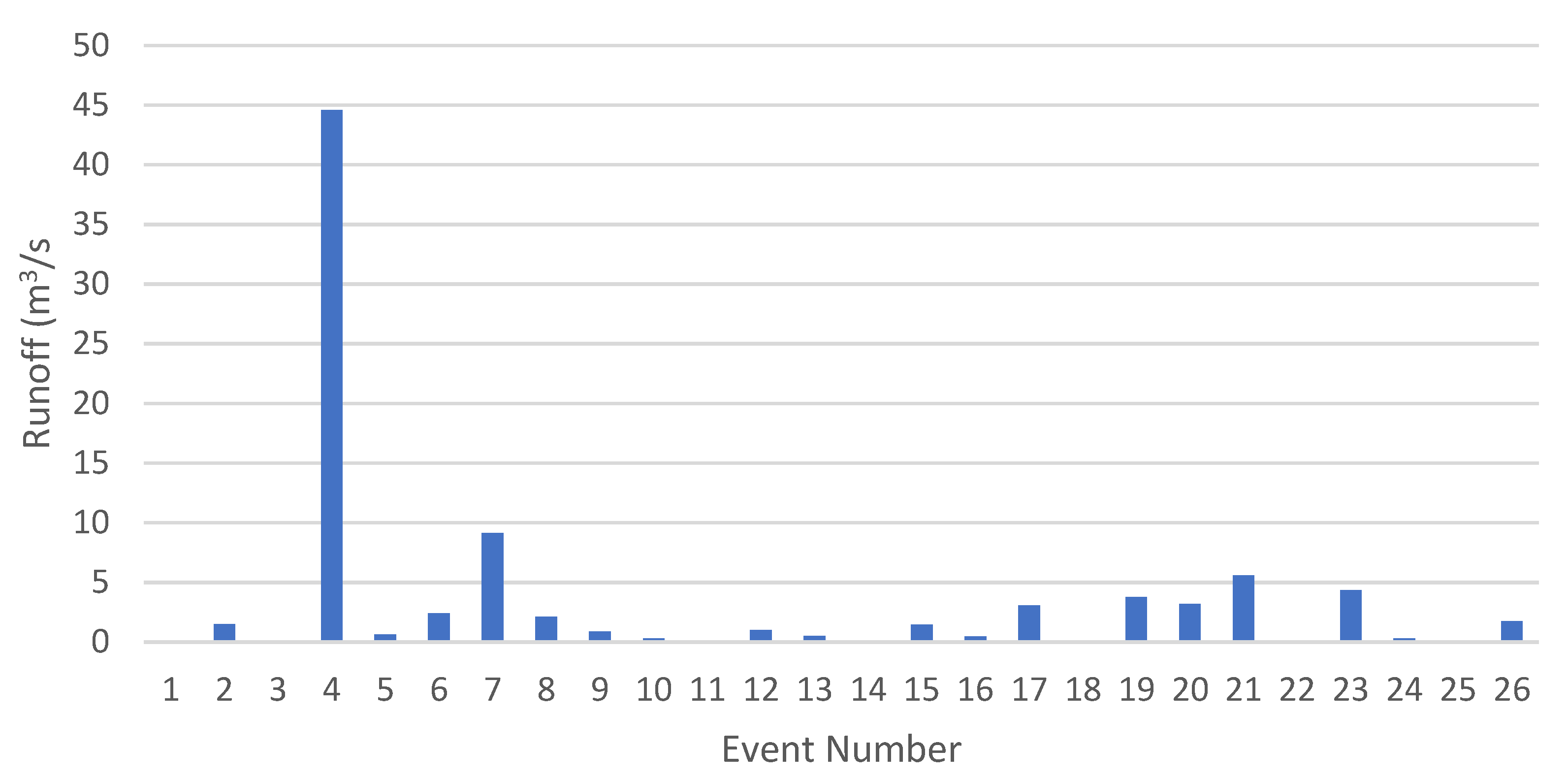
4.2. Rainfall-Runoff Modelling

Soil Conservation Service-Curve Number (SCS-CN) Method

The soil type within the catchment area was classified as Sand and Loamy Sand soil, based on the 8-point double ring infiltration field tests (

Table 5. Double ring infiltration in situ tests conducted to identify soil types.

Location ID	IR (mm/h)	Soil Type
A1	176.69	Sand
A2	59.48	Loamy sand
A3	157.50	Sand
A4	244.29	Sand
A5	124.68	Loamy sand
A6	379.49	Sand
A7	123.54	Loamy sand
A8	157.70	Sand

).

Soils are classified into four Hydrologic Soil Groups (HSGs): A, B, C, and D, based on soil infiltration rates (which is important for CN calculations). In accordance with the U.S. Department of Agriculture, Soil Group A is characterised by high infiltration rates, while the Soil Group B has moderate infiltration rates [49]. In addition, Groups C and D are characterised by low to very low infiltration rates, respectively. This classification was mainly based on the empirical experiments conducted by Cronshey (1986) of soil particle sizes. Consequently, the classification of the infiltration rate was identified as Group B, which is moderately low runoff potential. While the land use was described as an open space, the CN for Group B soil is 69 [50].

In addition, the impact of the station’s elevation above sea level on average rainfall was tested using the Pearson correlation, which gave a slightly significant value of around 0.59. However, the maximum retention after runoff begins at 4.49 mm, while initial abstraction is 0.90 mm. In addition, the antecedent soil moisture condition in the catchment fluctuates, based on several factors:

• Rainfall intensity and storm duration.
• Soil type and retention time.
• Temperature and other weather parameters.

As per Abushandi and Merkel (2013), there are three conditions of the Antecedent Moisture Condition (AMC) [30]:

• The soil moisture content is at welting point (soil profile is practically dry).
• Below saturation level: average condition occurred by some short rainfall storms but not long enough to create a runoff.
• The soil profile is practically saturated or super saturated from antecedent rainfall storms.

Generally, the behaviour of simulated runoff follows the observed runoff in the SCS method (Figure 9), while the performance showed some weaknesses when the observed runoff was less than 1 m³/s. In most cases, the simulated runoff using SCS tends to slightly underestimate the observed flood.

To simulate runoff using the SCS-CN method, the rainfall storms causing 26 runoff events were selected on a storm basis. The Nash–Sutcliffe Efficiency (NSE) was used to assess how perfectly the modelled SCS values compared with observed values. The NSE showed high performance at Hayl Al Adhah and Al Khan stations, with values of 0.92 and 0.94, respectively. The SCS results at Wadi Al Jizzi and Al Farfar stations showed a lower level of NSE, with values of 0.77 and 0.81, respectively. In reference to the station’s distance from the outlet, it is obvious that Wadi Al Jizzi and Al Farfar stations lie at greater distances from the outlet, which offers a chance for more water penetration and a higher level of uncertainty.

Based on the results, the Pearson correlation between the observed and simulated floods, using individual stations, was conducted. As expected, Wadi Al Jizzi and Al Farfar stations have lower values (

Table 6. Pearson correlation coefficient of simulated versus observed runoff rates for the four meteorological stations.

Simulated Runoff Using SCS	Observed Runoff at Sallan Station
Hayl Al Adhah	0.80
Al Khan	0.81
Al Farfar	0.59
Wadi Al Jizzi	0.56

).

The most sensitive parameter which may impact the values of SCS is the rainfall and its intensity. In addition, stream length influences the modelled values, coupled with curve number values. Approximately 50% of runoff occurs mainly in the months of February and March. The wet season starts in January to April with limited runoff in the summertime, due to tropical cyclonic storms from the Indian Ocean. The runoff event durations take place from a few minutes up to a couple of hours only. Nowadays, there are big efforts to produce raw data for further extreme hydrologic identification. Satellite-based precipitation products might be an alternative source of data to feed the Standard Precipitation Index (SPI) or any other drought indices. This will bridge the gap of data scarcity in arid areas (feeding lumped and distributed models) and allow possible drought and runoff risk analyses. Of course, some satellite data may produce misleading results, as the hydrologic algorithm simply does not reflect the variability of arid regions.

5. Conclusions

The application of the SPI and RAI showed the ability of both indices to identify extreme wet or dry levels. The SPI1 had a clear identification of dry or wet season, in connection to observed runoff records for the same periods. However, there was a consistent hydrologic distribution among the four stations, in terms of drought classification. In other words, distant stations from the outlet (closer to the mountains) have more extremely wet cases than the ones closer to the outlet. This phenomenon has been reflected by the higher performance of the Nash–Sutcliffe Efficiency for distant stations. Hence, rainfall intensity, catchment topography, and storm duration are important parameters in forming wet events. The SCS runoff simulation method could assess runoff events in arid catchments, taking into consideration that most of the simulated runoff is underestimated for all stations. However, this issue can be solved by re-adjusting the value using a simple linear regression model. The vital advantage of using the SCS runoff simulation method is the use of a different curve number value, based on the stations distributed in the catchment area, especially in regions with complex land cover types, and different stream lengths and soil types. In general, this research method can be utilised to estimate extreme events in arid areas if hydrological data are available. The performance of any model or indices on a different storm event could be different based on the recording interval and, therefore, the results will change accordingly. Sustainable development of the water sector during this difficult time is complicated, with a growing demand for using non-renewable water resources. Oman, as with many countries in the Middle East, is struggling to provide enough quality water for its domestic and agricultural needs. Therefore, this study is important for the understanding of hydrologic behaviour in arid catchments.

References

1. El Kenawy, A.M.; Al Buloshi, A.; Al-Awadhi, T.; Al Nasiri, N.; Navarro-Serrano, F.; Alhatrushi, S.; Robaa, S.M.; Domínguez-Castro, F.; McCabe, M.F.; Schuwerack, P.-M.; et al. Evidence for intensification of meteorological droughts in Oman over the past four decades. Atmos. Res. 2020, 246, 105126. [Google Scholar] [CrossRef]
2. Szalai, S.; Szinell, C.S. Comparison of two drought indices for drought monitoring in Hungary—A case study. In Drought and Drought Mitigation in Europe; Springer: Berlin/Heidelberg, Germany, 2000; pp. 161–166. [Google Scholar]
3. Conway, D. Extreme Hydrological Events: Precipitation, Floods and Droughts. J. Arid Environ. 1995, 29, 124–125. [Google Scholar] [CrossRef]
4. Dutta, R.; Maity, R. Time-varying network-based approach for capturing hydrological extremes under climate change with application on drought. J. Hydrol. 2021, 603, 126958. [Google Scholar] [CrossRef]
5. Kourgialas, N.N. Hydroclimatic impact on mediterranean tree crops area–Mapping hydrological extremes (drought/flood) prone parcels. J. Hydrol. 2021, 596, 125684. [Google Scholar] [CrossRef]
6. Adikari, K.E.; Shrestha, S.; Ratnayake, D.T.; Budhathoki, A.; Mohanasundaram, S.; Dailey, M.N. Evaluation of artificial intelligence models for flood and drought forecasting in arid and tropical regions. Environ. Model. Softw. 2021, 144, 105136. [Google Scholar] [CrossRef]
7. McKee, T.B.; Doesken, N.J.; Kleist, J. The relationship of drought frequency and duration to time scales. In Proceedings of the Proceedings of the 8th Conference on Applied Climatology, Anaheim, CA, USA, 17–22 January 1993; pp. 179–183. [Google Scholar]
8. Ali, M.; Deo, R.C.; Maraseni, T.; Downs, N.J. Improving SPI-derived drought forecasts incorporating synoptic-scale climate indices in multi-phase multivariate empirical mode decomposition model hybridized with simulated annealing and kernel ridge regression algorithms. J. Hydrol. 2019, 576, 164–184. [Google Scholar] [CrossRef]
9. Zhao, W.; Yan, T.; Peng, S.; Ding, M.; Lai, X. Drought and flood characteristics evolution in peninsular region of Shandong Province based on standardized precipitation index. In IOP Conference Series: Earth and Environmental Science; IOP Publishing: Bristol, UK, 2020; Volume 601, p. 12021. [Google Scholar]
10. Tsesmelis, D.E.; Vasilakou, C.G.; Kalogeropoulos, K.; Stathopoulos, N.; Alexandris, S.G.; Zervas, E.; Oikonomou, P.D.; Karavitis, C.A. Chapter 46—Drought assessment using the standardized precipitation index (SPI) in GIS environment in Greece. In Computers in Earth and Environmental Sciences; Pourghasemi, E.S., Ed.; Elsevier: Amsterdam, The Netherlands, 2022; pp. 619–633. ISBN 978-0-323-89861-4. [Google Scholar]
11. Łabędzki, L. Estimation of local drought frequency in central Poland using the standardized precipitation index SPI. Irrig. Drain. J. Int. Comm. Irrig. Drain. 2007, 56, 67–77. [Google Scholar] [CrossRef]
12. Zhai, J.; Su, B.; Krysanova, V.; Vetter, T.; Gao, C.; Jiang, T. Spatial variation and trends in PDSI and SPI indices and their relation to streamflow in 10 large regions of China. J. Clim. 2010, 23, 649–663. [Google Scholar] [CrossRef]
13. Tufaner, F.; Özbeyaz, A. Estimation and easy calculation of the Palmer Drought Severity Index from the meteorological data by using the advanced machine learning algorithms. Environ. Monit. Assess. 2020, 192, 1–14. [Google Scholar] [CrossRef]
14. Abushandi, E.; Merkel, B. Rainfall estimation over the Wadi Dhuliel arid catchment, Jordan from GSMaP_MVK+. Hydrol. Earth Syst. Sci. Discuss. 2011, 8, 1665–1704. [Google Scholar]
15. Abushandi, E. Flash flood simulation for Tabuk City catchment, Saudi Arabia. Arab. J. Geosci. 2016, 9, 1–10. [Google Scholar] [CrossRef]
16. Shadeed, S.; Almasri, M. Application of GIS-based SCS-CN method in West Bank catchments, Palestine. Water Sci. Eng. 2010, 3, 1–13. [Google Scholar]
17. Alzghoul, M.; Al-husban, Y. Estimation of Runoff by applying SCS Curve Number Method, in a complex arid area; Wadi Al-Mujib watershed; Study case. Dirasat Hum. Soc. Sci. 2021, 48. Available online: https://archives.ju.edu.jo/index.php/hum/article/view/104919 (accessed on 22 May 2022).
18. El-Hames, A.S. An empirical method for peak discharge prediction in ungauged arid and semi-arid region catchments based on morphological parameters and SCS curve number. J. Hydrol. 2012, 456, 94–100. [Google Scholar] [CrossRef]
19. Al-Ghobari, H.; Dewidar, A.; Alataway, A. Estimation of Surface Water Runoff for a Semi-Arid Area Using RS and GIS-Based SCS-CN Method. Water 2020, 12, 1924. [Google Scholar] [CrossRef]
20. Braud, I.; Borga, M.; Gourley, J.; Hurlimann, M.; Zappa, M.; Gallart, F. Flash floods, hydro-geomorphic response and risk management. J. Hydrol. 2016, 541, 1–5. [Google Scholar] [CrossRef] [Green Version]
21. Karagiorgos, K.; Thaler, T.; Heiser, M.; Hübl, J.; Fuchs, S. Integrated flash flood vulnerability assessment: Insights from East Attica, Greece. J. Hydrol. 2016, 541, 553–562. [Google Scholar] [CrossRef]
22. Mahmood, M.I.; Elagib, N.A.; Horn, F.; Saad, S.A.G. Lessons learned from Khartoum flash flood impacts: An integrated assessment. Sci. Total Environ. 2017, 601–602, 1031–1045. [Google Scholar] [CrossRef]
23. Abushandi, E.; Al Sarihi, M. Flash flood inundation assessment for an arid catchment, case study at Wadi Al Jizzi, Oman. Water Pract. Technol. 2022, 17, 1155–1168. [Google Scholar] [CrossRef]
24. Al Ruheili, A.; Dahm, R.; Radke, J. Wadi flood impact assessment of the 2002 cyclonic storm in Dhofar, Oman under present and future sea level conditions. J. Arid Environ. 2019, 165, 73–80. [Google Scholar] [CrossRef]
25. Niyazi, B.A.; Masoud, M.H.; Ahmed, M.; Basahi, J.M.; Rashed, M.A. Runoff assessment and modeling in arid regions by integration of watershed and hydrologic models with GIS techniques. J. Afr. Earth Sci. 2020, 172, 103966. [Google Scholar] [CrossRef]
26. Saber, M.; Hamaguchi, T.; Kojiri, T.; Tanaka, K.; Sumi, T. A physically based distributed hydrological model of wadi system to simulate flash floods in arid regions. Arab. J. Geosci. 2015, 8, 143–160. [Google Scholar] [CrossRef]
27. El Alfy, M. Assessing the impact of arid area urbanization on flash floods using GIS, remote sensing, and HEC-HMS rainfall–runoff modeling. Hydrol. Res. 2016, 47, 1142–1160. [Google Scholar] [CrossRef]
28. Jodar-Abellan, A.; Valdes-Abellan, J.; Pla, C.; Gomariz-Castillo, F. Impact of land use changes on flash flood prediction using a sub-daily SWAT model in five Mediterranean ungauged watersheds (SE Spain). Sci. Total Environ. 2019, 657, 1578–1591. [Google Scholar] [CrossRef] [PubMed]
29. Aghabeigi, N.; Esmali, O.A.; Mostafazadeh, R.; Golshan, M. The Effects of Climate Change on Runoff Using IHACRES Hydrologic Model in Some of Watersheds, Ardabil Province. Irrig. Water Eng. 2020, 10, 178–189. [Google Scholar]
30. Abushandi, E.; Merkel, B. Modelling rainfall runoff relations using HEC-HMS and IHACRES for a single rain event in an arid region of Jordan. Water Resour. Manag. 2013, 27, 2391–2409. [Google Scholar] [CrossRef]
31. Siebert, S.; Nagieb, M.; Buerkert, A. Climate and irrigation water use of a mountain oasis in northern Oman. Agric. Water Manag. 2007, 89, 1–14. [Google Scholar] [CrossRef]
32. Searle, M.P. Preserving Oman’s geological heritage: Proposal for establishment of World Heritage Sites, National GeoParks and Sites of Special Scientific Interest (SSSI). Geol. Soc. London, Spec. Publ. 2014, 392, 9–44. [Google Scholar] [CrossRef]
33. Al-Kindi, R.S. Assessment of Groundwater Recharge from the Dam of Wadi Al-Jizzi, Sultanate of Oman; United Arab Emirates University: Al Ain, United Arab Emirates, 2014. [Google Scholar]
34. Al Maqbali, N. Risk Assessment of Dams; University of Adelaide: Adelaide, Australia, 1999. [Google Scholar]
35. Abushandi, E. Flood Water Management in Arid Regions, Case Studies: Wadi Al Jizzi, Oman, Wadi Abu Nsheifah, Saudi Arabia, and Wadi Dhuleil, Jordan. In Recent Advances in Environmental Science from the Euro-Mediterranean and Surrounding Regions; Kallel, A., Ksibi, M., Ben Dhia, H., Khélifi, N., Eds.; Springer International Publishing: Cham, Switzerland, 2018; pp. 1813–1814. [Google Scholar]
36. Costa, J.A.; Rodrigues, G.P. Space-time distribution of rainfall anomaly index (RAI) for the Salgado Basin, Ceará State-Brazil. Ciência e Nat. 2017, 39, 627–634. [Google Scholar] [CrossRef] [Green Version]
37. Zhao, H.; Gao, G.; An, W.; Zou, X.; Li, H.; Hou, M. Timescale differences between SC-PDSI and SPEI for drought monitoring in China. Phys. Chem. Earth Parts A/B/C 2017, 102, 48–58. [Google Scholar] [CrossRef]
38. Wang, S.; Najafi, M.R.; Cannon, A.J.; Khan, A.A. Uncertainties in Riverine and Coastal Flood Impacts under Climate Change. Water 2021, 13, 1774. [Google Scholar] [CrossRef]
39. Verma, S.; Singh, P.K.; Mishra, S.K.; Singh, V.P.; Singh, V.; Singh, A. Activation soil moisture accounting (ASMA) for runoff estimation using soil conservation service curve number (SCS-CN) method. J. Hydrol. 2020, 589, 125114. [Google Scholar] [CrossRef]
40. Liu, J.; Yuan, D.; Zhang, L.; Zou, X.; Song, X. Comparison of Three Statistical Downscaling Methods and Ensemble Downscaling Method Based on Bayesian Model Averaging in Upper Hanjiang River Basin, China. Adv. Meteorol. 2016, 2016, 7463963. [Google Scholar] [CrossRef] [Green Version]
41. Shadeed, S. Spatio-temporal drought analysis in arid and semi-arid regions: A case study from Palestine. Arab. J. Sci. Eng. 2013, 38, 2303–2313. [Google Scholar] [CrossRef]
42. Sienz, F.; Bothe, O.; Fraedrich, K. Monitoring and quantifying future climate projections of dryness and wetness extremes: SPI bias. Hydrol. Earth Syst. Sci. 2012, 16, 2143–2157. [Google Scholar] [CrossRef] [Green Version]
43. Conradie, W.S.; Wolski, P.; Hewitson, B.C. Spatial heterogeneity of 2015–2017 drought intensity in South Africa’s winter rainfall zone. Adv. Stat. Clim. Meteorol. Oceanogr. 2022, 8, 63–81. [Google Scholar] [CrossRef]
44. Glad, P.A. Meteorological and Hydrological Conditions Leading to Severe Regional Drought in Malawi. Master’s Thesis, University of Oslo, Oslo, Norway, 2010. [Google Scholar]
45. Mahmoudi, P.; Ghaemi, A.; Rigi, A.; Amir Jahanshahi, S.M. Recommendations for modifying the Standardized Precipitation Index (SPI) for drought monitoring in arid and semi-arid regions. Water Resour. Manag. 2021, 35, 3253–3275. [Google Scholar] [CrossRef]
46. Wu, H.; Svoboda, M.D.; Hayes, M.J.; Wilhite, D.A.; Wen, F. Appropriate application of the standardized precipitation index in arid locations and dry seasons. Int. J. Climatol. A J. R. Meteorol. Soc. 2007, 27, 65–79. [Google Scholar] [CrossRef]
47. Musonda, B.; Jing, Y.; Iyakaremye, V.; Ojara, M. Analysis of Long-Term Variations of Drought Characteristics Using Standardized Precipitation Index over Zambia. Atmosphere 2020, 11, 1268. [Google Scholar] [CrossRef]
48. Mehr, A.D.; Vaheddoost, B. Identification of the trends associated with the SPI and SPEI indices across Ankara, Turkey. Theor. Appl. Climatol. 2020, 139, 1531–1542. [Google Scholar] [CrossRef]
49. U.S. Department of Agriculture. Hydrologic Soil Groups. In National Engineering Handbook. Part 630 Hydrology, Chapter 7; U.S. Department of Agriculture: Washington, DC, USA, 2009; pp. 1–13. [Google Scholar]
50. Cronshey, R. Urban Hydrology for Small Watersheds; No. 55; US Department of Agriculture, Soil Conservation Service, Engineering Division: Washington, DC, USA, 1986.
Figure 1. Location and natural drainage network of the Wadi Al Jizzi catchment.
Sustainability 14 14028 g001
Figure 2. The volcanic stones in Wadi Al-Jizzi.
Sustainability 14 14028 g002
Figure 3. The mean of monthly climatological rainfall distribution for the selected stations.
Sustainability 14 14028 g003
Figure 4. Runoff records from Sallan station for the period between 1987 and 2007.
Sustainability 14 14028 g004
Figure 5. Infiltration boreholes and station locations within the catchment area.
Sustainability 14 14028 g005
Figure 6. The SPI1 classification frequencies and percentages at the four selected rainfall stations.
Sustainability 14 14028 g006
Figure 7. The RAI classification frequencies and percentages at the four selected rainfall stations.
Sustainability 14 14028 g007
Figure 8. SPI 3-month drought records for the wet season.
Sustainability 14 14028 g008
Figure 9. Wadi Al Jizzi catchment observed vs. SCS simulated runoff (26 runoff records), where: (a) is Al Farfar Station; (b) is Al Khan Station; (c) is Hayl Al Adhah Station; and (d) is Wadi Al Jizzi Station.
Sustainability 14 14028 g009