The Spatial Disequilibrium and Dynamic Evolution of the Net Agriculture Carbon Effect in China

Abstract

Considering the comparative perspective of the net agricultural carbon effect in China’s three major functional grain production areas, the Dagum Gini coefficient, kernel density estimation and Markov chain analysis are used to investigate the spatial disequilibrium and dynamic evolution characteristics of the net agricultural carbon effect in China from 2000 to 2019. The results show that the overall net agricultural carbon sink in China is on a fluctuating upward trend, and the net agricultural carbon sink in the main production areas is higher than that in main marketing areas and balanced production and marketing areas. There are obvious differences in the net agricultural carbon sink between different areas, and the differences are expanding; inter-regional differences are the most significant, with the contribution of intra-regional differences second and the contribution of intensity of transvariation the least. The kernel density curve shows that the absolute differences are increasing and that there are gradients and multipolar differentiation within the area. The Markov transfer matrix reflects that the net agricultural carbon effect in China is highly volatile and has a strong internal mobility. The probability of upward shift in an area increases when it is adjacent to a high-level area, and the net carbon effect of agriculture in high-level areas has a strong stability. Based on this, each area should build on its own comparative advantages and explore targeted pathways to reducing emissions and increasing sinks in agriculture while strengthening inter-regional communication and cooperation. It is necessary to build a synergistic mechanism to enhance the net carbon effect of agriculture, which will ultimately help to achieve the “double carbon” target.

1. Introduction

Climate change is a global problem facing mankind. The rapid increase in carbon emissions has intensified the greenhouse effect. Glacier melting, frequent disasters, and rising temperatures are affecting all aspects of human life. As the world’s second largest economy and the largest developing country, China has actively joined the global climate governance initiative, demonstrating its responsible and committed role as a major power. In September 2020, China made it clear that it would adopt stronger policies and measures to achieve peak carbon by 2030 and carbon neutrality by 2060, or the “double carbon” target. In December 2020, China further stated at the Climate Ambition Summit that by 2030, China’s CO₂ emissions per unit of GDP would be more than 65% lower than in 2005. The report of the 20th National Congress of the CPC clearly mentioned that China should actively and steadily promote carbon peak and carbon neutrality to deal with the global governance of climate change. However, at present, the control of carbon emissions is mainly focused on industrial production, which is considered to be the most important source of greenhouse gas emissions but has little to do with agriculture [1]. In fact, according to the fifth IPCC assessment report, agricultural production has become the second largest emission source of greenhouse gases in the world. According to data released by the Food and Agriculture Organization of the United Nations (FAO), agricultural production releases more than 30% of global CO₂ emissions, and as a special production sector, agriculture also has carbon sequestration and sinking properties, but agro-ecosystems can also offset 80% of the CO₂ emissions caused by agriculture. Therefore, under the double carbon objective, agriculture must reduce emissions, sequester carbon to increase sinks and serve carbon neutrality. At the same time, an important function of agriculture is ensuring the national food security. Each functional food production area has different resource endowments, functional plans and economic structures. Distinctive geographical types of agriculture have been formed, generating different amounts of carbon sinks, sources and net carbon sinks [2]. This poses a serious challenge to the coordinated development of low-carbon agriculture. Many countries have made arrangements for carbon emission and carbon reduction, and many scholars have explored how to achieve carbon neutrality from the perspectives of energy utilization, financial support, industrial structure and consumption habits [3,4]. In view of this, considering the scientific evaluation of the net carbon effect of Chinese agriculture, this paper accurately grasps its spatial disequilibrium characteristics and dynamic evolution trends. It is of great practical significance to actively and steadily promote the realization of the double carbon target.

2. Literature Review

Promoting the transition from high carbon to low carbon should be started from the two aspects of carbon sink and carbon source [5]. On the one hand, carbon sinks refer to carbon uptake and are regarded as ecological welfare [6,7]. Piao used atmospheric inversions and terrestrial carbon models and analysed recent changes in the net land carbon sink (NLS) and its driving factors [8]. Wang found that vegetation greenness increased significantly over time, which supported the timing of and increase in terrestrial carbon sinks in afforestation areas [9]. Wu established a stochastic multi-objective nonlinear programming model under the framework of socioeconomic ecology that can consider the carbon sink function of farmland vegetation [10]. Zhu compiled a complete set of forest inventory data from North America north of Mexico to understand the fate of forest biomass as a carbon sink and to predict its potential in mitigating climate change [11]. Piao reviewed the assessments of China’s terrestrial ecosystem carbon sink, with focus on the principles, frameworks and methods of terrestrial ecosystem carbon sink estimates, as well as the recent progress and existing problems [12]. Singh believed that the world’s soil has the largest organic carbon storage in the terrestrial ecosystem. By determining a series of traditional and emerging agricultural management practices in farmland, Singh emphasized that knowledge and mechanisms may increase organic carbon storage [13]. Sha proposed an integrated method of assessing how much more carbon can be sequestered by vegetation if optimal land management practices are implemented. The proposed method combines remotely sensed time series of net primary productivity datasets, segmented landscape–vegetation–soil zones and distance-constrained zonal analysis [14]. Lorenz focused on scientific understanding of SiC and organic carbon sequestration in agro-ecosystems [15]. Sun calculated the economic value of mariculture carbon sinks based on carbon tax law and afforestation law [16]. On the other hand, carbon sources refer to carbon emissions and are seen as undesirable outputs [17,18]. Among them, some scholars discussed agricultural carbon emissions from a single-dimensional perspective, such as planting [17,18,19,20], livestock and poultry breeding [19,20,21,22,23,24,25] and fishery production [26,27,28,29]. Some scholars integrated multidimensional carbon sources for investigation. Johnson argued that ACESs were mainly derived from intestinal fermentation in livestock, manure management, rice growth and the arbitrary disposal of agricultural waste [30]. Huang and Zhang et al. estimated the amount and intensity of agricultural carbon emissions in China from five carbon sources, agricultural materials, rice planting, soil N₂O, livestock and poultry farming and straw burning and analysed their spatial and temporal characteristics [31,32]. Xiong believed that agricultural greenhouse gas emissions mainly come from the use of agricultural land and livestock farming [33,34]. Ghosh considered carbon emissions from three main sectors of agriculture, namely agriculture, fisheries and dairy [35]. Cui analysed the regional differences in and temporal and spatial dynamic evolution of planting industry carbon emission intensity considering the carbon sink effect and found that China’s planting industry carbon emission intensity showed a significant disequilibrium distribution when considering the carbon sink effect [36]. Shan believed that in addition to agricultural production materials and livestock and poultry breeding, agricultural carbon emissions in Hubei Province should also include rural living energy consumption and household waste disposal in the calculation scope [37]. The measurement of agricultural carbon emissions in the above literature mostly adopts the carbon emission coefficient method.

After completing the analysis and calculation of the agricultural carbon sink and carbon source index system, Popp discussed how to implement carbon offsets in agriculture [38]. In addition, many scholars have studied the distribution characteristics of agricultural net carbon. Tian measured the net carbon sink of the planting industry and found that the regional differences were obvious [39]. Chen used ArcGIS visualization to analyze the change law of the spatial pattern of China’s county-level agricultural net carbon sink and found that the regional gap is constantly narrowing [40]. Xiong calculated agricultural carbon emissions and carbon sinks using the data in Hotan Prefecture and found that the net carbon sink in Hotan Prefecture showed a steady growth trend during the sample period [41]. Pei analysed the spatial and temporal dynamics of carbon emissions and carbon sinks in Guangdong Province, southern China, in which the carbon sinks only calculated forest land and grassland and did not consider farmland [42]. Li used DEA to calculate the agricultural net carbon sink efficiency in China’s provinces and used kernel density estimation to analyze the spatial and temporal dynamic evolution process and found that there is an obvious regional disequilibrium phenomenon in China’s agricultural net carbon sink efficiency [43]. Weng used methods such as standard deviation ellipse to find that the net carbon sink in farmland ecosystems in Jiangsu Province presents a spatial distribution pattern of northwest–southeast [44].

The abovementioned literature has laid a solid foundation for the development of this paper, but there are also shortcomings. (1) The existing literature on the net carbon effect of agriculture is mainly from the perspective of geographical location, and there is a lack of studies that take the net carbon effect of agriculture in food production functional areas as the object of investigation. (2) The existing literature on carbon sink measurement is mostly focused on the crop level, while there are fewer studies that include forest land and grassland in the carbon sink measurement system. (3) The existing literature only gives a brief description of the current situation of agricultural net carbon effect through descriptive statistical analysis and does not deeply discuss the evolution trend in agricultural net carbon effect from a spatial perspective. Based on this, this paper will expand and deepen in the following three aspects: (1) In view of the scale of functional areas of food production, the three main functional areas of food production, main marketing areas and balanced production and marketing areas are analysed for the development trends in their agricultural net carbon effects. (2) A checklist of agricultural inputs, paddy methane, agricultural land use, livestock breeding and biological carbon sequestration is constructed in which crops, woodlands and grasslands are included in the measurement of biological carbon sequestration to accurately measure the net carbon sink of Chinese agriculture. (3) With the help of the Dagum Gini coefficient, the spatial disequilibrium characteristics and dynamic evolution of China’s agricultural net carbon effect are investigated comprehensively.

The remainder of this paper is organized as follows. Section 3 introduce the research methods and data processing. In Section 4, the spatial disequilibrium characteristics of the net agricultural carbon effect are measured and analysed using the Gini coefficient, and in Section 5, the dynamic evolution of the net agriculture carbon effect is measured using the kernel density and Markov chain. The conclusions and implications of the paper are presented in Section 4.

3. Model Construction and Data Measurement

3.1. Model Construction

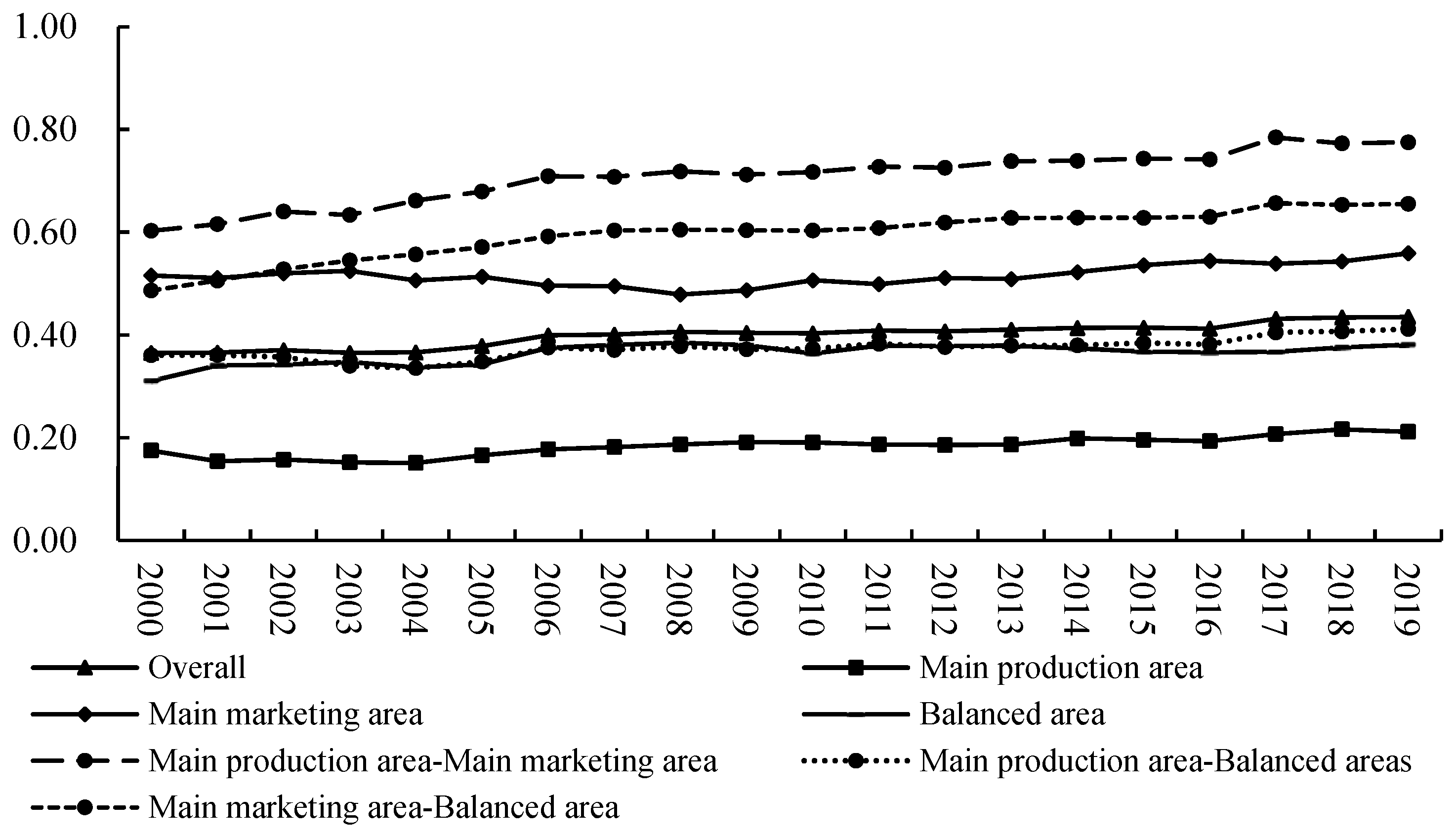
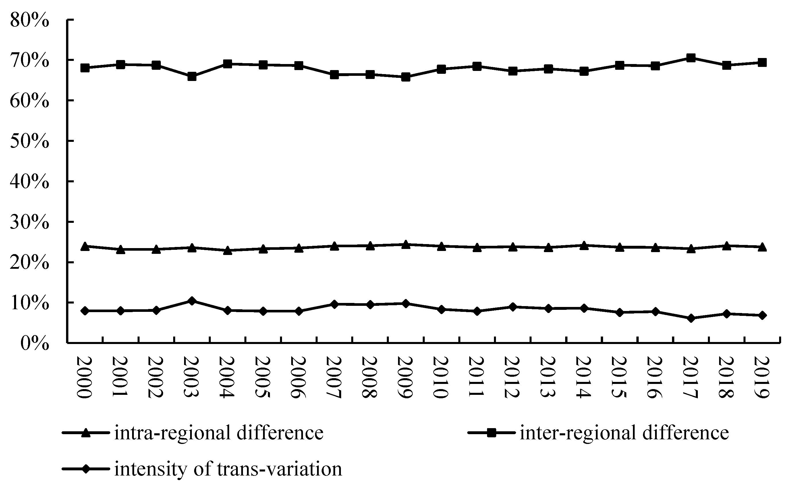
3.1.1. Dagum Gini Coefficient and Its Decomposition Method

Dagum proposed a decomposition method based on subsamples. According to this method, the Gini coefficient can be decomposed into three components: there are the contributions by the intra-regional differences $G_w$, inter-regional differences $G_{nb}$ and intensity of transvariation $G_t$ [45]. This method fully considers the distribution status of subsamples. It identifies the sources of the regional differences and effectively solves the problem of the overlaps between the sample data. In particular, the overall Gini coefficient $G$, the intra-regional Gini coefficient $Gjj$ and the inter-regional Gini coefficient $Gjh$ are calculated as follows:

$$G=\frac{{\displaystyle \sum _{j=1}^k{\displaystyle \sum _{h=1}^k{\displaystyle \sum _{i=1}^{n_j}{\displaystyle \sum _{r=1}^{n_h}\left|Y_{ji}-Y_{hr}\right|}}}}}{2n^2\overline{Y}}$$

(1)

$$G_{jj}=\frac{\frac{1}{2\overline{y_j}}{\displaystyle \sum _{i=1}^{n_j}{\displaystyle \sum _{r=1}^{n_h}\left|Y_{ji}-Y_{hr}\right|}}}{n_j{}^2}$$

(2)

$$G_{jh}=\frac{{\displaystyle \sum _{i=1}^{n_j}{\displaystyle \sum _{r=1}^{n_h}\left|Y_{ji}-Y_{hr}\right|}}}{n_j{n}_h^{}(\overline{Y_j}+\overline{Y_h})}$$

(3)

In Formulas (1)–(3), $j$ and $h$ represent different areas, $k$ is the number of areas, $n$ is the number of provinces in the sample, $n_j(n_h)$ is the number of provinces in area $j(h)$, $Y_{ji}(Y_{hr})$ is the net agricultural carbon sink of province $i(r)$ in area $j(h)$ and $\overline{Y}$ is the overall average of net agricultural carbon sinks in China. The overall Gini coefficient $G$ is further decomposed into intra-regional variance contribution $G_w$, inter-regional variance contribution $G_{nb}$ and super-variance density contribution $G_t$, and all satisfy $G=G_w+G_{nb}+G_t$, which are calculated as follows, respectively:

$$G_w={\displaystyle \sum _{j=1}^k{G}_{jj}{P}_j{S}_j}$$

(4)

$$G_{nb}={\displaystyle \sum _{j=2}^k{\displaystyle \sum _{h=1}^{j-1}{G}_{jh}(P_j{S}_h+P_h{S}_j)D_{jh}}}$$

(5)

$$G_t={\displaystyle \sum _{j=2}^k{\displaystyle \sum _{h=1}^{j-1}{G}_{jh}(P_j{S}_h+P_h{S}_j)(1-D_{jh})}}$$

(6)

$$D_{jh}=\frac{d_{jh}-P_{jh}}{d_{jh}+P_{jh}}$$

(7)

$$d_{jh}={\displaystyle {\int }_0^{\infty }d{F}_j(y){\displaystyle {\int }_0^Y(Y-x)d{F}_h(x)}}$$

(8)

$$P_{jh}={\displaystyle {\int }_0^{\infty }d{F}_h(y){\displaystyle {\int }_0^Y(Y-x)d{F}_j(y)}}$$

(9)

In Formula (4), $P_j=n_j/n$ is the number of provinces in the $n$ area as a percentage of the country, and $S_j=n_j\overline{Y_j}/n\overline{Y},j=1,2,\cdots ,k$. $D_{jh}$ in Formulas (5) and (6) are the interactions of the net agricultural carbon effect between different areas. In Formulas (7) and (8), $d_{jh}$ and $P_{jh}$ denote the mathematical expectation of the sum of all sample values of $y_{ji}>y_{hr}$ and $y_{ji}<y_{hr}$ in areas $j$ and $h$, respectively. $F_j(F_h)$ is the cumulative density distribution function for area $j(h)$ in Formula (9).

3.1.2. Kernel Density Estimation Method

Kernel density estimation is a nonparametric estimation method that uses continuous density function curves to describe the distribution patterns of random variables. It is commonly used to analyse the dynamic characteristics of the spatiotemporal distribution of random variables [46]. The kernel density estimator is given by the following Formula (10). $X_i$ represents the net agricultural carbon sink in each province, $\overline{x}$ is the mean net agricultural carbon sink, $N$ is the number of observations in the evaluation area, $h$ is the bandwidth and $K(•)$ is the kernel density function. Based on the existing literature, this paper uses the Gauss kernel function for estimation, and the kernel function is Formula (11).

$$f(x)=\frac{1}{Nh}{\displaystyle \sum _{i=1}^{N}K(\frac{X_i-\overline{x}}{h})}$$

(10)

$$K(x)=\frac{1}{\sqrt{2\pi }}\exp \left(\frac{-x^2}{2}\right)$$

(11)

3.1.3. Markov Chain Analysis

(1) Traditional Markov chain analysis. The traditional Markov chain is an analysis method that reflects the probability of a random variable moving to a low or high level over time in the form of a transfer probability matrix and predicts the liquidity and evolution trend within the system. In the analysis, $t$ corresponds to each period, and the finite states correspond to the number of states of the random variable. The net agricultural carbon sink is divided into four levels: low, medium-low, medium-high and high. In turn, a transfer probability matrix (as in

Table 1. Markov chain state transfer probability matrix (N = 4).

ti/ti+1	1	2	3	4
1	P11	P12	P13	P14
2	P21	P22	P23	P24
3	P31	P32	P33	P34
4	P41	P42	P43	P44

) is obtained, so that the state transfer probability matrix can reveal the state evolution trend in the net carbon effect of agriculture in China.

(2) Spatial Markov chain analysis. In order to examine the influence of spatial factors on the probability of state transfer, the spatial lag was incorporated into the traditional Markov chain analysis [47]. The spatial weight matrix (spatial adjacency matrix) is first set, and then the traditional transfer probability matrix is decomposed into four transfer conditional probability matrices. The spatial transfer probabilities of net agricultural carbon sinks from periods to low levels or to high levels are considered under the influence of different levels of neighbours (low, medium-low, medium-high and high;

Table 2. Spatial Markov chain state transfer probability matrix (N = 4).

Lag Type	ti/ti+1	1	2	3	4
1	1	P11	P12	P13	P14
	2	P21	P22	P23	P24
	3	P31	P32	P33	P34
	4	P41	P42	P43	P44
2	1	P11	P12	P13	P14
	2	P21	P22	P23	P24
	3	P31	P32	P33	P34
	4	P41	P42	P43	P44
3	1	P11	P12	P13	P14
	2	P21	P22	P23	P24
	3	P31	P32	P33	P34
	4	P41	P42	P43	P44
4	1	P11	P12	P13	P14
	2	P21	P22	P23	P24
	3	P31	P32	P33	P34
	4	P41	P42	P43	P44

), thus revealing the influence of spatial factors on the transfer trends in net agricultural carbon effects.

3.2. Data Measurement

Agriculture, as a special production sector, shows the dual attributes of carbon sink and carbon source in its participation in the carbon cycle. While considering the dual attributes, the net carbon effect of agriculture in this study is essentially the net carbon sink of agriculture. In other words, the net agricultural carbon sink is the difference between the agricultural carbon sink and the agricultural carbon source, where the system and methods for measuring the agricultural carbon sink and the agricultural carbon source are as follows.

Agricultural carbon sink is the amount of organic carbon absorbed and fixed by crops, forest trees and grasslands through photosynthesis during the growth cycle. The agricultural carbon sink ($C_a$) is equal to the sum of the crop carbon sink ($C_{a1}$) and the woodland and grassland carbon sink ($C_{a2}$). That is, $C_a=(C_{a1}+C_{a2})$. The specific calculations of crop, forest and grassland carbon sinks are shown in Formulas (12) and (13). In Formula (12), $C_{a1}$ is the crop carbon sink, $k$ is the number of crop species, $C_{ai}$ is the carbon sink of the crop $i$, $L_i$ is the amount of carbon required to be absorbed by the crop $i$ to synthesise a unit of organic matter, $W_i$ is the average water content, $Y_i$ is the economic yield and $H_i$ is the economic coefficient. The carbon sinks of crops are mainly calculated for 15 species such as rice, wheat, maize, beans, potatoes and sugar beet. The carbon uptake coefficient, water content and economic coefficient of crops were selected with reference to the study by Tian [48]. In Formula (13), $C_{a2}$ is the carbon sink of woodland and grassland, $m$ is the woodland or grassland ($m=1,2$), $Sm$ is the area of the land type $m$ and ${\alpha }_m$ is the carbon sequestration coefficient of the land type $m$. Referring to the study by Zhou, the carbon sequestration coefficients of woodland and grassland were 3.81 t/hm² and 0.91 t/hm², respectively [49].

$$C_{a1}={\displaystyle \sum _i^k{C}_a{}_i}={\displaystyle \sum _i^k{L}_i\times (1-W_i)\times }\frac{Y_i}{H_i}$$

(12)

$$C_{a2}={\displaystyle \sum _{i=1}^m{S}_m\times }{\alpha }_m$$

(13)

Agricultural carbon sources are the greenhouse gases released into the atmosphere from agricultural production activities. Four categories of carbon sources were selected: agricultural inputs, methane from rice fields, agricultural land use and livestock farming. Among them, agricultural inputs include fertilizers, pesticides, agricultural films, agricultural diesel and irrigation. The methane emissions from rice fields and nitrous oxide emissions from crop cultivation can damage the soil surface layer. Greenhouse gas emissions of methane and nitrous oxide are generated from the gastrointestinal fermentation of livestock and poultry during livestock farming and from manure emissions. Livestock species include cattle, horses, pigs, sheep and poultry, and their emission coefficients refer to the study by Tian [48]. In Formula (14), $C_e$ is the total amount of agricultural carbon sources. $C_i$ is the amount of carbon sources generated by the consumption of sources $i$. ${\xi }_i$ is the emission coefficient for a particular type of carbon source. $T_i$ is the total amount of a particular type of carbon source. To facilitate aggregation and analysis, CH₄ and N₂O emissions were converted to standard carbon, with 1 kg CH₄ and 1 kg N₂O equivalent to 6.8182 kg C and 81.2727 kg C, respectively. The data used in this study include 31 provincial administrative areas in China. In view of the availability of data, Hong Kong, Macao and Taiwan were not included in this study. The data were obtained from the China Statistical Yearbook, China Rural Statistical Yearbook and China Agricultural Yearbook in previous years. Individual missing data were linearly interpolated using values from neighbouring years.

$$C_e={\displaystyle \sum C_{ei}={\displaystyle \sum {\xi }_i{T}_i}}$$

(14)

4. Typical Factual Analysis of Net Carbon Effect of Agriculture

4.1. Analysis of the Measurement of Net Carbon Sinks in Agriculture

Table 3. Estimated results of some years of agricultural net carbon sinks in China’s provinces and three major grain production areas.

Province	2000	2002	2004	2006	2008	2010	2012	2014	2016	2018	2019
Hebei	2.2836	2.2651	2.2974	2.6946	2.8029	2.9194	3.1741	3.2544	3.4441	3.6376	3.7428
Inner Mongolia	3.3065	3.4664	3.5070	3.7941	4.0887	4.2974	4.6310	4.9232	4.9848	5.8091	5.9421
Liaoning	1.0362	1.4330	1.5796	1.6730	1.7039	1.6407	1.9764	1.6184	1.9727	2.1501	2.4353
Jilin	1.7736	2.3895	2.5812	2.8022	2.8925	2.8404	3.3107	3.4789	3.6235	3.6097	3.8628
Heilongjiang	3.0953	3.4792	3.4405	4.1722	4.4984	5.1252	5.7149	6.1569	5.9596	7.4000	7.5056
Jiangsu	2.4231	2.3628	2.4111	2.5732	2.6297	2.7064	2.8550	3.0031	2.9510	3.1441	3.2906
Anhui	2.2080	2.4386	2.5076	2.7621	2.8637	2.8909	3.0526	3.1964	3.1214	3.6214	3.7091
Jiangxi	1.6508	1.6164	1.6784	1.8579	1.9135	1.9355	2.0483	2.1024	2.0877	2.1835	2.2107
Shandong	3.6536	3.1530	3.5532	4.1168	4.4286	4.2783	4.4650	4.5589	4.6801	5.3158	5.4187
Henan	3.8275	3.9740	4.0135	5.1348	5.4572	5.4088	5.5576	5.6529	5.8887	6.6996	6.873
Hubei	2.2801	2.0653	2.2029	2.2085	2.2932	2.4061	2.5410	2.7081	2.6291	2.8534	2.8675
Hunan	2.4262	2.1966	2.2824	2.3811	2.4528	2.5954	2.7428	2.7486	2.7637	2.8575	2.941
Sichuan	3.2586	3.0725	3.1608	2.9857	3.2271	3.3890	3.4797	3.5721	3.6966	3.9967	4.1378
Average value of main production areas	1.9513	1.9863	2.0571	2.2394	2.3850	2.4313	2.6081	2.6759	2.7052	2.9557	3.0405
Beijing	0.1336	0.0775	0.0762	0.1252	0.1394	0.1306	0.1222	0.0830	0.0753	0.0690	0.0641
Tianjin	0.1163	0.1425	0.1450	0.1479	0.1428	0.1482	0.1491	0.1545	0.1703	0.1891	0.2074
Shanghai	0.1264	0.0922	0.0858	0.0814	0.0735	0.0763	0.0805	0.0710	0.0631	0.0716	0.0675
Zhejiang	1.1167	0.8857	0.8235	0.7654	0.7638	0.7573	0.7488	0.7471	0.7767	0.6876	0.7138
Fujian	0.7911	0.7311	0.7202	0.6387	0.6372	0.6407	0.6351	0.6610	0.6546	0.6066	0.6261
Guangdong	1.9956	1.8157	1.6791	1.5679	1.5261	1.7224	1.8248	1.7806	1.8589	1.8472	1.9213
Hainan	0.3043	0.3144	0.3422	0.2631	0.3587	0.2952	0.3391	0.3125	0.2186	0.2025	0.1497
Average value of main marketing areas	1.8092	1.8612	1.9298	2.1430	2.2708	2.3073	2.4867	2.5474	2.5692	2.8185	2.8992
Shanxi	0.8073	0.8246	1.0043	0.9770	1.0111	1.0397	1.1977	1.2488	1.2118	1.3011	1.2680
Guangxi	2.6369	3.3626	3.5957	4.2653	5.0089	4.5974	5.055	5.0349	4.8177	4.932	5.0651
Chongqing	0.7933	0.7488	0.7735	0.572	0.7957	0.8503	0.8600	0.8858	0.9233	0.9099	0.9363
Guizhou	1.1345	1.0115	1.0173	0.9803	1.0426	1.0753	1.0872	1.1534	1.1876	1.1889	1.2072
Yunnan	2.2443	2.4119	2.5436	2.5672	2.7131	2.6974	3.0868	3.2103	2.9934	3.1769	3.2202
Tibet	1.7234	1.7719	2.2928	2.3006	2.3005	2.3360	2.3469	2.3526	2.3508	2.3852	2.3853
Shaanxi	1.1180	1.0818	1.1852	1.1989	1.3219	1.3430	1.386	1.3768	1.4253	1.4195	1.4629
Gansu	0.8151	0.8809	0.9408	0.9037	0.9254	1.0765	1.1986	1.2500	1.2333	1.3443	1.3643
Qinghai	0.7079	0.7234	0.8709	0.8877	0.9294	0.9278	0.9168	0.9466	0.9683	0.9596	0.9669
Ningxia	0.2164	0.2653	0.2671	0.2971	0.3015	0.3358	0.3484	0.3510	0.3446	0.3766	0.2984
Xinjiang	2.1825	2.2739	2.4856	2.6958	3.1247	3.2388	3.6943	3.8345	3.9745	4.6030	4.5716
Average value of balanced areas	1.7733	1.8158	1.9124	2.0509	2.1887	2.2330	2.3993	2.4620	2.4772	2.7019	2.7650

presents the results of the net agricultural carbon sinks for some years for the whole country and for the three major functional grain production areas. As can be seen from Table 3, the overall trend of net agricultural carbon sinks in China is clearly increasing, and this analysis is consistent with the results of Jiang (2016) [50]. However, the level of net agricultural carbon sinks nationwide is only lower than that of the main grain producing areas, but it is much higher than that of the main marketing areas. Among them, the net agricultural carbon sinks in the main production areas, balanced production and marketing areas, main marketing areas and main grain-marketing areas declined in descending order. Specifically, the three provinces with the highest net agricultural carbon effect within the main grain producing areas are Henan, Heilongjiang and Inner Mongolia, with averages of 5.2080, 4.9796 and 4.3220, respectively. The top three provinces in terms of net agricultural carbon sinks within the main grain-producing areas were Guangxi, Xinjiang and Yunnan, with averages of 4.3701, 3.2667 and 2.7931, respectively.

4.2. Spatially Disequilibrium Analysis of the Net Carbon Effect of Agriculture

(1) Overall intra-regional and inter-regional differences. The above analysis reveals that there are large spatial differences in the net carbon effect of agriculture in China. To further reveal the magnitude of the spatial variation and the trajectory of its sources, this section uses the Dagum Gini coefficient and its decomposition method to conduct a measurement analysis. Figure 1 portrays the trends in the overall, intra-regional and inter-regional differences in the net carbon effect of agriculture in China. As can be seen from Figure 1, the overall difference in the net carbon effect of agriculture in China over the sample period shows an upward trend. Its Gini coefficient slowly increased from 0.3648 in 2000 to 0.4353 in 2019, with an average annual increase of 0.93%, which indicates that the overall difference in the net carbon effect of agriculture in China has been expanding [51]. In terms of intra-regional difference, the difference in the net agricultural carbon effect within the main grain-marketing areas is the largest, with a mean Gini coefficient of 0.5158, and it shows a trend of decreasing before increasing over the sample period, but the value at the beginning of the sample period is significantly lower than that at the end. The difference within the balanced production and marketing area is the second largest, with a mean of 0.3637 and a fluctuating upward trend with an average annual increase of 1.08%. The main grain-producing areas had the smallest intra-regional difference, with a mean of 0.1833 and a slow upward trend, with an average annual increase of 1.00%. In terms of inter-regional differences, the largest were found between the main producing areas and the main marketing areas. Its Gini coefficient had a mean of 0.7073 and was on a fluctuating upward trend, rising from 0.6031 in 2000 to 0.7750 in 2019, with an average annual increase of 1.33%. The inter-regional difference between the main marketing area and the balanced area is the second highest, with a mean Gini coefficient of 0.5953. The inter-regional difference between the main production area and the balanced area is the smallest, with a mean of 0.3740. The inter-regional differences between the main marketing area and the balanced area and between the main production area and the balanced area, although there are differences in the magnitude and timing of the increases, are generally consistent with the trend of inter-regional differences between the main production and marketing areas. Li also proposed that there were big differences in agricultural carbon emission and carbon sink: The eastern region has a lower average net carbon sink, while its agricultural carbon emissions have been falling, and its net agricultural carbon sink has been rising [52].

(2) Sources of differences and their contribution. To further explore the sources of differences in the net carbon effect of agriculture, the overall difference was decomposed into intra-regional differences, inter-regional differences and hyper-variance density according to the Dagum coefficient and its decomposition method. Figure 2 presents the trend of differences in the contribution of sources of differences in the net carbon effect of agriculture in China. As can be seen from Figure 2, inter-regional differences are the most important source of overall differences in the net carbon effect of agriculture in China, with a mean contribution rate of 68.05%. The contribution rate of inter-regional differences decreased significantly in 2003, while those showed a slow upward trend overall in the rest of the years, with an average annual increase of 0.10%. Therefore, synergistically improving the net carbon sink levels in the main grain-producing and marketing areas and narrowing the inter-regional differences are the keys to synergistically improving the net carbon effect of agriculture in the three major functional grain-producing areas [53]. The contribution of intra-regional differences was the second highest, with a mean of 23.69% that did not change significantly during the sample period. The contribution of hypervariable density is smaller, with its mean of 8.26%, which indicates that the cross-regional crossover of outliers among the three major functional food production areas is low, and its trend of change is in contrast to the contribution of inter-regional differences.

5. Analysis of the Evolution of the Distribution Dynamics of the Net Carbon Effect in Agriculture

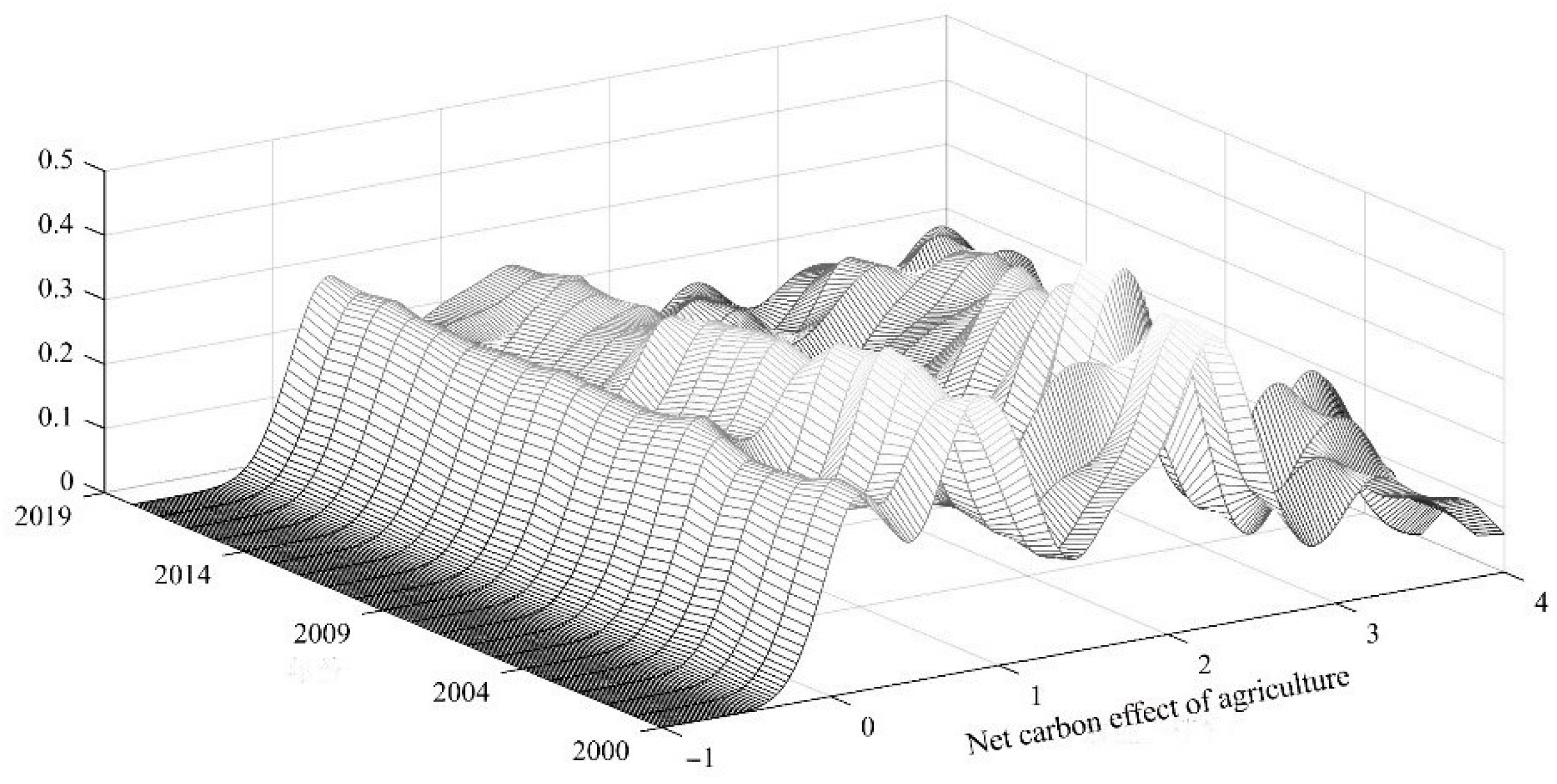
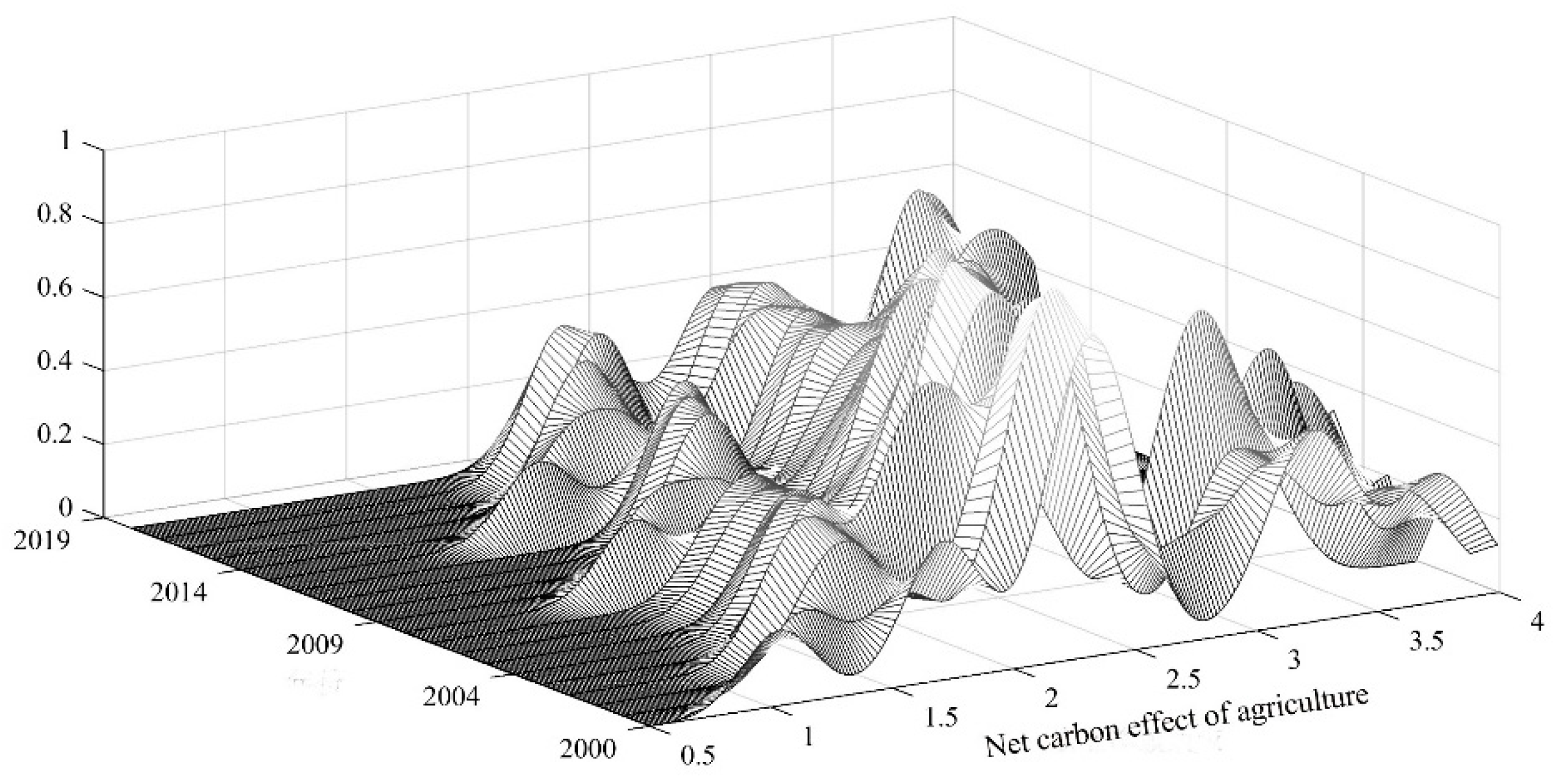
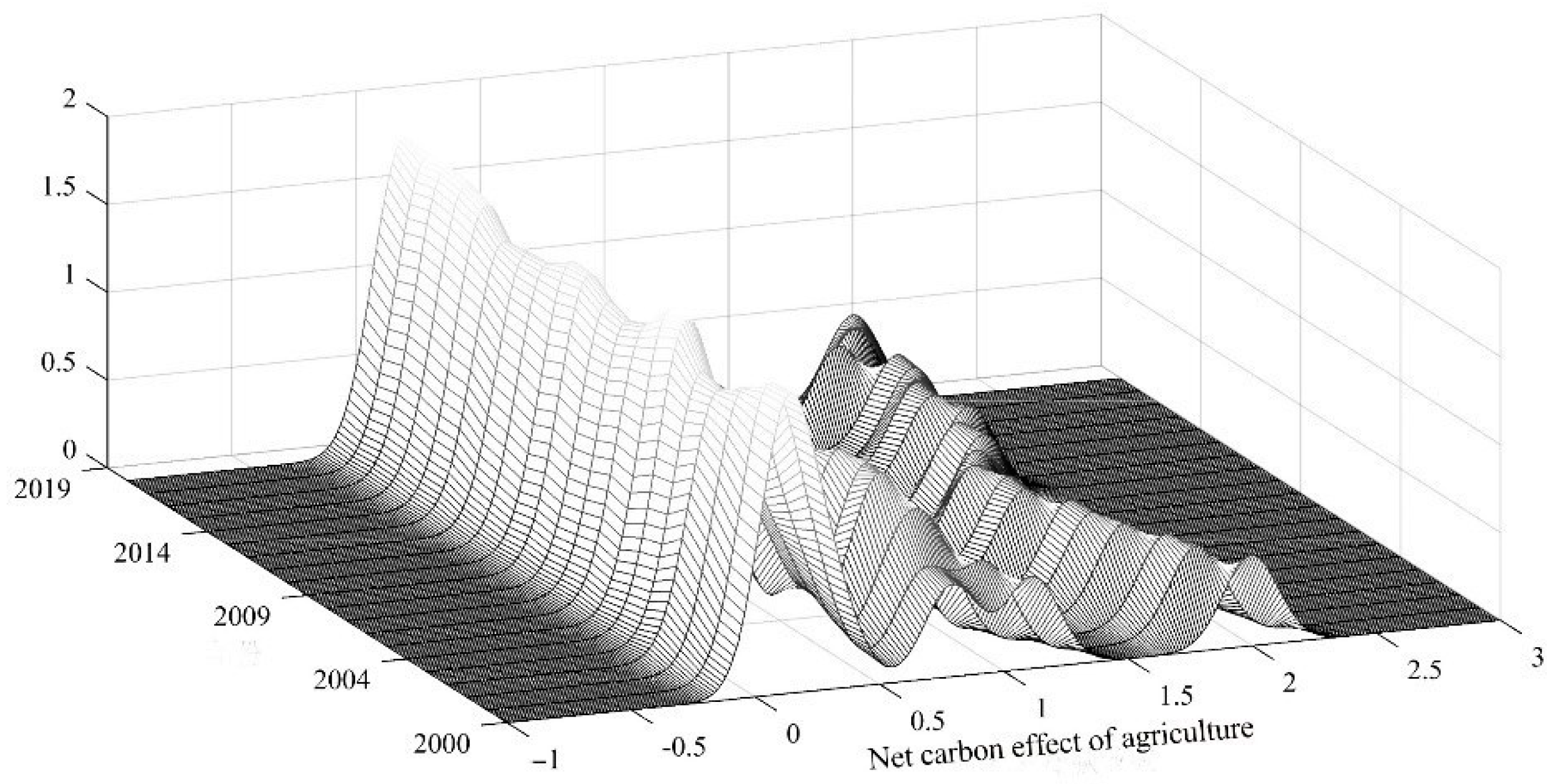
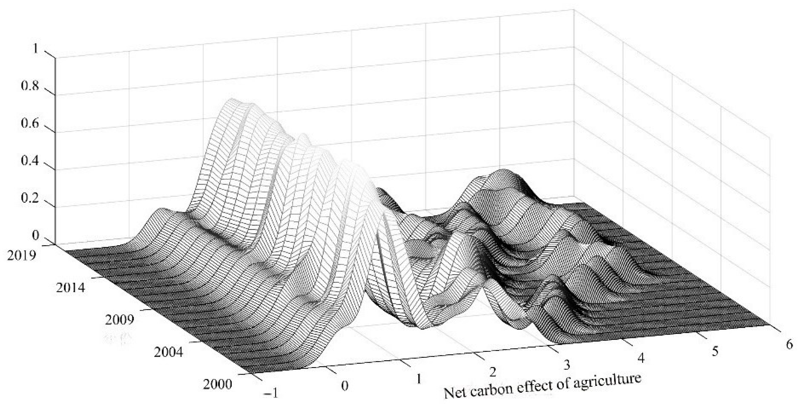
5.1. Time Evolution Based on Kernel Density Estimation

In order to characterize the time-varying process of the absolute differences in the net agricultural carbon effect across areas, the Gauss kernel function was used to estimate its kernel density, which is shown in Figure 3. The kernel density was then estimated using the Gauss kernel function to illustrate the dynamic evolution of the net agricultural carbon effect in China through its distribution location, distribution trend and distribution extensibility. For the country as a whole, the right-skewed distribution of the net agricultural carbon effect in the 31 provinces of China is gradually becoming more pronounced in terms of distribution position. This indicates that the net agricultural carbon sink in high-level areas is increasing, and the number of areas is also increasing. In terms of distribution, the overall kernel density curve shows a decreasing peak and increasing width, indicating that the absolute differences in the net agricultural carbon effect in China are increasing. In particular, the sample period is characterised by multiple peaks, implying a certain gradient of differences in the net carbon effect of agriculture in China. Gao examined agricultural total factor productivity from the perspective of carbon sink and proposed that the three regions showed a decreasing development trend from the east to the west. The agricultural development in the central region has spread more via Eastern science and technology, while the growth was slower in the western region with less spillover [54]. In terms of the extension of the distribution, the overall kernel density shows a right trailing phenomenon over time. This indicates that the gap between China’s net agricultural carbon sink and the average has widened, with the capacity of areas with high net agricultural carbon sinks increasing faster, while the carbon sink capacity of areas with low net agricultural carbon sinks has decreased.

From Figure 4, the distribution of the net agricultural carbon effect in the main food-producing areas shows an overall rightward trend and a progressively more right-skewed distribution. This indicates that the net agricultural carbon sink in the area has increased over the sample period, with the numbers of high-value areas and the provinces increasing. In terms of the distribution, the peak of the kernel density curve of the net agricultural carbon effect in the area is decreasing, while there is a widening trend and the rate of widening is increasing, with the characteristic of one main peak and many side peaks. It means that the absolute difference in the net agricultural carbon effect between provinces within the main grain-producing areas is increasing, and there is a certain gradient of difference. In terms of distribution extension, the overall kernel density shows a right-trailing phenomenon over time, indicating a gradual concentration of net agricultural carbon sinks in higher-value areas and a possible polarization trend in the future [55].

As can be seen from Figure 5, the kernel density curve of the net carbon effect in the main grain-marketing area does not show an obvious rightward shift in terms of distribution location, which indicates that the net carbon effect of agriculture in this area does not change much. However, in terms of the distribution trend, the peak of the kernel density curve shows a decreasing trend, while there is a widening trend with the characteristic of one main peak and one side peak, and the side peaks have lower values. It indicates that the unevenness of the net agricultural carbon effect among the provinces within the main grain-marketing area is increasing, showing a certain trend in dispersion. In terms of the extension of the distribution, there is a right-trailing phenomenon in the later part of the sample examination, which implies that the net agricultural carbon effect within the main grain-marketing areas has polarised over time.

As can be seen from Figure 6 below, the net carbon effect of agriculture in the balanced production and marketing areas shows a rightward shift in terms of distribution that indicates that the net carbon sink of agriculture in this area is increasing. In terms of distribution dynamics, the peak of the nuclear density curve has decreased, and its peak decreased more in the pre-sample period. The one main peak, many side peaks feature is obvious, and the side peaks are all low. However, as time passes, the peak of the kernel density curve of the net carbon effect of agriculture in the balanced production and marketing areas does not drop significantly in the later part of the sample. This implies that the absolute differences in the net agricultural carbon effect between provinces within the main grain-marketing areas were increasing and showing some dispersion in the early part of the sample but that the degree of absolute differences decreased in the late part of the sample. In the field of the extension of the distribution, similar to the development of the main grain-marketing area, the balanced areas show a right-trailing phenomenon at the end of the sample, which means that provinces with higher levels of net agricultural carbon sinks coexist with provinces with lower levels within the balanced production and marketing areas.

5.2. State Evolution Based on Markov Chain Analysis

(1) Traditional Markov chain analysis. The net agricultural carbon sinks of 31 provinces in China were classified into 4 classes: low, medium-low, medium-high and high; the state transfer probability matrix of the net agricultural carbon effect in China during the sample period was calculated separately; and the results are shown in

Table 4. Traditional Markov transfer probability matrix for the net carbon effect of agriculture.

Time Span	Category	Low	Medium-Low	Medium-High	High
T = 1	Low	0.8947	0.1053	0.0000	0.0000
	Medium-low	0.0132	0.8750	0.1118	0.0000
	Medium-high	0.0000	0.0066	0.7697	0.2237
	High	0.0000	0.0000	0.0301	0.9699
T = 2	Low	0.8750	0.1250	0.0000	0.0000
	Medium-low	0.0069	0.8542	0.1389	0.0000
	Medium-high	0.0000	0.0139	0.6806	0.3056
	High	0.0000	0.0000	0.0317	0.9683
T = 3	Low	0.8676	0.1324	0.0000	0.0000
	Medium-low	0.0074	0.8382	0.1544	0.0000
	Medium-high	0.0000	0.0147	0.5441	0.4412
	High	0.0000	0.0000	0.0336	0.9664
T = 4	Low	0.8672	0.1328	0.0000	0.0000
	Medium-low	0.0156	0.7969	0.1875	0.0000
	Medium-high	0.0000	0.0234	0.4688	0.5078
	High	0.0000	0.0000	0.0268	0.9732
T = 5	Low	0.8500	0.1500	0.0000	0.0000
	Medium-low	0.0250	0.7750	0.2000	0.0000
	Medium-high	0.0000	0.0250	0.3917	0.5833
	High	0.0000	0.0000	0.0190	0.9810

. As can be seen from Table 4, the elements on the main diagonal are the probabilities that the type of net agricultural carbon effect in each province remains constant, reflecting the stability of the evolution of the net agricultural carbon effect occurring in that province. The elements outside the diagonal of the matrix indicate the probability that the type of net agricultural carbon effect will change for different classes. As the time span increases, the probability values on the diagonal for all types of provinces, except for the high-level areas, show a gradual decline. For example, the probabilities on the main diagonal decreased from P₁₁ = 89.47%, P₂₂ = 87.50% and P₃₃ = 76.97% in the T = 1 period to P₁₁ = 85.00%, P₂₂ = 77.50% and P₃₃ = 39.17% in T = 5. The probabilities on the nondiagonal line of P₁₂ = 10.53%, P₂₃ = 11.18% and P₃₄ = 22.37% in period T = 1 increased to P₁₂ = 15.00%, P₂₃ = 12.00% and P₃₄ = 58.33% in period T = 5, respectively. This means that the state of the net agricultural carbon effect in each province is highly volatile and has strong internal mobility in its evolution. The probability of the upward shift of the net agricultural carbon effect at each level is greater than the probability of the downward shift, which reflects that the net agricultural carbon effect still has a positive trend: for example, P₁₂ = 10.53% > P₂₁ = 1.32% and P₂₃ = 11.18% > P₃₂ = 0.66% for T = 1 and P₁₂ = 15.00% > P₂₁ = 2.50% and P₂₃ = 20.00% > P₃₂ = 2.50% in T = 5. In addition, the probability of shifting the net carbon effect of agriculture to neighbouring classes in each province is greater than that of leapfrogging, indicating that the improvement of the net carbon effect of agriculture is a gradual process and it is difficult to achieve leapfrogging in the short term. At the same time, there is a possibility that the net carbon effect of agriculture will converge to a high level. The probability of maintaining stability in the high-level provinces remains above 95% in the period of times 1–5, and its probability of P₄₄ = 96.99% in the period of T = 1 is lower than that of P₄₄ = 98.10% in T = 5. It indicates that the net carbon effect of agriculture in the high-level provinces is stable and self-reinforcing, with an increasing tendency to concentrate in the dominant areas [56].

(2) Spatial Markov chain analysis. Given that the traditional Markov chain approach assumes that areas are independent of each other, the issue of spatial correlation is ignored. This section incorporates spatial lag into the traditional Markov chain analysis to determine whether the net agricultural carbon effect in the neighbouring area affects the net agricultural carbon effect transfer in the area.

Table 5. Spatial Markov transfer probability significance test results.

Duration	Value Q	Degree of Freedom	p
1	81.6837	4	0.0000
2	94.7185	4	0.0000
3	112.4287	4	0.0000
4	119.3027	3	0.0000
5	130.2360	2	0.0000

presents the results of the significance tests for the spatial Markov shift probabilities for different time periods. The results show that the Q statistic is significant at 1%, which reveals the existence of a spatial effect in the dynamic evolution of the net agricultural carbon effect in China [57]. In other words, the transfer of the net agricultural carbon effect in one area will be influenced by the net agricultural carbon effect in its surrounding areas. Wu proposed that the agricultural carbon offset rate had a significant positive spillover effect, while the agricultural carbon sequestration capacity of different regions showed the evolution characteristics of mutual promotion and synergistic improvement [58].

Spatial geographical factors influence the dynamic evolution of the distribution of the net agricultural carbon effect in China, and the results are shown in

Table 6. Spatial Markov transfer probability matrix for the net carbon effect of agriculture.

T = 1		Low	Medium-Low	Medium-High	High	T = 5		Low	Medium-Low	Medium-High	High
Low	Low	0.9901	0.0099	0.0000	0.0000	Low	Low	1.0000	0.0000	0.0000	0.0000
	Medium-low	0.0000	0.8333	0.1667	0.0000		Medium-low	0.5000	0.3333	0.1667	0.0000
	Medium-high	0.0000	0.0000	0.4545	0.5455		Medium-high	0.0000	0.2000	0.0000	0.8000
	High	0.0000	0.0000	0.0000	1.0000		High	0.0000	0.0000	0.0000	1.0000
Medium-low	Low	0.7647	0.2353	0.0000	0.0000	Medium-low	Low	0.7037	0.2963	0.0000	0.0000
	Medium-low	0.0000	0.7872	0.2128	0.0000		Medium-low	0.0000	0.6216	0.3784	0.0000
	Medium-high	0.0000	0.0256	0.9487	0.0256		Medium-high	0.0000	0.0323	0.4839	0.4839
	High	0.0000	0.0000	0.0313	0.9688		High	0.0000	0.0000	0.0400	0.9600
Medium-high	Low	0.6667	0.3333	0.0000	0.0000	Medium-high	Low	0.4286	0.5714	0.0000	0.0000
	Medium-low	0.0192	0.9231	0.0577	0.0000		Medium-low	0.0000	0.9250	0.0750	0.0000
	Medium-high	0.0000	0.0000	0.8548	0.1452		Medium-high	0.0000	0.0000	0.6250	0.3750
	High	0.0000	0.0000	0.0000	1.0000		High	0.0000	0.0000	0.0000	1.0000
High	Low	0.0000	1.0000	0.0000	0.0000	High	Low	0.0000	1.0000	0.0000	0.0000
	Medium-low	0.0213	0.9149	0.0638	0.0000		Medium-low	0.0000	0.8378	0.1622	0.0000
	Medium-high	0.0000	0.0000	0.5500	0.4500		Medium-high	0.0000	0.0000	0.0645	0.9355
	High	0.0000	0.0000	0.0682	0.9318		High	0.0000	0.0000	0.0286	0.9714

. From Table 6, it can be seen that the transfer of net agricultural carbon effect does not exist in isolation but is influenced by the net agricultural carbon effect in the surrounding areas. The probability of shifting varies under different net agricultural carbon effects. Without considering the geospatial pattern, P₁₂ = 10.53% in T = 1. This reveals that the net agricultural carbon effect in the area is influenced by changes in neighbouring areas. The spillover effect on the transfer of net agricultural carbon effect to neighbouring areas varies under the influence of geospatial patterns of different net agricultural carbon effects. For example, P_12/2 = 23.53% < P_12/3 = 33.33% < P_12/4 = 1.00% in T = 1 and P_12/2 = 29.63% < P_12/3 = 57.14% < P_12/4 = 1.00% in T = 5, suggesting that the probability of upward shifts in the province increases when the area is in close proximity to a high-level neighbour. This means that areas with a greater net agricultural carbon effect have “demonstration behaviour” and “imitation behaviour” for the surrounding areas [53]. In addition, the net carbon effect of agriculture in high-level areas is also more stable under the influence of different levels of neighbours, which is consistent with the results of traditional Markov analysis. Du also verified that there was a significant spatiotemporal correlation characteristic of carbon neutrality, so local governments should adopt energy-saving and emission reduction measures from nearby local governments with a better performance [59].

6. Conclusions and Recommendations

This paper used the Dagum Gini coefficient, kernel density estimation and Markov chain analysis to reveal the spatial disequilibrium characteristics of the net agricultural carbon effect in China and its dynamic evolution trends on the basis of constructing and measuring the net agricultural carbon sink of Chinese provinces. The conclusions are made as follows. First, the overall net carbon sink of Chinese agriculture is low but shows a fluctuating upward trend. The net agricultural carbon sinks in the main grain-producing areas, the main marketing areas and the balanced production and marketing areas are decreasing in order. The three provinces with the highest net agricultural carbon sinks in the main grain-producing regions are Henan, Heilongjiang and Inner Mongolia. The top three provinces in the main grain-marketing area are Guangdong, Zhejiang and Fujian. The top three provinces in the balanced production and marketing areas are Guangxi, Xinjiang and Yunnan. There are significant differences in net agricultural carbon sinks between different areas. Second, the overall difference in the net carbon effect of agriculture in China is increasing. The inter-regional difference is the most significant source of its difference, with intra-regional differences making the next largest contribution and hypervariable density making a smaller contribution. In terms of inter-regional differences, the largest are between the main production areas and the main marketing areas. In terms of intra-regional differences, the greatest difference in the net agricultural carbon effect is found within the main grain-marketing areas. Third, the right-skewed distribution of the kernel density curve of the net agricultural carbon effect in China gradually becomes more pronounced. The net agricultural carbon sinks in the high-value areas continues to rise, and the peak of the kernel density curve is decreasing and increasing in width and shows a certain degree of rightward trailing, showing that the absolute difference in the net agricultural carbon effect in China is expanding, and there is a certain gradient difference and multi-polar differentiation trend within areas. Fourth, the evolution of the state of the net agricultural carbon effect in China is highly volatile and has strong internal mobility. The probability of upward shift of the net agricultural carbon effect at each level is greater than the probability of downward shift. In addition, the evolution of the state of the net carbon effect of agriculture in China is influenced by spatial and geographical factors. The probability of an upward shift increases when the area is located next to a high level. Under the influence of different levels of neighbours, the net carbon effect of agriculture in high level areas is still more stable.

Based on the conclusions, the following recommendations are put forward. Firstly, according to the actual situation of the level of net carbon sinks in agriculture in different areas, corresponding initiatives to reduce emissions and increase sinks should be planned in accordance with local conditions. Based on their own comparative advantages, each area should formulate targeted emission reduction and sink enhancement plans and explore different low-carbon development paths for agriculture. Secondly, in view of the obvious spatial unevenness and gradient differences in the development of net carbon sinks in agriculture, cooperation and exchange between areas in reducing emissions and increasing sinks in agriculture need to be strengthened. Efforts should be made to narrow the gap in the net carbon effect of agriculture between the main food-producing areas and the main marketing areas. Investment in the development of low-carbon agriculture in the main food marketing areas can be increased to fully explore its endogenous potential. Thirdly, as the evolution of the net agricultural carbon sinks is influenced by spatial and geographical factors, it is necessary to pay attention to the spatial correlation in the development of net agricultural carbon sinks, cultivate the mechanism of competition and interaction between areas, strengthen cross-regional exchanges and cooperation and gradually form a number of replicable and typical models. This way, it will promote the synergistic enhancement of the net carbon effect of agriculture and narrow the differences in its regional development.

We compared the estimation of net carbon effect with that of other studies and found that it was consistent with the research conclusion of Cao et al. (2022) [60]. However, the key factors that affect the temporal and spatial differentiation of agricultural net carbon effect and how to make the net carbon effect of each region gradually converge to a high and stable level and gradually narrow its regional gap are two major issues that need to be discussed and resolved in the future.

References

1. Chen, W.; Wu, F.; Geng, W.; Yu, G. Carbon emissions in China’s industrial sectors. Resour. Conserv. Recycl. 2017, 117, 264–273. [Google Scholar] [CrossRef]
2. Zhu, X.J.; Zhang, H.Q.; Zhao, T.H.; Li, J.D.; Yin, H. Divergent drivers of the spatial and temporal variations of cropland carbon transfer in Liaoning province, China. Sci. Rep. 2017, 7, 13095. [Google Scholar] [CrossRef] [PubMed] [Green Version]
3. Pachiyappan, D.; Ansari, Y.; Alam, M.S.; Thoudam, P.; Alagirisamy, K.; Manigandan, P. Short and long-run causal effects of CO2 emissions, energy use, GDP and population growth: Evidence from India using the ARDL and VECM approaches. Energies 2021, 14, 8333. [Google Scholar] [CrossRef]
4. Alam, N.; Hashmi, N.I.; Jamil, S.A.; Murshed, M.; Mahmood, H.; Alam, S. The marginal effects of economic growth, financial development, and low-carbon energy use on carbon footprints in Oman: Fresh evidence from autoregressive distributed lag model analysis. Environ. Sci. Pollut. Res. 2022, 29, 76432–76445. [Google Scholar] [CrossRef]
5. Dou, X. Low Carbon Agriculture and GHG Emission Reduction in China: An Analysis of Policy Perspective. Theor. Econ. Lett. 2018, 8, 538–556. [Google Scholar] [CrossRef] [Green Version]
6. Du, Z.; Su, T.; Ge, J.; Wang, X. Forest carbon sinks and their spatial spillover effects in the context of carbon neutrality. Econ. Res. 2021, 56, 187–202. [Google Scholar]
7. Antle, J.M.; Stoorvogel, J.J. Agricultural carbon sequestration, poverty, and sustainability. Environ. Dev. Econ. 2008, 13, 327–352. [Google Scholar] [CrossRef] [Green Version]
8. Piao, S.; Huang, M.; Liu, Z.; Wang, X.; Ciais, P.; Canadell, J.G.; Wang, K.; Bastos, A.; Friedlingstein, P.; Houghton, R.A.; et al. Lower land-use emissions responsible for increased net land carbon sink during the slow warming period. Nat. Geosci. 2018, 11, 739–743. [Google Scholar] [CrossRef] [Green Version]
9. Wang, J.; Feng, L.; Palmer, P.I.; Liu, Y.; Fang, S.X.; Bosch, H.; O’Dell, C.W.; Tang, X.P.; Yang, D.X.; Liu, L.X.; et al. Large Chinese land carbon sink estimated from atmospheric carbon dioxide data. Nature 2020, 586, 720–723. [Google Scholar] [CrossRef]
10. Wu, H.; Guo, S.; Guo, P.; Shan, B.; Zhang, Y. Agricultural water and land resources allocation considering carbon sink/source and water scarcity/degradation footprint. Sci. Total Environ. 2022, 819, 152058. [Google Scholar] [CrossRef]
11. Zhu, K.; Zhang, J.; Niu, S.L.; Chu, C.J.; Luo, Y.Q. Limits to growth of forest biomass carbon sink under climate change. Nat. Commun. 2018, 9, 2709. [Google Scholar] [CrossRef] [PubMed]
12. Piao, S.L.; He, Y.; Wang, X.H.; Chen, F.H. Estimation of China’s terrestrial ecosystem carbon sink: Methods, progress and prospects. Sci. China Earth Sci. 2022, 65, 641–651. [Google Scholar] [CrossRef]
13. Singh, B.P.; Setia, R.; Wiesmeier, M.; Kunhikrishnan, A. Chapter 7—Agricultural Management Practices and Soil Organic Carbon Storage. In Soil Carbon Storage; Academic Press: Cambridge, MA, USA, 2018; pp. 207–244. [Google Scholar]
14. Sha, Z.; Bai, Y.; Li, R.; Lan, H.; Zhang, X.; Li, J.; Liu, X.; Chang, S.; Xie, Y. The global carbon sink potential of terrestrial vegetation can be increased substantially by optimal land management. Commun. Earth Environ. 2022, 3, 1038. [Google Scholar] [CrossRef]
15. Lorenz, D.K.; Lal, P.D.R. Carbon Sequestration in Agricultural Ecosystems; Springer International Publishing: Berlin/Heidelberg, Germany, 2018. [Google Scholar]
16. Sun, K.; Cui, Q.; Su, Z. Analysis on the temporal and spatial evolution and influencing factors of the economic value of marine aquaculture carbon sinks in China. Geogr. Res. 2020, 39, 2508–2520. [Google Scholar]
17. Li, G.; Hou, C.; Zhou, X. Carbon Neutrality, International Trade, and Agricultural Carbon Emission Performance in China. Front. Environ. Sci. 2022, 10, 931937. [Google Scholar] [CrossRef]
18. Li, F.; Liu, J.; Liu, W.L.; Liao, S.B. Spatiotemporal Dynamics Analysis of Carbon Emissions From Nighttime Light Data in Beijing-Tianjin-Hebei Counties. J. Xinyang Norm. Univ. (Nat. Sci. Ed.) 2021, 2, 230–236. [Google Scholar]
19. Sui, J.; Lv, W. Crop Production and Agricultural Carbon Emissions: Relationship Diagnosis and Decomposition Analysis. Int. J. Environ. Res. Public Health 2021, 18, 8219. [Google Scholar] [CrossRef] [PubMed]
20. Liang, D.J.; Lu, X.; Zhuang, M.H.; Shi, G.; Hu, C.Y.; Wang, S.X.; Hao, J.M. China’s greenhouse gas emissions for cropping systems from 1978–2016. Sci. Data 2021, 8, 171. [Google Scholar] [CrossRef] [PubMed]
21. Huang, Y.; Su, Y.; Li, R.; He, H.; Liu, H.; Li, F.; Shu, Q. Study of the Spatio-Temporal Differentiation of Factors Influencing Carbon Emission of the Planting Industry in Arid and Vulnerable Areas in Northwest China. Int. J. Environ. Res. Public Health 2019, 17, 187. [Google Scholar] [CrossRef] [Green Version]
22. West, T.O.; Marland, G. A synthesis of carbon sequestration, carbon emissions, and net carbon flux in agriculture: Comparing tillage practices in the United States. Agric. Ecosyst. Environ. 2002, 91, 217–232. [Google Scholar] [CrossRef]
23. Shi, R.B.; Irfan, M.; Liu, G.L.; Yang, X.D.; Su, X.F. Analysis of the Impact of Livestock Structure on Carbon Emissions of Animal Husbandry: A Sustainable Way to Improving Public Health and Green Environment. Front. Public Health 2022, 10, 835210. [Google Scholar] [CrossRef] [PubMed]
24. Boontiam, W.; Shin, Y.; Choi, H.L.; Kumari, P. Assessment of the Contribution of Poultry and Pig Production to Greenhouse Gas Emissions in South Korea Over the Last 10 Years (2005 through 2014). Asian Australas. J. Anim. Sci. 2016, 29, 1805–1811. [Google Scholar] [CrossRef] [Green Version]
25. Dunkley, C.S.; Dunkley, K.D. Greenhouse Gas Emissions from Livestock and Poultry. Agric. Food Anal. Bacteriol. 2013, 3, 17–29. [Google Scholar]
26. Parker, R.W.R.; Blanchard, J.L.; Gardner, C.; Green, B.S.; Hartmann, K.; Tyedmers, P.H.; Watson, R.A. Fuel use and greenhouse gas emissions of world fisheries. Nat. Clim. Change 2018, 8, 333–337. [Google Scholar] [CrossRef]
27. Wang, Q.; Wang, S. Carbon emission and economic output of China’s marine fishery: A decoupling efforts analysis. Mar. Policy 2022, 135, 4831. [Google Scholar] [CrossRef]
28. MacLeod, M.J.; Hasan, M.R.; Robb, D.H.F.; Mamun-Ur-Rashid, M. Quantifying greenhouse gas emissions from global aquaculture. Sci. Rep. 2020, 10, 11679. [Google Scholar] [CrossRef] [PubMed]
29. Martin, A.H.; Ferrer, E.M.; Hunt, C.A.; Bleeker, K.; Villasante, S. Exploring Changes in Fishery Emissions and Organic Carbon Impacts Associated with a Recovering Stock. Front. Mar. Sci. 2022, 9, 788339. [Google Scholar] [CrossRef]
30. Johnson, J.M.F.; Franzluebbers, A.J.; Weyers, S.L.; Reicosky, D.C. Agricultural opportunities to mitigate greenhouse gas emissions. Environ. Pollut. 2007, 150, 107–124. [Google Scholar] [CrossRef]
31. Huang, X.Q.; Xu, X.C.; Wang, Q.Q.; Zhang, L.; Gao, X.; Chen, L.H. Assessment of Agricultural Carbon Emissions and Their Spatiotemporal Changes in China, 1997–2016. Int. J. Environ. Res. Public Health 2019, 16, 3105. [Google Scholar] [CrossRef] [Green Version]
32. Zhang, H.; Guo, S.; Qian, Y.; Liu, Y.; Lu, C. Dynamic analysis of agricultural carbon emissions efficiency in Chinese provinces along the Belt and Road. PLoS ONE 2020, 15, e0228223. [Google Scholar] [CrossRef] [Green Version]
33. Xiong, C.H.; Yang, D.G.; Xia, F.Q.; Huo, J.W. Changes in agricultural carbon emissions and factors that influence agricultural carbon emissions based on different stages in Xinjiang, China. Sci. Rep. 2016, 6, 36912. [Google Scholar] [CrossRef] [Green Version]
34. Xiong, C.H.; Yang, D.G.; Huo, J.W.; Zhao, Y.N. The relationship between agricultural carbon emissions and agricultural economic growth and policy recommendations of a low-carbon agriculture economy. Pol. J. Environ. Stud. 2016, 25, 2187–2195. [Google Scholar] [CrossRef]
35. Ghosh, A.; Misra, S.; Bhattacharyya, R.; Sarkar, A.; Singh, A.K.; Tyagi, V.C.; Kumar, R.V.; Meena, V.S. Agriculture, dairy and fishery farming practices and greenhouse gas emission footprint: A strategic appraisal for mitigation. Environ. Sci. Pollut. Res. 2020, 27, 10160–10184. [Google Scholar] [CrossRef]
36. Cui, Y.; Khan, S.U.; Deng, Y.; Zhao, M.J. Regional difference decomposition and its spatiotemporal dynamic evolution of Chinese agricultural carbon emission: Considering carbon sink effect. Environ. Sci. Pollut. Res. 2021, 28, 38909–38928. [Google Scholar] [CrossRef] [PubMed]
37. Shan, T.Y.; Xia, Y.X.; Hu, C.; Zhang, S.X.; Zhang, J.H.; Xiao, Y.D.; Dan, F.F. Analysis of regional agricultural carbon emission efficiency and influencing factors: Case study of Hubei Province in China. PLoS ONE 2022, 17, e0266172. [Google Scholar] [CrossRef]
38. Popp, M.; Nalley, L.; Fortin, C.; Smith, A.; Brye, K. Estimating Net Carbon Emissions and Agricultural Response to Potential Carbon Offset Policies. Agron. J. 2011, 103, 1132. [Google Scholar] [CrossRef]
39. Tian, Y.; Zhang, J.; Luo, X. Regional Comparative Study on Coordination between Net Carbon Benefit and Economic Benefit of Plantation Industry in China. Econ. Geogr. 2014, 34, 142–148. [Google Scholar]
40. Chen, L.; Xue, L.; Xue, Y. Analysis of the spatiotemporal evolution characteristics of China’s agricultural net carbon sink. J. Nat. Resour. 2016, 31, 596–607. [Google Scholar]
41. Xiong, C.; Yang, D.; Huo, J.; Wang, G. Agricultural Net Carbon Effectand Agricultural Carbon Sink CompensationMechanism in Hotan Prefecture, China. Pol. J. Environ. Stud. 2017, 26, 365–373. [Google Scholar] [CrossRef]
42. Pei, J.; Niu, Z.; Wang, L.; Song, X.P.; Huang, N.; Geng, J.; Wu, Y.B.; Jiang, H.H. Spatial-temporal dynamics of carbon emissions and carbon sinks in economically developed areas of China: A case study of Guangdong Province. Sci. Rep. 2018, 8, 13383. [Google Scholar] [CrossRef] [Green Version]
43. Li, B.; Wang, C.; Zhang, J. Dynamic evolution and spatial spillover effect of China’s agricultural net carbon sink efficiency. China Popul. Resour. Environ. 2019, 29, 68–76. [Google Scholar]
44. Weng, L.; Li, W.; Zhang, M.; Tan, J. Spatial and temporal evolution characteristics of net carbon sinks in farmland ecosystems in Jiangsu Province. Resour. Environ. Yangtze River Basin 2022, 31, 1584–1594. [Google Scholar]
45. Dagum, C. Decomposition and Interpretation of Gini and the Generalized Entropy Inequality Measures. Empir. Econ. 1997, 22, 515–531. [Google Scholar] [CrossRef]
46. Huang, J.; Zhong, P.S. Spatial Difference and Dynamic Evolution of the Development Level of New Urbanization in Henan Province. J. Xinyang Norm. Univ. (Philos. Soc. Sci. Ed.) 2022, 6, 1–13. [Google Scholar]
47. Shepero, M.; Munkhammar, J. Spatial Markov chain model for electric vehicle charging in cities using geographical information system (GIS) data. Appl. Energy 2018, 231, 1089–1099. [Google Scholar] [CrossRef]
48. Tian, Y.; Zhang, J. Research on the Equity of Agricultural Carbon Emissions in China’s Provincial Regions. China Popul. Resour. Environ. 2013, 23, 36–44. [Google Scholar]
49. Zhou, J.; Wang, Y.X.; Liu, X.R.; Shi, X.C.; Cai, C.M. Research on spatial and temporal differences of carbon emissions and carbon offsets in China’s provinces based on land use change. Geogr. Sci. 2019, 39, 1955–1961. [Google Scholar]
50. Jiang, F.; Chen, J.M.; Zhou, L.X.; Ju, W.M.; Zhang, H.F.; Machida, T.; Ciais, P.; Peters, W.; Wang, H.M.; Chen, B.Z.; et al. A comprehensive estimate of recent carbon sinks in China using both top-down and bottom-up approaches. Sci. Rep. 2016, 6, 22130. [Google Scholar] [CrossRef] [Green Version]
51. Tian, Y.; Zhang, J. Research on the driving mechanism of agricultural carbon effect from the perspective of geographical division. J. Huazhong Agric. Univ. 2020, 02, 78–87. [Google Scholar]
52. Ding, X.H.; Cai, Z.Y.; Fu, Z. Does the new-type urbanization construction improve the efficiency of agricultural green water utilization in the Yangtze River Economic Belt? Environ Sci Pollut R. 2021, 28, 64103–64112. [Google Scholar] [CrossRef]
53. Han, H.B.; Zhong, Z.Q.; Guo, Y.; Xi, F.; Liu, S.L. Coupling and decoupling effects of agricultural carbon emissions in China and their driving factors. Environ. Sci. Pollut. Res. 2018, 25, 25280–25293. [Google Scholar] [CrossRef]
54. Gao, M.F.; Zheng, J. Measurement of total factor productivity of agriculture in China and analysis of its temporal and spatial differences: Retesting from the perspective of carbon sink. Ecol. Econ. 2021, 37, 98–104. [Google Scholar]
55. Wu, H.; He, Y.; Huang, H.; Chen, W.K. Calculation and Spatial Convergence of Carbon Offset Rate in China’s Planting Industry. China Popul. Resour. Environ. 2021, 31, 113–123. [Google Scholar]
56. Wu, H.; He, Y.; Chen, W.K.; Huang, H. Research on the Spatial Effect and Influencing Factors of China’s Agricultural Carbon Offset Rate: Based on Spatial Durbin Model. Agric. Technol. Econ. 2020, 6, 110–123. [Google Scholar]
57. Cui, Y.; Khan, S.U.; Deng, Y.; Zhao, M.J.; Hou, M.Y. Environmental improvement value of agricultural carbon reduction and its spatiotemporal dynamic evolution: Evidence from China. Sci. Total Environ. 2020, 754, 142170. [Google Scholar] [CrossRef]
58. Wu, H.Y.; He, Y.Q.; Chen, W.K.; Huang, H.J. Spatial effect and influencing factors of China’s agricultural carbon compensation rate. J. Agrotech. Econ. 2020, 3, 110–123. [Google Scholar]
59. Du, P.C.; Hong, Y. Approaches and policy choices for carbon neutrality. China Popul. Resour. Environ. 2022, 32, 35–46. [Google Scholar]
60. Cao, Z.; Huang, F.; Wu, S. Temporal and spatial characteristics of carbon sink effect and production performance of agricultural production in China. Econ. Geogr. 2022, 42, 166–175. [Google Scholar]
Figure 1. Trends in overall, intra-regional and inter-regional difference in the net carbon effect of agriculture.
Sustainability 14 13975 g001
Figure 2. Trends in the overall sources of difference in the net carbon effect of agriculture.
Sustainability 14 13975 g002
Figure 3. National overall net agricultural carbon effect kernel density distribution.
Sustainability 14 13975 g003
Figure 4. Kernel density distribution of the net carbon effect of agriculture in major food-producing areas.
Sustainability 14 13975 g004
Figure 5. Kernel density distribution of the net carbon effect of agriculture in the main food marketing areas.
Sustainability 14 13975 g005
Figure 6. Kernel density distribution of the net carbon effect of agriculture in balanced production and marketing areas.
Sustainability 14 13975 g006