Exploitation of Machine Learning Algorithms for Detecting Financial Crimes Based on Customers’ Behavior

Abstract

Longer-term projections indicate that today’s developing and rising nations will account for roughly 60% of the global GDP by 2030. There is tremendous financial growth and advancement in developing countries, resulting in a high demand for personal loans from citizens. Depending on their needs, many people seek personal loans from banks. However, it is difficult for banks to predict which consumers will pay their bills and which will not since the number of bank frauds in many countries, notably India, is growing. According to the Reserve Bank of India, the Indian banking industry uncovered INR 71,500 in the scam in the fiscal year 2018–2019. The average lag time between the date of the occurrence and its recognition by banks, according to the statistics, was 22 months. This is despite harsher warnings from both the RBI and the government, particularly in the aftermath of the Nirav Modi debacle. To overcome this issue, we demonstrated how to create a predictive loan model that identifies problematic candidates who are considerably more likely to pay the money back. In step-by-step methods, we illustrated how to handle raw data, remove unneeded portions, choose appropriate features, gather exploratory statistics, and finally how to construct a model. In this work, we created supervised learning models such as decision tree (DT), random forest (RF), and k-nearest neighbor (KNN). According to the classification report, the models with the highest accuracy score, f-score, precision, and recall are considered the best among all models. However, in this work, our primary aim was to reduce the false-positive parameter in the classification models’ confusion matrix to reduce the banks’ non-performing assets (NPA), which is helpful to the banking sector. The data were graphed to help bankers better understand the customer’s behavior. Thus, using the same method, client loyalty may also be anticipated.

1. Introduction

Machine learning (ML) is one of the most exciting recent technologies. It is a rapidly growing area of data science that deals with machines that learn from their experiences. One such challenge is to assist with making predictions for financial data [1]. In other words, ML is related to computer applications that automatically enhance their overall performance through experiences [2]. It has the potential to develop systems that can automatically adapt and customize themselves to individual users.

Due to the enormous amount of data that organizations have access to and to the expansion of hardware capability, machine learning approaches have improved in strength and efficiency in regard to handling more challenges in our society. The detection of credit card (CC) applications (fraudulent applications) and transaction fraud uses a variety of machine learning and data mining techniques. These include the Bayesian network, decision tree (DT), support vector machine (SVM), k-nearest neighbor (KNN), neural network, hidden Markov model (HMM), artificial immune systems (AIS), and a self-organizing map (SOM).

A fraud control mechanism’s main objective is to keep sophisticated technology safe against fraud by avoiding it in the first place. Nevertheless, this approach is insufficient to avoid fraud. It is frequently advised to use fraud detection to increase the security of technical systems. As fraudulent transactions take place in the system, CC fraud detection finds them, detects them, and notifies the system administrator. This sensitive and fascinating procedure necessitates accurate identification and detection capabilities. It can be difficult for a machine or system to recognize CC fraud. A system must be thoroughly trained with appropriate data in order to successfully complete the fraudulent detection procedure. Machine learning is the process of a system or machine learning through statistical approaches such as clustering, regression, and classification. The following factors led to our decision to use machine learning-based algorithms for detecting fraud:

• It detects frauds without fail;
• It can conduct real-time streaming;
• It requires less time for authentication procedures;
• It can identify hidden connections in data.

The loan is a vital product of the banking system. All banks are searching for powerful commercial strategies to influence customers to use their loans. There are some customers that behave negatively after their application form is approved. To handle these type of customers, banks have to develop techniques to predict their behaviors. For this purpose, ML algorithms have an excellent performance and are widely utilized by the banking.

Supervised learning methods concentrate on exploring different past transactions, which are reported by the cardholder or CC company, to predict whether any new transaction is fraudulent or not. This method needs a dataset that has been divided between fraud and non-fraud observations. Unsupervised learning methods require an organization of unlabeled data into similarity groups called clusters. They operate under the premise that anomalies represent fraudulent transactions. Clustering makes it possible to identify various data distributions for which various predictive models should be applied.

Semi-supervised ones combine the prior strategies to benefit from recalling previous fraudulent transactions and utilizing unsupervised techniques to identify future fraudulent transaction patterns. To identify fraudulent CC transactions, a hybrid technique that integrates many ML techniques, such as SVM, MLP, random forest regression, autoencoder, and isolation forest, can be used.

Our work has made the following significant contributions.

• The fraud detection team’s heavy workload of data processing is eliminated by machine learning. The findings aided the team’s research, insights, and reporting.
• The following ML methods were built and evaluated:
• SVM, KNN, DT, NB, and LR.

Using fresh data retrieved from the form, banks may discover the default behavior of consumers and anticipate whether a person would commit fraud or not. Appendix A contains lists all the abbreviations used in our manuscript.

The rest of the paper is organized as follows: Section 2 discusses the related work. In Section 3, we discuss the methodology, and Section 4 contains results and discussion. Section 5 contains the conclusion of the proposed work. The last section contains the future direction of the proposed work.

2. Related Work

In our paper, we resolved this problem by the method of loan default prediction with ML algorithms [3]. In the banking and financial sectors, loan prediction is a popular issue. Credit rating has become a critical component in today’s competitive economic system. Recent advances in data science and artificial intelligence have heightened academic interest. It currently focuses on credit risk assessment and loan forecast. The increasing loan demand needs better credit scoring and loan prediction algorithms [4]. Decades of research have gone into determining individual credit ratings. Experts were employed in the past and models rely on expert judgements, but, currently, the emphasis is on automation. For credit rating and risk assessment, ML algorithms and neural networks are being used [5,6]. This topic has seen several notable successes, setting the path for future studies.

The paper [7,8] looked at a range of approaches, including SVMs, KNNs, artificial neural networks (ANN), logistic regression (LR), ANN with stochastic gradient (SGD), boosting, RF, naive Bayes (NB), and others, and concluded that there is not one best method for all. The authors examined credit ratings for home loans and came to the following conclusions [9]: credit applications that do not meet standards are usually denied owing to default risk.

Low-income applicants have a higher chance of being accepted and repaying their loans on time. The author of [10] employed an ML-DT classification approach to build their model, and some authors have followed a distributed tree method [11,12]. This was followed by exploratory data analysis, missing value imputation, and finally developing a model and evaluating it [4,9]. Using a public test, the authors achieved an accuracy of 81%. With a data partition of 90:10, the maximum precision was 78.08% precision and 96.4% recall. The 80:20 split was picked as the best because of its high accuracy and recall value [13].

The authors of [14] used exploratory data analysis in their work. The major goal of the paper was to categorize and evaluate loan applicants. Using seven graphs, the authors found that the majority of loan applicants favored short-term loans. Based on the article’s benchmarking models, the authors of [15] claimed that SVMs can outperform LR and RF [16]. Using the models LR, RF, GB, etc., they also illustrated the need of data quality checks, such as data analysis and cleaning, prior to modelling. According to the paper, the algorithm and feature selection are two significant variables to consider when granting a loan. The authors used data mining techniques to create a model for predicting loan risk in their paper [17]; they used three algorithms, namely J48, NB, and Bayes net. J48 was rated the best algorithm for the challenge because of its high accuracy (78.37%) and low mean absolute error (0.34). Aditi Kacheria et al. used NB modelling for their model. They used KNN and binning to increase data quality and classification accuracy. The missing data were handled using KNN, and the abnormalities were eliminated by binning. According to their research, most local banks in the Czech and Slovak Republics adopt logit-based models [18,19]. Other approaches, such as CART or neural networks, are commonly used to help choose variables and evaluate model quality. Less or no application of the KNN approach is concluded by the authors. In his work [18], Yu Li compared the XGBoost technique to logistic regression. It offers better model discrimination and model stability than an LR model, as the article claims. In today’s scenario, when data are large, we can apply big data techniques to identify key persons [20] for fraud detection. Before that, we can apply an ensemble of clustering approaches for the faster detection of outliers [21,22,23,24,25].

Datasets for credit cards include transactional details such account numbers, card types, types of purchases, locations and times of transactions, client names, merchant codes, transaction sizes, etc. Several researchers utilized these data as a variable to decide if the transaction was legal or fraudulent or to spot outliers that required further examination. To identify behavioral fraud, Bolton and Hand [26] developed two clustering techniques: peer group analysis and break-point analysis. Peer group analysis was used by Weston et al. [27] to identify outliers and questionable transactions in real CC transaction data. Scatter search and genetic algorithms were used by Duman and Ozcelik [28] to reduce the number of transactions that were incorrectly categorized. Genetic programming was also used by Ramakalyani and Umadevi [29] to identify fraudulent card transactions. In order to create fuzzy logic rules, Bentley et al. [30,31,32,33,34,35] introduced a fuzzy Darwinian detection model based on genetic programming.

Using an HMM first trained with the cardholder’s typical behavior, Srivastava et al. [36] analyzed a series of CC transactions and demonstrated how the model may be applied to the identification of fraud. With the same goal in mind, Esakkiraj and Chidambaram [37] and Mishra et al. [38] used HMM in other investigations. Brabazon et al. [39] and Wong et al. [40] examined artificial immune systems for the identification of fraudulent transactions, mimicking the immune system’s capacity to distinguish between the self and non-self. Association rules were utilized by Sánchez et al. [41] to gather information regarding fraudulent and illegal card transactions.

A cost-sensitive DT strategy for fraud detection was put forth by Sahin et al. [42]. For the purpose of detecting CC fraud, Bahnsen et al. [43] suggested a cost-sensitive method based on Bayes minimum risk. The best method for spotting fraud tendencies, according to Pasarica [44], is to classify data using a support vector machine and a Gaussian kernel. Sahin and Duman [45] compared decision trees and support vector machine approaches using the three algorithms CART, C5.0, and CHAID. They found that decision trees, particularly the CART algorithm, performed better than support vector machine techniques. For the purpose of identifying fraud, Ganji and Mannem [46] devised a data stream outlier identification technique based on reverse KNN.

Hormozi et al. [47] presentation of a CC fraud detection system utilized the Hadoop and MapReduce architecture in conjunction with the negative selection method, one of the artificial immune system techniques. A real-time CC fraud detection model was created by Quah and Sriganesh [48] utilizing self-organizing maps to separate fraudulent activity from typical behavioral patterns. Kundu et al. [49] used a hybridization of the BLAST and SSAHA algorithms as a profile analyst and a deviation analyzer for CC fraud. An adaptive system for detecting CC fraud was created by Sherly and Nedunchezhian [50] utilizing the Bootstrapped Optimistic Algorithm for Tree building (BOAT). VFDT, a sort of online decision tree invented by Minegishi and Niimi [51], was used to identify fraudulent credit card use. Active learning techniques used to categorize credit card fraud transactions were introduced by Carcillo et al. [52]. The performance and detection accuracies of these techniques were examined by the authors.

Numerous studies [53,54] concentrated on neural network applications for CC fraud detection. Ogwueleka [55] employed an ANN with a rule-based component, whereas Patidar and Sharma [56] used an ANN tuned using genetic algorithms. Various studies mixed a neural network with other techniques. Fuzzy neural networks were established on parallel machines by Syeda et al. [57] with the aim of accelerating rule generation for customer-specific CC fraud detection. On the basis of real-world financial data, Maes et al. [58] comparison of artificial neural networks and Bayesian belief networks revealed that the latter can identify 8% more fraudulent transactions. Transaction aggregation was introduced by Whitrow et al. [59], and its usefulness was demonstrated. Additionally, they demonstrated that random forests outperform alternative techniques, including KNN, LR, and SVM.

In a comparison study involving LR, SVM, and RF, Bhattacharyya et al. [60] found that RF performed better than the other two techniques. The CART algorithm outperformed the competition, according to Subashini and Chitra [61], who compared DT (CART and C5.0), SVM with polynomial kernels, LR, and Bayesian belief networks. Using a simple linear discriminant analysis for CC identification for the first time, Mahmoudi and Duman [62] recently proposed a modified Fisher discriminant function and updated it to be more sensitive to false negatives.

A framework for detecting CC fraud using ML algorithms was presented by Tanouz et al. [63]. The performance of the suggested strategies was evaluated in this study by the authors using the dataset of European cardholders. In addition, the authors adopted an under-sampling strategy to address the problem of class imbalance that existed in the dataset used. The RF and LR are two ML techniques taken into consideration in this paper. The primary performance metric employed by the researchers was accuracy. The findings showed that the RF method had a 91.24% accuracy rate for fraud detection. The accuracy of the LR technique, in contrast, was 95.16%. The confusion matrix was also calculated by the authors to determine if these suggested strategies worked best for the positive and negative classes. The findings indicated that further research is needed to address the issue of class imbalance that exists in the dataset of European CC holders.

Numerous studies have put forth various solutions to the problem of the imbalanced class in CC fraud detection. In order to remove extreme outliers from minority class data, Padmaja et al. [64] suggested a fraud detection method employing k-reverse nearest neighbor (KRNN) [65,66,67,68,69,70,71,72]. Second, hybrid resampling—under sampling the majority class and oversampling the minority class—was applied to the dataset. Several classifiers, including the NB, C4.5 DT, and KNN classifiers, were trained using the resampled data [73,74,75,76,77,78,79,80,81].

Using pattern recognition algorithms, the authors of article [82] were able to distinguish between several brands of distilled spirits (PCA and ANN). In this study, we compared the recognition success rates of many popular algorithms. The back propagation neural network (BPNN) has the highest accuracy in recognition. However, the BPNN’s poor convergence speed makes it vulnerable to entering a local minimum. To counteract the BPNN’s drawback, a more disordered variant was tested. When compared to the BPNN, the chaotic BPNN has a convergence speed that is 75.5 times faster.

The dynamic state estimate of generators under cyber-attacks is the focus of the paper [83]. After modelling attacks and incorporating them into the DSE of generators, we used the RCKF algorithm to estimate the dynamic states of the generators while they are under attack from cyber actors of varying sophistication. This is the first study looking into the DSE of generators when under cyber-attack, according to the authors. The following inferences can be made from the test results on the two IEEE test systems. The RCKF has two main advantages over the CKF: (1) It can execute DSE on generators even when cyber assaults are present; (2) it has superior filtering capabilities. (3) If a DSE method such as CKF is not prepared to deal with cyber threats, its estimation performance may suffer greatly. Table 1 contains a comparison of related works on fraud detection.

Table 1. Comparison of related works on fraud detection.

S. No.	Ref.	Methodology	Dataset Used	Result
1	[22]	GAN	Set of numbers included 492 suspect instances and 284,315 legitimate ones.	99.1 (Area Under ROC (AUROC)) 99.3 (Average Precision (AP))
2	[31]	CNN	CDR data collected from a real mobile network operator.	82% (Accuracy)
3	[32]	CNN	A commercial bank’s actual dataset, featuring 5 million B2C transactions.	91% (Precision) 94% (Recall)
4	[33]	Autoencoder	Statlog (German credit data) data set.	84.1 (Accuracy)
5	[34]	Autoencoder	Dataset A from SAP ERP has 307,457 journal entries, while Dataset B includes 172,990 journal entries.	32.93 ((Dataset A) f1-score) 16.95 ((Dataset B) f1-score)
6	[35]	Autoencoder	Collection of data pertaining to the use of credit cards. A supplementary data collection of users’ responses to advertisements.	When compared to single and variational autoencoders, stacked autoencoders performed better.
7	[65]	Autoencoder	Statistical information from Europe. As a testing dataset, we employed 490 fraud and 490 legitimate transactions, whereas the training dataset had 700 authentic transactions.	89% (accuracy)
8	[66]	Combination of an autoencoder and a restricted Boltzmann machine.	A database with 1000 transactions in German. There are 690 deals in the Australian data collection. There is a total of 284,807 deals in the European dataset.	0.9603 (AUC’s score based on AE) 0.9505 (AUC’s score based on RBM for European Dataset)
9	[67]	RNN	Data collected from UnionPay transactions during a three-month period.	Effectiveness is high despite the unbalanced nature of the data.
10	[68]	Random forest and LSTM-RNN.	Exact credit card transactions made between March and May of 2015 were collected in this dataset.	For offline transactions, LSTM excels.
11	[69]	GAN	Set of numbers included 492 suspect instances and 284,315 legitimate ones.	With a slight increase in false positives, sensitivity has increased.
12	[73]	Deep neural network	284,807 transactions conducted by European cardholders in 2013 were included in this data collection.	96.34% (accuracy) 94.06% (recall)
13	[74]	Deep neural network	Dataset containing more than 900 million between January 2014 and June 2015.	The value detection rate (VDR), the true false positive ratio (TFPR), and AROC (area of receiver operating characteristic) for March, April, and May 2015) were provided.
14	[75]	Neural network training in BP was improved using the whale method.	Dataset containing 284,315 genuine transactions and 492 fraud cases.	98.04% (F-Measure)
15	[76]	LSTM-RNN, CNN	A dataset produced by a Brokerage firm. 1000 samples for training with 250 attributes.	0.8 (F1 score for CNN) 0.91 (F1 score for LSTM-RNN)
16	[77]	LSTM-RNN, CNN	Statlog (German credit data) data set.	0.8 (F1 score for CNN) 0.92 (F1 score for LSTM-RNN)

3. Methodology

This research was based on the examination of bank loan data obtained through Lending Club, an online banking platform that enables borrowers to obtain loans from willing investors at a lower interest rate. The source of the dataset is real and public, and one can find it at https://www.kaggle.com/datasets/wordsforthewise/lending-club (accessed on 17 June 2021). This platform is a type of marketplace where it helps to match the borrowers with the investors by originating peer-to-peer connection. The aim of this research was to identify the bad loan applicants who are applying for the loans. We used the Python language and its libraries on the Jupyter Notebook, which is an open-source platform, and it is so convenient to use and has a higher performance as well. In this paper, we compare the accuracy of different algorithms and developed a system that can perform the early prediction of customers’ behaviors with a higher accuracy and f-score as well. The main motive of our research was to minimize the false-positive parameter, i.e., Type-1 error and, depending on the accuracy, f-score, and false-positive parameters. We chose the algorithm that performed the best for predicting whether the customer was able to pay the loan or not. In this way, banks can find the default behaviors in the sooner degree and conduct the corresponding actions to minimize the feasible loss.

Our proposed system is mentioned in Figure 1 in the form of a model diagram. Figure 1 indicates the flow of the research carried out in building the model. The inputs to our algorithms are the numeric features that we developed based on the financial record data. To predict the customer’s behavior, we used all major supervised learning algorithms, i.e., DT, NB, RF, KNN, LR, and SVM. We built a model and then compared the accuracy, f-score, and false positive parameters of these algorithms. After training the model, we evaluated these models using the test data on the basis of the classification report, confusion matrix, and accuracy score. After that, we predicted whether a person would conduct fraud or not using the classification report and accuracy score. The machine learning algorithms used in this paper are described below.

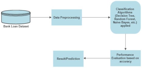
Figure 1. Model diagram.

3.1. Logistic Regression

Classification issues are solved using the supervised learning approach known as logistic regression. In classification issues, dependent variables are discrete or binary numbers, such as 0 or 1. The algorithm for logistic regression uses categorical variables such as 0 or 1, Yes or No, True or False, spam or not spam, etc. It uses probability as the basis for its predictive analytic technique. Although it is a form of regression, logistic regression differs from the linear regression algorithm in terms of how it is applied. A sophisticated cost function called the logistic or sigmoid function is used in logistic regression. To model the data in logistic regression, this sigmoid function is employed. This is a representation of the function:

$$\mathrm{f}\left(\mathrm{x}\right)=\frac{1}{1+{\mathrm{e}}^{-\mathrm{x}}}$$

where f(x) = output between the 0 and 1 value, x = input to the function, and e = base of natural logarithm.

To compute the computational complexities of different ML models, we took the following assumptions: n = number of training examples, m = number of features, n′ = number of support vectors, k = number of neighbors, and k′ = number of trees.

Computational complexities of logistic regression are:

• Train time complexity = O(n × m)
• Test time complexity = O(m)
• Space complexity = O(m)

3.2. Support Vector Machine

SVM is a tool for both classification and regression issues. However, it is largely employed in machine learning classification issues. The SVM algorithm’s objective is to establish the best line or decision boundary that can divide n-dimensional space into classes, allowing us to quickly classify fresh data points in the future. A hyperplane is the name given to this optimal decision boundary. SVM selects the extreme vectors and points that aid in the creation of the hyperplane. Support vectors, which are used to represent these extreme instances, form the basis for the SVM method. Computational complexities of support vector machines are:

• Train time complexity = O(n²)
• Test time complexity = O(n′ × m)
• Space complexity = O(n × m)

3.3. Decision Tree

Decision trees are a sort of supervised machine learning in which the training data are continually segmented based on a particular parameter, with you describing the input and the associated output. Decision nodes and leaves are the two components that can be used to explain the tree. The choices or results are represented by the leaves. The data are divided at the decision nodes. Computational complexities of decision trees are:

• Train time complexity = O(n × log(n) × m)
• Test time complexity = O(m)
• Space complexity = O(depth of tree)

3.4. Random Forest

With the use of the training dataset, it produces decision trees with various levels. The data for the decision tree are used to construct the training data and testing data, in which a method known as “ensemble” is used to combine various models to produce the output. Computational complexities of random forest are:

• Train time complexity = O(k’ × n × log(n) × m)
• Test time complexity = O(m × k’)
• Space complexity = O(k’ × depth of tree)

3.5. K-Nearest Neighbor

K-nearest neighbor is a machine learning approach for classification and regression that is based on statistics. K-nearest training samples are the input for KNN classification, while class membership is the result. K is a positive integer that is typically small in KNN.

The following are the stages involved with KNN:

• Data loading.
• Initialization of the K value.
• To obtain the predicted class, iteration from 1 to the total number of data points of training data.

(i) Calculating the distance between training data (each row) and test data. Different metrics for measuring distance are available, including Euclidean, Manhattan, Chebyshev, and cosine.

(ii) Distance values will determine how the calculated distances are arranged in order (ascending).

(iii) From the sorted array, one can obtain the top k rows.

(iv) From these rows, the most common class may be found.

(v) The predicted class is attained.

Computational complexities of KNN are:

• Train time complexity = O(k × n × m)
• Test time complexity = O(n × m)
• Space complexity = O(n × m)

3.6. Naive Bayes

The concept of conditional probability is the foundation of the naive Bayes algorithm. The idea behind conditional probability is to calculate the likelihood of an event occurring given the occurrence of another event. The algorithm’s job is to evaluate the evidence, decide which class each thing is most likely to belong to, and then assign each one of those labels. Predictive probability models use the idea of a conditional probability distribution P (Y|X), from which Y can be predicted from X. The Bayes rule is defined as

$$P(A|B)=\frac{P(B|A)P\left(A\right)}{P\left(B\right)}$$

Computational complexities of naive Bayes are:

• Training time complexity = O(n × m)
• Test time complexity = O(m)

The classification report assesses the predictions of an algorithm, i.e., how accurate the forecasts were. True positives (TP), false positives (FP), true negatives (TN), and false negatives (FN) forecast the metrics of a categorization report.

Precision = TP/(TP + FP).

(1)

Precision is intuitively the ability of the grader not to label a negative sample as positive.

Recall = TP/(TP + FN).

(2)

Recall is intuitively the ability of the grader to locate all positive samples.

• The F-beta score can be conceptualized as a weighted harmonic mean of recall and precision, where TP is the number of true positives, and the best and worst values are 1 and 0, respectively.
• CM is a performance metric for ML classification tasks with two or more output classes. In Table 2, there are four distinct projections and actual values.
  Table 2. Confusion matrix (CM).

  	Predicted Positive	Predicted Negative
  Actual positive	TP	FN
  Actual negative	FP	TN

• The accuracy score is calculated by dividing the total number of input samples by the number of accurate predictions. The model with the highest accuracy score outperforms the others. It only works when there are an equal number of samples in each class.

We have also used the CAP curve to visualize all the six classification models for more analysis and better understanding.

CAP stands for cumulative accuracy profile. The CAP curve is used to visualize a model’s discriminative power. The larger the area covered between the random model (aR) and perfect model (aP) line is, the better the model compared to the other models.

4. Results and Discussion

The dataset of the Lending Club that we took from the website was firstly analyzed using the Pandas Dataframe. This gave the detailed information of the datasets, such as their size, types, feature information, etc. The details of the dataset that we used here are shown in Table 3. For the visualization of the data, we conducted an exploratory data analysis to obtain information about the correlation between the features of the datasets.

Table 3. Data of the loan borrowers.

Credit Policy	Log Annual.Inc.	Days.with. Cr.Line	Purpose	Int.Rate	Installment	Dti	Fico	Revol.Bal	Revol.Util
1	debtconsolidation	0.12	829.1	11.35	19.48	737	5639.96	28,854	52.1
1	creditcard	0.11	228.22	11.08	14.29	707	2760	33,623	76.7
1	debtconsolidation	0.14	366.86	10.37	11.63	682	4710	3511	25.6
1	debtconsolidation	0.1	162.34	11.35	8.1	712	2699.96	33,667	73.2
1	creditcard	0.14	102.92	11.29	14.97	667	4066	4740	39.5
1	creditcard	0.07	125.13	11.9	16.98	727	6120.04	50,807	51
1	debtconsolidation	0.15	194.02	10.71	4	667	3180.04	3839	76.8
1	allother	0.1	131.22	11	11.08	722	5116	24,220	68.6
1	homeimprovement	0.11	87.19	11.4	17.25	682	3989	69,909	51.1
1	debtconsolidation	0.12	84.12	10.2	10	707	2730.04	5630	23
1	debtconsolidation	0.13	360.43	10.43	22.09	677	6713.04	13,846	71
1	debtconsolidation	0.13	253.58	11.83	9.16	662	4298	5122	18.2
1	debtconsolidation	0.08	316.11	10.9	15.49	767	6519.95	6068	16.7
1	smallbusiness	0.071	92.82	11.5	6.5	747	4384	3021	4.8

In this work, decision tree regressor was chosen as the behavioral model. The int.rate installment was considered the behavioral variable.

A credit card issuer may take note, for instance, of a cardholder’s change from budget to upscale retailers over the course of the previous six months. A delay in payment of the interest rate installment could be a sign that the credit card holder may perform fraud in the near future. Further information, such as whether or not the cardholder has made late payments or is only making the minimum payment, is considered by the card issuer to further narrow down the alternatives and build a more accurate risk profile. A higher likelihood of bankruptcy is associated with payment delays.

We built a correlation matrix to see if there are any strong correlations between different variables in our dataset. This tells us whether we need to remove some features of our dataset. It also shows which features are important for the overall classification. For this, we used the seaborn library for SNS heatmap, which turned our correlation matrix into a very nice visual display that is easy to read.

In Table 4, the analysis of features is shown. For 9578 rows, the minimum interest rate was 7.2% and the max was 14.53%.

Table 4. Description of load data.

Data	Credit Policy	Log Annual.Inc	Days.with Cr.Line	Int.Rate	Installment	Dti	Fico	Revol.Bal	Revol.Util
Count	9578	9578	9578	9578	9578	9578	9578	9578	9578
mean	0.8	0.12	319.08	10.9	12.6	710.8	4560.7	16,913	46.8
std	0.39	0.026	207.07	0.61	6.88	37.97	2496.93	33,756.19	29.01
min	0	0.06	15.67	7.5	0	612	178.9	0	0
25%	1	0.103	163.77	10.56	7.2	682	2820	3187	22.6
50%	1	0.12	268.95	10.93	12.66	707	4139.96	8596	46.3
75%	1	0.14	432.76	11.29	17.95	737	5730	18,249.5	70.9
max	1	0.22	940.14	14.53	29.96	827	17,639.96	1,207,359	119

Performance Comparison of Different Models

In Figure 2, seeing the correlation matrix with the heatmap, we observed that there are a lot of values here. The values that are close to 0 mean that there is not a strong relationship between the different parameters. Here, positive values show a strong positive correlation, while negative values show a strong negative correlation. White indicates values > 0.3. Different colors of blue are for different ranges of correlation r such as −1 ≤ r ≤ −0.5 by admiral blue color, then −0.5 < r ≤ −0.2 represented by lapis blue color and more lighter shades of blue means increasing strength of correlation and the ranges are −0.2 < r ≤ −0.1, −0.1 < r ≤ 0, 0 < r < 0.1, 0.1 ≤ r < 0.2, 0.2 ≤ r < 0.3, and 0.3 onwards to 1 white color.

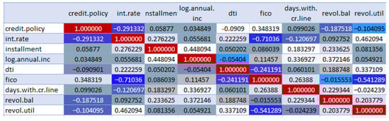
Figure 2. Correlation between the features.

A histogram of two FICO distributions, one for each credit policy outcome, is shown in Figure 3. Figure 4 is the same as Figure 3, except that the not fully paid column is selected. Figure 5 depicts a seaborn countplot of loans by purpose, and the not fully paid column is colored.

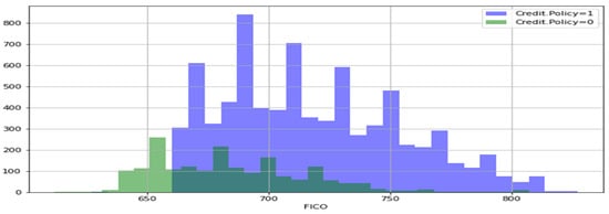
Figure 3. Credit-policy histogram.

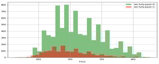
Figure 4. Not-fully-paid histogram.

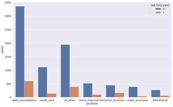
Figure 5. Counts of loans by purpose.

In Figure 6, we created the trend between FICO score and interest rate to check the co-relation between the two. In Figure 7, we created the lmplots to see if the trend differs between not fully paid and credit policy.

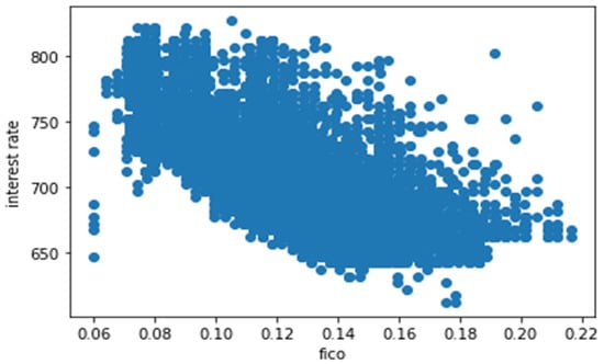
Figure 6. Correlation between FICO score and interest rate.

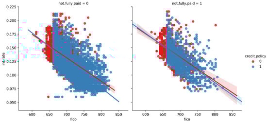
Figure 7. Trend between not fully paid and credit policy.

From Figure 7, we can observe the trend between not fully paid and credit policy. In the first histogram, there is a relationship between interest rate and fico, i.e., the credit score of the borrowers who are not going to pay the loan completely, while in the second histogram, there is a relationship between interest rate and FICO, i.e., the credit score of the borrowers who are going to pay the loan completely. Blue dots show the customers who meet the credit underwriting criteria, while red dots show the customers who do not meet the credit underwriting criteria of the LendingClub.com. After analyzing the features of the datasets, we split the datasets into training and testing data using sklearn in the ratio of 70:30, respectively. The holdout validation strategy was implemented for splitting the datasets into training and testing. In the holdout validation strategy, when dealing with large datasets, the typical split is 70:30, whereas for smaller datasets, the split can be as high as 90:10. In our research, we used a large dataset for fraud prediction; thus, we adopted the 70:30 ratio. We originally had 9578 data entries before the splitting of the data. Thus, 30% of 9578 is 2874, meaning that the remaining 70% of the original data was used for the training of the data, i.e., 6704 entries of the loan data. Then, we applied all the six major classification models on the training and testing set of the data, which were already split [76,77,78,79,80,81]. Firstly, we created an instance for each model and fit it to the training data. Then, we conducted a prediction from the test set and evaluated the classification report, confusion matrix, and accuracy score. Our major objective was to lower the false positive (FPR) parameter of each model’s confusion matrix, as illustrated in Table 5 and Table 6.

Table 5. Classification report of NB, DT, and KNN models.

Measure	NB	DT	KNN
Sensitivity	0.84	0.84	0.83
Specificity	0.36	0.2	0.17
Precision	0.96	0.83	0.96
NPV	0.09	0.21	0.03
FPR	0.63	0.79	0.82
FDR	0.03	0.16	0.03
FNR	0.15	0.15	0.16
Accuracy	0.82	0.73	0.81
F1 Score	0.9	0.83	0.89

Table 6. Classification report of RF, SVM, and LR models.

Measure	RF	SVM	LR
Sensitivity	0.83	0.83	0.83
Specificity	0.5	-	0.36
Precision	0.99	1	0.99
NPV	0.02	0	0
FPR	0.5	-	0.63
FDR	0.004	0	0
FNR	0.16	0.16	0.16
Accuracy	0.83	0.83	0.83
F1 Score	0.9	0.9	0.9

In Table 5 and Table 6, the FPR for NB is 0.63, DT gave the NPR as 0.79, KNN as 0.82, and RF as 0.5. We note here that KNN gave a very good accuracy, but FPR was also high. Here, NB gave optimal results, although other algorithm accuracies were comparable. We can also see that the F1 score of all algorithms were almost the same, but the detail analysis was very important in the case of financial fraud detection. It even become crucial when we have very little data or we do not have the class imbalance dataset.

In Figure 8a,b, the features we took into account are credit policy, log annual increment, days with credit line, interest rate, installment, dti, FICO score, revolving balance, revolving line utilization rate, etc. As we can see, there is a negative correlation between the FICO score and interest; other features did not show any trends, making it more difficult to train the model, and we need a more sophisticated algorithm to deep dive into the dataset.

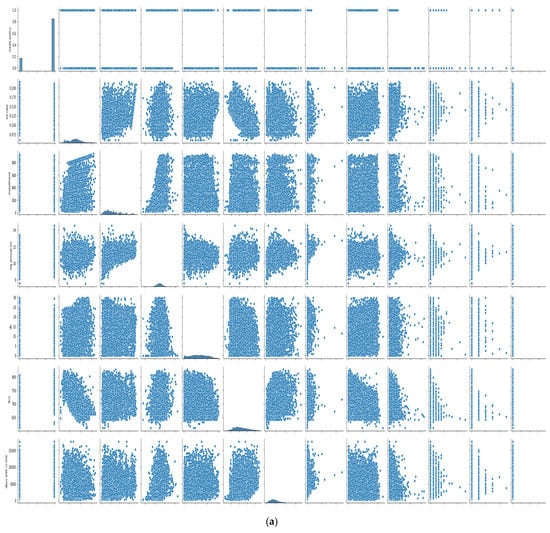
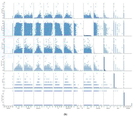
Figure 8. (a) Cross plot of dataset features. (b) Cross plot of dataset features.

There are classification results via CM obtained separately for each algorithm. Figure 9 shows the CM for the NB model, Figure 10 shows the CM for the DT model, Figure 11 shows the CM for the KNN model, Figure 12 shows the CM for the RF model, Figure 13 shows the CM for the SVM model, and Figure 14 shows the CM for the LR model.

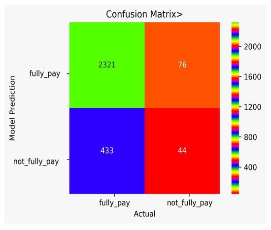
Figure 9. CM for the NB model.

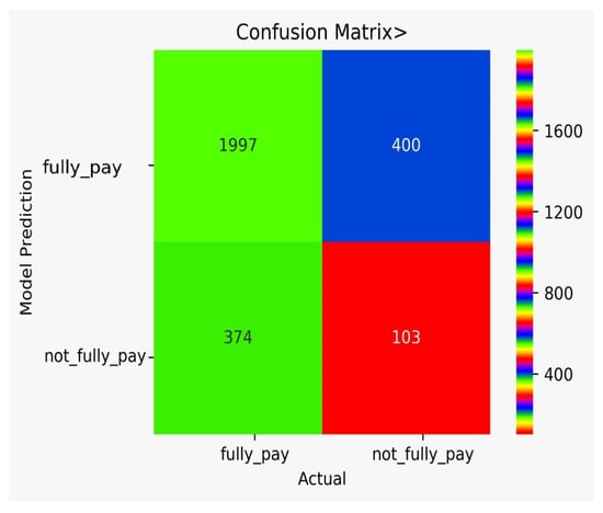
Figure 10. CM for the DT model.

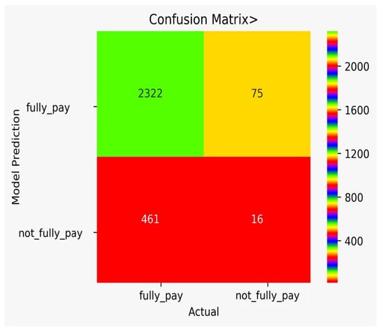
Figure 11. CM for the KNN model.

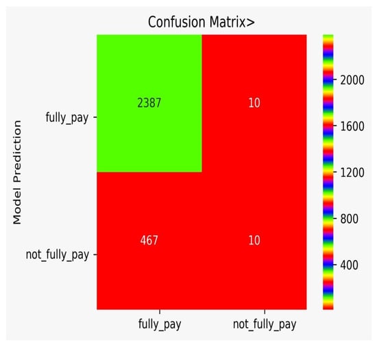
Figure 12. CM for the RF model.

Figure 13. CM for the SVM model.

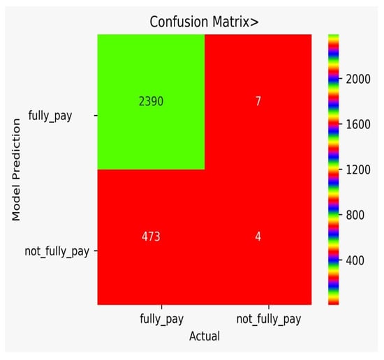
Figure 14. CM for the LR model.

In Table 7, the comparison of different models is shown. The FP for DT is very high, while the FP for SVM is zero. However, we need to think of not only accuracy, but rather a varying number of misclassification rates that force us to use multiple algorithms and to conduct a detail analysis, as we performed in our work. It can be observed from Table 7 that the adopted approach performed better in the prediction of the possibility of bank fraud than the other approaches, which can observed by looking at its accuracy score, f-score, CAP curve, and false-positive parameter.

Table 7. Comparison of different models.

Classification Algorithms	Accuracy	FP	FN	F-Score
				0	1
DT	72.89%	407	372	0.84	0.21
NB	82.28%	76	433	0.9	0.15
RF	83.33%	9	470	0.91	0.03
KNN	81.35%	75	461	0.9	0.06
LR	83.47%	2	473	0.9	0.06
SVM	83.40%	0	477	0.91	0

Figure 15 shows the CAP curve analysis. We conducted a CAP curve analysis to visualize the discriminative power of the models, which means the model with the larger area covered by the CAP curve between the random model (dotted line) and the perfect model (blue line) is the best model [84,85,86,87]. We applied all the six major classification models on the training and testing set of the data, which were already split. Firstly, we created an instance for each model and fit it into the training data. Then, we conducted a prediction from the test set and evaluated the classification report, confusion matrix, and accuracy score.

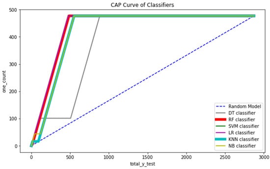
Figure 15. CAP curve analysis of all the classifiers.

5. Conclusions

The following in-depth descriptions are based on the analyses undertaken. To begin, we compared the ML-based models to the current empirical models and found that, while the latter only accounted for application factors, the former also accounted for the behavioral ones. After that, the study compared the six ML approaches using sensitivity, specificity, accuracy, precision, F1 score, and CAP curve tests, and it concluded that the SVM model delivered the best results in the great model of the life cycle. Finally, this study’s completion provides new angles for research that will have an effect on credit and credit risk models in the future.

It is possible for financial institutions to assess whether or not a customer is engaging in fraudulent activity by incorporating this paper’s model into their existing systems. If financial institutions take these precautions, they will increase their odds of warding off future cons and fraudulent activity.

In any area of study, the importance of comprehending human behavior in the present setting has grown. Knowing how the impacts associated with the behavior of a system, an economic unit, or any other actor in a system affects either the micro or macro level and is, thus, a topic of great interest. The year 2020 has been forecasted to be a challenging one for Romanian banks, as reported in 2019 [87]. In fact, according to government predictions, as many as 12% of banks could post losses in the current fiscal year, with the profitability per customer down by around 60% from 2019 levels. Most financial institutions are conducting internal and external research to learn more about their clients’ wants and needs, but many questions remain. Business banks place a premium on maintaining long-term relationships with their clientele; as such, they view customer behavior analysis as a crucial part of any study, as it helps them predict their clients’ reactions and shape the design of the products and services they provide.

Due to the competitive environment in which banks operate, a priority must be placed on satisfying the needs of present customers in order to keep them as clients. Another objective of banks is to keep their loan portfolios in good shape. This study shows that these problems can be solved by employing machine learning methods.

6. Future Directions

In data gathering, we can collect user’s social media history and tweets to find sentiments and fuzziness [23,72] for fraud prediction. The data gathered may be big enough to process using big data analytics to obtain a real time alert [24,71].

As a weapon for combating financial fraud and corruption, forensic accounting should be mandated in deposit money institutions in order to enhance company performance via the application of fraud detection techniques in forensic accounting.

Further studies are needed in the area of financial fraud to analyze the accuracy of various methods for minimizing financial fraud as well as the flaws and biases of the utilized methodology in terms of their application to identify and prevent fraud. More studies on work requirements and task rotation are recommended for an auditor to be productive. Concerning technological fraud, research should focus on the importance of technology training, employee cybersecurity education, and the limits of organizational capacities, structure, legal restrictions, and technical assistance. Future research on white-collar crime should focus on contemporary multi-level audit programmers and realistic account measurement standards, defining white-collar crime by measuring the degree and types of crime, organizations, fraud context, and other criminal features in order to reduce top-level fraud.

References

- DaCorte, A.M. The Effects of the Internet on Financial Institutions’ Fraud Mitigation. Ph.D. Thesis, Utica University, Utica, NY, USA, 2022. [Google Scholar]
- Li, Y. Credit risk prediction based on machine learning methods. In Proceedings of the 2019 14th International Conference on Computer Science & Education (ICCSE), Toronto, ON, Canada, 19–21 August 2019; pp. 1011–1013. [Google Scholar]
- Zhu, L.; Qiu, D.; Ergu, D.; Ying, C.; Liu, K. A study on predicting loan default based on the random forest algorithm. Procedia Comput. Sci. 2019, 162, 503–513. [Google Scholar] [CrossRef]
- Vojtek, M.; Koèenda, E. Credit-Scoring methods. Czech J. Econ. Financ. (Financ. A Uver) 2006, 56, 152–167. [Google Scholar]
- Arora, B. A Review of Credit Card Fraud Detection Techniques. Recent Innov. Comput. 2022, 832, 485–496. [Google Scholar] [CrossRef]
- Rehman, A.U.; Jiang, A.; Rehman, A.; Paul, A. Weighted Based Trustworthiness Ranking in Social Internet of Things by using Soft Set Theory. In Proceedings of the 2019 IEEE 5th International Conference on Computer and Communications (ICCC), Chengdu, China, 6–9 December 2019; pp. 1644–1648. [Google Scholar] [CrossRef]
- Ghatasheh, N. Business Analytics using Random Forest Trees for Credit Risk Prediction: A Comparison Study. Int. J. Adv. Sci. Technol. 2014, 72, 19–30. [Google Scholar] [CrossRef]
- Breeden, J.L. A survey of machine learning in credit risk. J. Crédit. Risk 2021, 17, 1–62. [Google Scholar] [CrossRef]
- Madaan, M.; Kumar, A.; Keshri, C.; Jain, R.; Nagrath, P. Loan default prediction using decision trees and random forest: A comparative study. IOP Conf. Series: Mater. Sci. Eng. 2021, 1022, 012042. [Google Scholar] [CrossRef]
- Pidikiti, S.; Myneedi, P.; Nagarapu, S.; Namburi, V.K.; Vikas, K. Loan prediction by using machine learning models. Int. J. Eng. Tech. 2019, 5, 144–148. [Google Scholar]
- Vorobyev, I.; Krivitskaya, A. Reducing False Positives in Bank Anti-fraud Systems Based on Rule Induction in Distributed Tree-based Models. Comput. Secur. 2022, 120, 102786. [Google Scholar] [CrossRef]
- Islam, U.; Muhammad, A.; Mansoor, R.; Hossain, S.; Ahmad, I.; Eldin, E.T.; Khan, J.A.; Rehman, A.U.; Shafiq, M. Detection of Distributed Denial of Service (DDoS) Attacks in IOT Based Monitoring System of Banking Sector Using Machine Learning Models. Sustainability 2022, 14, 8374. [Google Scholar] [CrossRef]
- Onyema, E.M.; Kumar, M.A.; Balasubaramanian, S.; Bharany, S.; Rehman, A.U.; Eldin, E.T.; Shafiq, M. A Security Policy Protocol for Detection and Prevention of Internet Control Message Protocol Attacks in Software Defined Networks. Sustainability 2022, 14, 11950. [Google Scholar] [CrossRef]
- Jency, X.F.; Sumathi, V.P.; Sri, J.S. An exploratory data analysis for loan prediction based on nature of the clients. Int. J. Recent Technol. Eng. (IJRTE) 2018, 7, 176–179. [Google Scholar]
- Berrada, I.R.; Barramou, F.Z.; Alami, O.B. A review of Artificial Intelligence approach for credit risk assessment. In Proceedings of the 2022 2nd International Conference on Artificial Intelligence and Signal Processing (AISP), Vijayawada, India, 12–14 February 2022. [Google Scholar]
- Addo, P.M.; Guegan, D.; Hassani, B. Credit Risk Analysis Using Machine and Deep Learning Models. Risks 2018, 6, 38. [Google Scholar] [CrossRef]
- Hamid, A.J.; Ahmed, T.M. Developing prediction model of loan risk in banks using data mining. Mach. Learn. Appl. Int. J. (MLAIJ) 2016, 3, 1–9. [Google Scholar]
- Mazhar, M.S.; Saleem, Y.; Almogren, A.; Arshad, J.; Jaffery, M.H.; Rehman, A.U.; Shafiq, M.; Hamam, H. Forensic Analysis on Internet of Things (IoT) Device Using Machine-to-Machine (M2M) Framework. Electronics 2022, 11, 1126. [Google Scholar] [CrossRef]
- Rehman, A.U.; Tariq, R.; Rehman, A.; Paul, A. Collapse of Online Social Networks: Structural Evaluation, Open Challenges, and Proposed Solutions. In Proceedings of the 2020 IEEE Globecom Workshops (GC Wkshps), Taipei, Taiwan, 7–11 December 2020; pp. 1–6. [Google Scholar] [CrossRef]
- Agarwal, P.; Ahmed, R.; Ahmad, T. Identification and ranking of key persons in a Social Networking Website using Hadoop & Big Data Analytics. In Proceedings of the International Conference on Advances in Information Communication Technology & Computing, Bikaner, India, 12–13 August 2016; pp. 1–6. [Google Scholar] [CrossRef]
- Singh, B.; Kumar, K.; Mohan, S.; Ahmad, R. Ensemble of Clustering Approaches for Feature Selection of High Dimensional Data. In Proceedings of the 2nd International Conference on Advance Computing and Software Engineering, ICACSE-2019, Sultanpur, India, 8–9 February 2019. [Google Scholar]
- Choi, H.; Jang, E.; Alemi, A.A. WAIC, but Why? Generative Ensembles for Robust Anomaly Detection. arXiv 2019, arXiv:1810.01392. Available online: https://arxiv.org/abs/1810.01392 (accessed on 21 July 2022).
- Ahmed, R.; Tanvir, A. Fuzzy concept map generation from academic data sources. In Applications of Artificial Intelligence Techniques in Engineering; Springer: Singapore, 2019; pp. 415–424. [Google Scholar]
- Shah, S.A.A.; Ahammad, N.A.; El Din, E.M.T.; Gamaoun, F.; Awan, A.U.; Ali, B. Bio-Convection Effects on Prandtl Hybrid Nanofluid Flow with Chemical Reaction and Motile Microorganism over a Stretching Sheet. Nanomaterials 2022, 12, 2174. [Google Scholar] [CrossRef]
- Nguyen, N.; Duong, T.; Chau, T.; Nguyen, V.-H.; Trinh, T.; Tran, D.; Ho, T. A Proposed Model for Card Fraud Detection Based on CatBoost and Deep Neural Network. IEEE Access 2022, 10, 96852–96861. [Google Scholar] [CrossRef]
- Bolton, R.J.; Hand, D.J. Statistical Fraud Detection: A Review. Stat. Sci. 2002, 17, 235–255. [Google Scholar] [CrossRef]
- Weston, D.J.; Hand, D.; Adams, N.M.; Whitrow, C.; Juszczak, P. Plastic card fraud detection using peer group analysis. Adv. Data Anal. Classif. 2008, 2, 45–62. [Google Scholar] [CrossRef]
- Duman, E.; Ozcelik, M.H. Detecting credit card fraud by genetic algorithm and scatter search. Expert Syst. Appl. 2011, 38, 13057–13063. [Google Scholar] [CrossRef]
- Ramakalyani, K.; Umadevi, D. Fraud detection of credit card payment system by genetic algorithm. Int. J. Sci. Eng. Res. 2012, 3, 1–6. [Google Scholar]
- Bentley, P.J.; Kim, J.; Jung, G.-H.; Choi, J.-U. Fuzzy Darwinian Detection of Credit Card Fraud. Available online: https://www.researchgate.net/publication/228971658_Fuzzy_Darwinian_detection_of_credit_card_fraud (accessed on 14 October 2022).
- Chouiekh, A.; Haj, E.H.I.E. ConvNets for Fraud Detection analysis. Procedia Comput. Sci. 2018, 127, 133–138. [Google Scholar] [CrossRef]
- Zhang, Z.; Zhou, X.; Zhang, X.; Wang, L.; Wang, P. A Model Based on Convolutional Neural Network for Online Transaction Fraud Detection. Secur. Commun. Networks 2018, 2018, 5680264. [Google Scholar] [CrossRef]
- Kazemi, Z.; Zarrabi, H. Using deep networks for fraud detection in the credit card transactions. In Proceedings of the 2017 IEEE 4th International Conference on Knowledge-Based Engineering and Innovation (KBEI), Tehran, Iran, 22 December 2017. [Google Scholar]
- Schreyer, M.; Sattarov, T.; Borth, D.; Dengel, A.; Reimer, B. Detection of Anomalies in Large Scale Accounting Data Using Deep Autoencoder Networks. Available online: https://arxiv.org/abs/1709.05254 (accessed on 14 October 2022).
- Renström, M.; Holmsten, T. Fraud Detection on Unlabeled Data with Unsupervised Machine Learning. 2018. Available online: https://kth.diva-portal.org/ (accessed on 17 June 2021).
- Srivastava, A.; Kundu, A.; Sural, S.; Majumdar, A. Credit Card Fraud Detection Using Hidden Markov Model. IEEE Trans. Dependable Secur. Comput. 2008, 5, 37–48. [Google Scholar] [CrossRef]
- Esakkiraj, S.; Chidambaram, S. A predictive approach for fraud detection using hidden Markov model. Int. J. Eng. Res. Technol. 2013, 2, 1–7. [Google Scholar]
- Mishra, J.S.; Panda, S.; Mishra, A.K. A novel approach for credit card fraud detection targeting the Indian market. Int. J. Comput. Sci. 2013, 10, 172–179. [Google Scholar]
- Brabazon, A.; Cahill, J.; Keenan, P.; Walsh, D. Identifying online credit card fraud using Artificial Immune Systems. In Proceedings of the Congress on Evolutionary Computation, Barcelona, Spain, 18–23 July 2010; pp. 1–7. [Google Scholar] [CrossRef]
- Wong, N.; Ray, P.; Stephens, G.; Lewis, L. Artificial immune systems for the detection of credit card fraud: An architecture, prototype and preliminary results. Inf. Syst. 2012, 22, 53–76. [Google Scholar] [CrossRef]
- Sánchez, D.; Vila, M.A.; Cerda, L.; Serrano, J.M. Association rules applied to credit card fraud detection. Expert Syst. Appl. 2009, 36, 3630–3640. [Google Scholar] [CrossRef]
- Sahin, Y.; Bulkan, S.; Duman, E. A cost-sensitive decision tree approach for fraud detection. Expert Syst. Appl. 2013, 40, 5916–5923. [Google Scholar] [CrossRef]
- Bahnsen, A.C.; Stojanovic, A.; Aouada, D.; Ottersten, B. Cost Sensitive Credit Card Fraud Detection Using Bayes Minimum Risk. In Proceedings of the 2013 12th International Conference on Machine Learning and Applications, Miami, FL, USA, 4–7 December 2013; 2013; Volume 1, pp. 333–338. [Google Scholar] [CrossRef]
- Roseline, J.F.; Naidu, G.; Pandi, V.S.; Rajasree, S.A.A.; Mageswari, N. Autonomous credit card fraud detection using machine learning approach. Comput. Electr. Eng. 2022, 102, 108132. [Google Scholar] [CrossRef]
- Ganji, V.R.; Mannem, S.N.P. Credit card fraud detection using antik nearest neighbor algorithm. Int. J. Comput. Sci. Eng. 2012, 4, 1035–1039. [Google Scholar]
- Hormozi, H.; Akbari, M.K.; Hormozi, E.; Javan, M.S. Credit cards fraud detection by negative selection algorithm on hadoop (To reduce the training time). In Proceedings of the 5th Conference on Information and Knowledge Technology, Shiraz, Iran, 28–30 May 2013; pp. 40–43. [Google Scholar] [CrossRef]
- Quah, J.T.S.; Sriganesh, M. Real-Time credit card fraud detection using computational intelligence. Expert Syst. Appl. 2008, 35, 2007–2009. [Google Scholar] [CrossRef]
- Kundu, A.; Panigrahi, S.; Sural, S.; Majumdar, A.K. BLAST-SSAHA Hybridization for Credit Card Fraud Detection. IEEE Trans. Dependable Secur. Comput. 2009, 6, 309–315. [Google Scholar] [CrossRef]
- Sherly, K.K.; Nedunchezhian, R. BOAT adaptive credit card fraud detection system. In Proceedings of the 2010 IEEE International Conference on Computational Intelligence and Computing Research, Coimbatore, India, 28–29 December 2010; pp. 1–7. [Google Scholar] [CrossRef]
- Minegishi, T.; Niimi, A. Detection of fraud use of credit card by extended VFDT. In Proceedings of the World Congress on Internet Security (WorldCIS-2011), London, UK, 21–23 February 2011; pp. 152–159. [Google Scholar] [CrossRef]
- Bharany, S.; Sharma, S.; Frnda, J.; Shuaib, M.; Khalid, M.I.; Hussain, S.; Iqbal, J.; Ullah, S.S. Wildfire Monitoring Based on Energy Efficient Clustering Approach for FANETS. Drones 2022, 6, 193. [Google Scholar] [CrossRef]
- Ghosh, S.; Reilly, D.L. Credit card fraud detection with a neural-network. In Proceedings of the Twenty-Seventh Hawaii International Conference on System Sciences, Wailea, HI, USA, 4–7 January 1994; Volume 3, pp. 621–630. [Google Scholar] [CrossRef]
- Zaslavsky, V.; Strizhak, A. Credit Card Fraud Detection Using Self-Organizing Maps. Inf. Secur. Int. J. 2006, 18, 48–63. [Google Scholar] [CrossRef]
- Ogwueleka, F.N. Data mining application in credit card fraud detection system. J. Eng. Sci. Technol. 2011, 6, 311–322. [Google Scholar]
- Patidar, R.; Sharma, L. Credit card fraud detection using neural network. Int. J. Soft Comput. Eng. 2011, 1, 32–38. [Google Scholar]
- Syeda, M.; Zhang, Y.-Q.; Pan, Y. Parallel granular neural networks for fast credit card fraud detection. In Proceedings of the 2002 IEEE World Congress on Computational Intelligence, 2002 IEEE International Conference on Fuzzy Systems, FUZZ-IEEE’02, Cat. No. 02CH37291, Atlanta, GA, USA, 12–17 May 2002; pp. 572–577. [Google Scholar] [CrossRef]
- Maes, S.; Tuyls, K.; Vanschoenwinkel, B.; Manderick, B. Credit card fraud detection using Bayesian and neural networks. In Proceedings of the 1st International Naiso Congress on Neuro Fuzzy Technologies, Havana, Cuba, 16–19 January 2002; pp. 261–270. [Google Scholar]
- Whitrow, C.; Hand, D.; Juszczak, P.; Weston, D.J.; Adams, N.M. Transaction aggregation as a strategy for credit card fraud detection. Data Min. Knowl. Discov. 2008, 18, 30–55. [Google Scholar] [CrossRef]
- Bhattacharyya, S.; Jha, S.; Tharakunnel, K.; Westland, J.C. Data mining for credit card fraud: A comparative study. Decis. Support Syst. 2011, 50, 602–613. [Google Scholar] [CrossRef]
- Subashini, B.; Chitra, K. Enhanced system for revealing fraudulence in credit card approval. Int. J. Eng. Res. Technol. 2013, 2, 936–949. [Google Scholar]
- Mahmoudi, N.; Duman, E. Detecting credit card fraud by Modified Fisher Discriminant Analysis. Expert Syst. Appl. 2015, 42, 2510–2516. [Google Scholar] [CrossRef]
- Sailusha, R.; Gnaneswar, V.; Ramesh, R.; Rao, G.R. Credit Card Fraud Detection Using Machine Learning. In Proceedings of the 2020 4th International Conference on Intelligent Computing and Control Systems (ICICCS), Madurai, India, 13–15 May 2020; pp. 1264–1270. [Google Scholar] [CrossRef]
- Padmaja, T.M.; Dhulipalla, N.; Bapi, R.S.; Krishna, P.R. Unbalanced data classification using extreme outlier elimination and sampling techniques for fraud detection. In Proceedings of the 15th International Conference on Advanced Computing and Communications (ADCOM 2007), Guwahati, India, 18–21 December 2007; pp. 511–516. [Google Scholar]
- Bharany, S.; Sharma, S.; Khalaf, O.I.; Abdulsahib, G.M.; Al Humaimeedy, A.S.; Aldhyani, T.H.H.; Maashi, M.; Alkahtani, H. A Systematic Survey on Energy-Efficient Techniques in Sustainable Cloud Computing. Sustainability 2022, 14, 6256. [Google Scholar] [CrossRef]
- Pumsirirat, A.; Yan, L. Credit Card Fraud Detection using Deep Learning based on Auto-Encoder and Restricted Boltzmann Machine. Int. J. Adv. Comput. Sci. Appl. 2018, 9, 18–25. [Google Scholar] [CrossRef]
- Bharany, S.; Kaur, K.; Badotra, S.; Rani, S.; Kavita; Wozniak, M.; Shafi, J.; Ijaz, M.F. Efficient Middleware for the Portability of PaaS Services Consuming Applications among Heterogeneous Clouds. Sensors 2022, 22, 5013. [Google Scholar] [CrossRef]
- Jurgovsky, J.; Granitzer, M.; Ziegler, K.; Calabretto, S.; Portier, P.-E.; He-Guelton, L.; Caelen, O. Sequence classification for credit-card fraud detection. Expert Syst. Appl. 2018, 100, 234–245. [Google Scholar] [CrossRef]
- Fiore, U.; De Santis, A.; Perla, F.; Zanetti, P.; Palmieri, F. Using generative adversarial networks for improving classification effectiveness in credit card fraud detection. Inf. Sci. 2019, 479, 448–455. [Google Scholar] [CrossRef]
- Bharany, S.; Badotra, S.; Sharma, S.; Rani, S.; Alazab, M.; Jhaveri, R.H.; Gadekallu, T.R. Energy efficient fault tolerance techniques in green cloud computing: A systematic survey and taxonomy. Sustain. Energy Technol. Assess. 2022, 53, 102613. [Google Scholar] [CrossRef]
- Gupta, A.; Lohani, M.C. Comparative Analysis of Numerous Approaches in Machine Learning to Predict Financial Fraud in Big Data Framework; Springer: Singapore, 2021; pp. 107–123. [Google Scholar] [CrossRef]
- Mao, X.; Sun, H.; Zhu, X.; Li, J. Financial fraud detection using the related-party transaction knowledge graph. Procedia Comput. Sci. 2022, 199, 733–740. [Google Scholar] [CrossRef]
- Lu, Y. Deep Neural Networks and Fraud Detection. DIVA. 2017. Available online: http://uu.divaportal.org/smash/record.jsf?pid=diva2%3A1150344&dswid=-3078 (accessed on 15 August 2022).
- Gómez, J.A.; Arévalo, J.; Paredes, R.; Nin, J. End-to-end neural network architecture for fraud scoring in card payments. Pattern Recognit. Lett. 2018, 105, 175–181. [Google Scholar] [CrossRef]
- Wang, C.; Wang, Y.; Ye, Z.; Yan, L.; Cai, W.; Pan, S. Credit Card Fraud Detection Based on Whale Algorithm Optimized BP Neural Network. In Proceedings of the 2018 13th International Conference on Computer Science & Education (ICCSE), Colombo, Sri Lanka, 8–11 August 2018; pp. 1–4. [Google Scholar] [CrossRef]
- Abroyan, N. Neural Networks for Financial Market Risk Classification. Front. Signal Process. 2017, 1, 62–66. [Google Scholar] [CrossRef]
- Rehman, A.U.; Naqvi, R.A.; Rehman, A.; Paul, A.; Sadiq, M.T.; Hussain, D. A Trustworthy SIoT Aware Mechanism as an Enabler for Citizen Services in Smart Cities. Electronics 2020, 9, 918. [Google Scholar] [CrossRef]
- Bharany, S.; Sharma, S.; Bhatia, S.; Rahmani, M.K.I.; Shuaib, M.; Lashari, S.A. Energy Efficient Clustering Protocol for FANETS Using Moth Flame Optimization. Sustainability 2022, 14, 6159. [Google Scholar] [CrossRef]
- Rehman, H.U.; Awan, A.U.; Tag-ElDin, E.M.; Alhazmi, S.E.; Yassen, M.F.; Haider, R. Extended hyperbolic function method for the (2 +1)-dimensional nonlinear soliton equation. Results Phys. 2022, 40, 105802. [Google Scholar] [CrossRef]
- Wang, Y.; Wang, W.; Ahmad, I.; Tag-Eldin, E. Multi-Objective Quantum-Inspired Seagull Optimization Algorithm. Electronics 2022, 11, 1834. [Google Scholar] [CrossRef]
- Shaker, Y.O.; Yousri, D.; Osama, A.; Al-Gindy, A.; Tag-Eldin, E.; Allam, D. Optimal Charging/Discharging Decision of Energy Storage Community in Grid-Connected Microgrid Using Multi-Objective Hunger Game Search Optimizer. IEEE Access 2021, 9, 120774–120794. [Google Scholar] [CrossRef]
- Shi, Z.-B.; Yu, T.; Zhao, Q.; Li, Y.; Lan, Y.-B. Comparison of Algorithms for an Electronic Nose in Identifying Liquors. J. Bionic Eng. 2008, 5, 253–257. [Google Scholar] [CrossRef]
- Li, Y.; Li, Z.; Chen, L. Dynamic State Estimation of Generators Under Cyber Attacks. IEEE Access 2019, 7, 125253–125267. [Google Scholar] [CrossRef]
- Kaur, K.; Bharany, S.; Badotra, S.; Aggarwal, K.; Nayyar, A.; Sharma, S. Energy-Efficient polyglot persistence database live migration among heterogeneous clouds. J. Supercomput. 2022, 78, 1–30. [Google Scholar] [CrossRef]
- Srivastava, A.; Ahmed, R.; Singh, P.K.; Shuaib, M.; Alam, T. A Hybrid Approach of Prediction Using Rating and Review Data. Int. J. Inf. Retr. Res. 2022, 12, 1–13. [Google Scholar] [CrossRef]
- Bhatia, S.; Alam, S.; Shuaib, M.; Alhameed, M.H.; Jeribi, F.; Alsuwailem, R.I. Retinal Vessel Extraction via Assisted Multi-Channel Feature Map and U-Net. Front. Public Health 2022, 10, 858327. [Google Scholar] [CrossRef] [PubMed]
- Shuaib, M.; Alam, S.; Ahmed, R.; Qamar, S.; Nasir, M.S.; Alam, M.S. Current Status, Requirements, and Challenges of Blockchain Application in Land Registry. Int. J. Inf. Retr. Res. 2022, 12, 1–20. [Google Scholar] [CrossRef]
- Economia HotNews. Available online: https://economie.hotnews.ro/stiri-finante_banci-24234743-cum-schimbat-pandemia-relatia-banca-marile-necunoscute-ale-bancilor-privire-comportamentul-asteptarile-clientilor.htm (accessed on 10 September 2022).
Publisher’s Note: MDPI stays neutral with regard to jurisdictional claims in published maps and institutional affiliations. |
© 2022 by the authors. Licensee MDPI, Basel, Switzerland. This article is an open access article distributed under the terms and conditions of the Creative Commons Attribution (CC BY) license (https://creativecommons.org/licenses/by/4.0/).