


Influence of Hydraulic Model Complexity on Results of Water Age and Quality Simulation in Municipal Water Supply Systems

 , , , and
Abstract
1. Introduction
2. Methodology
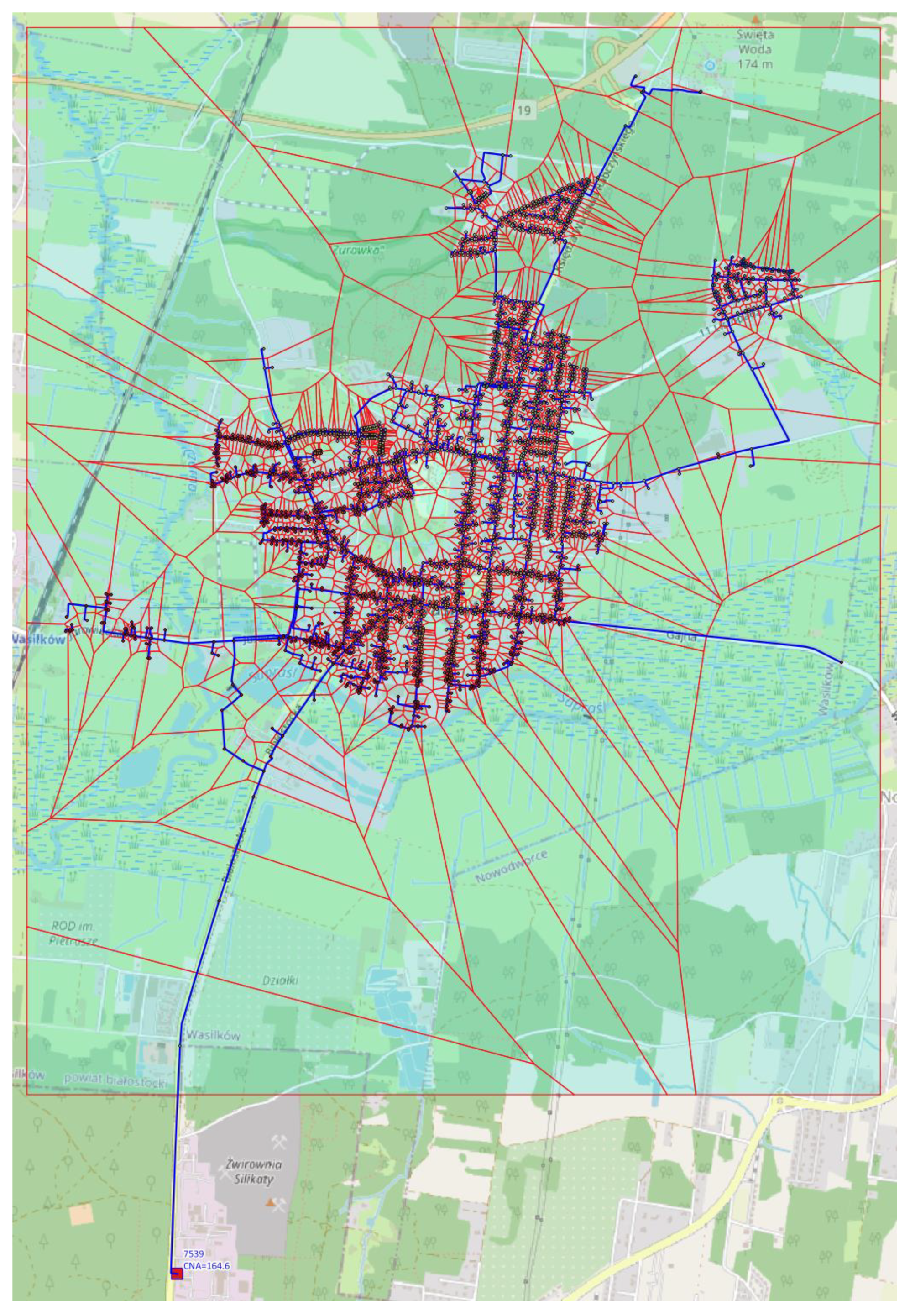
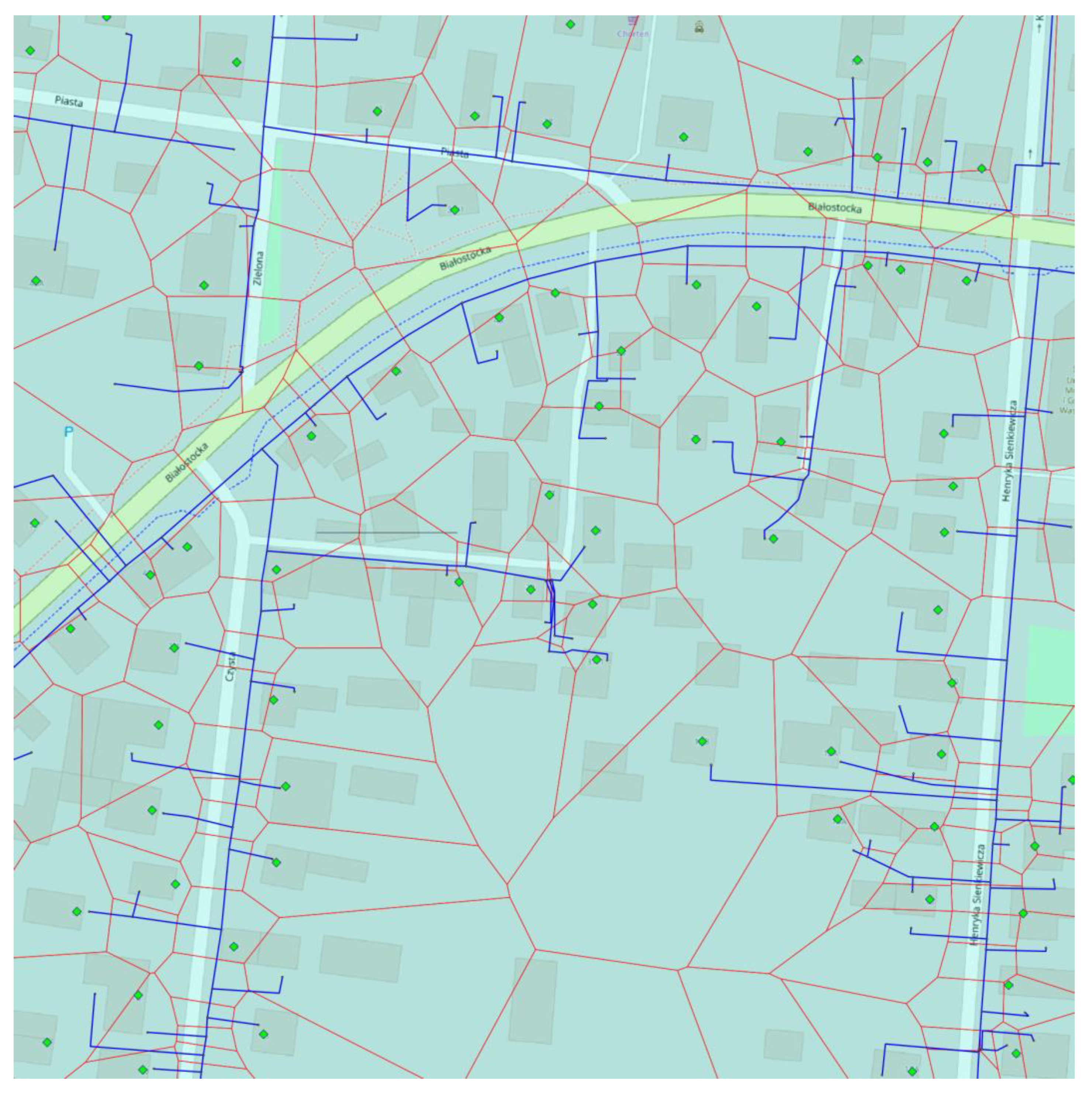
2.1. Complex Model
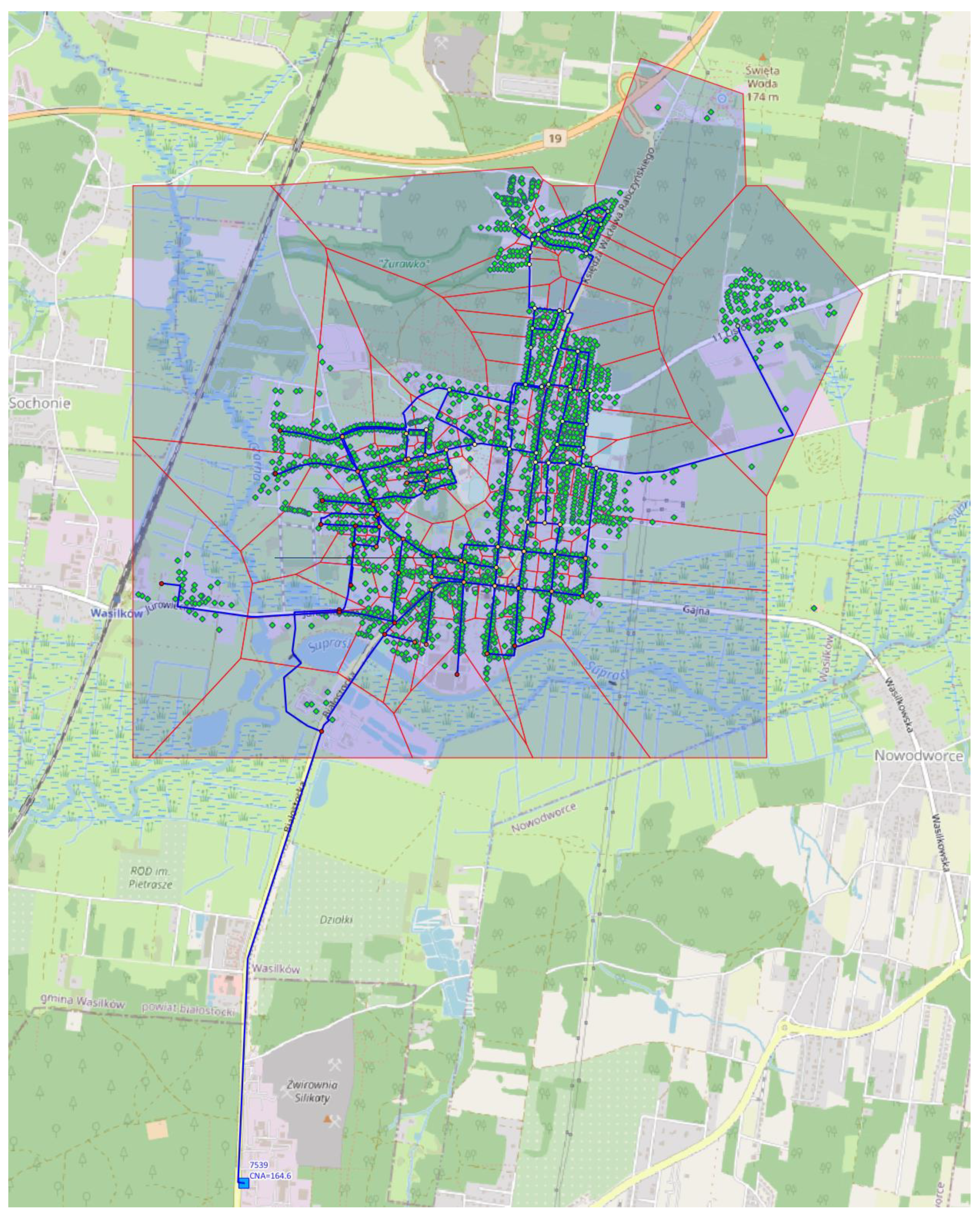
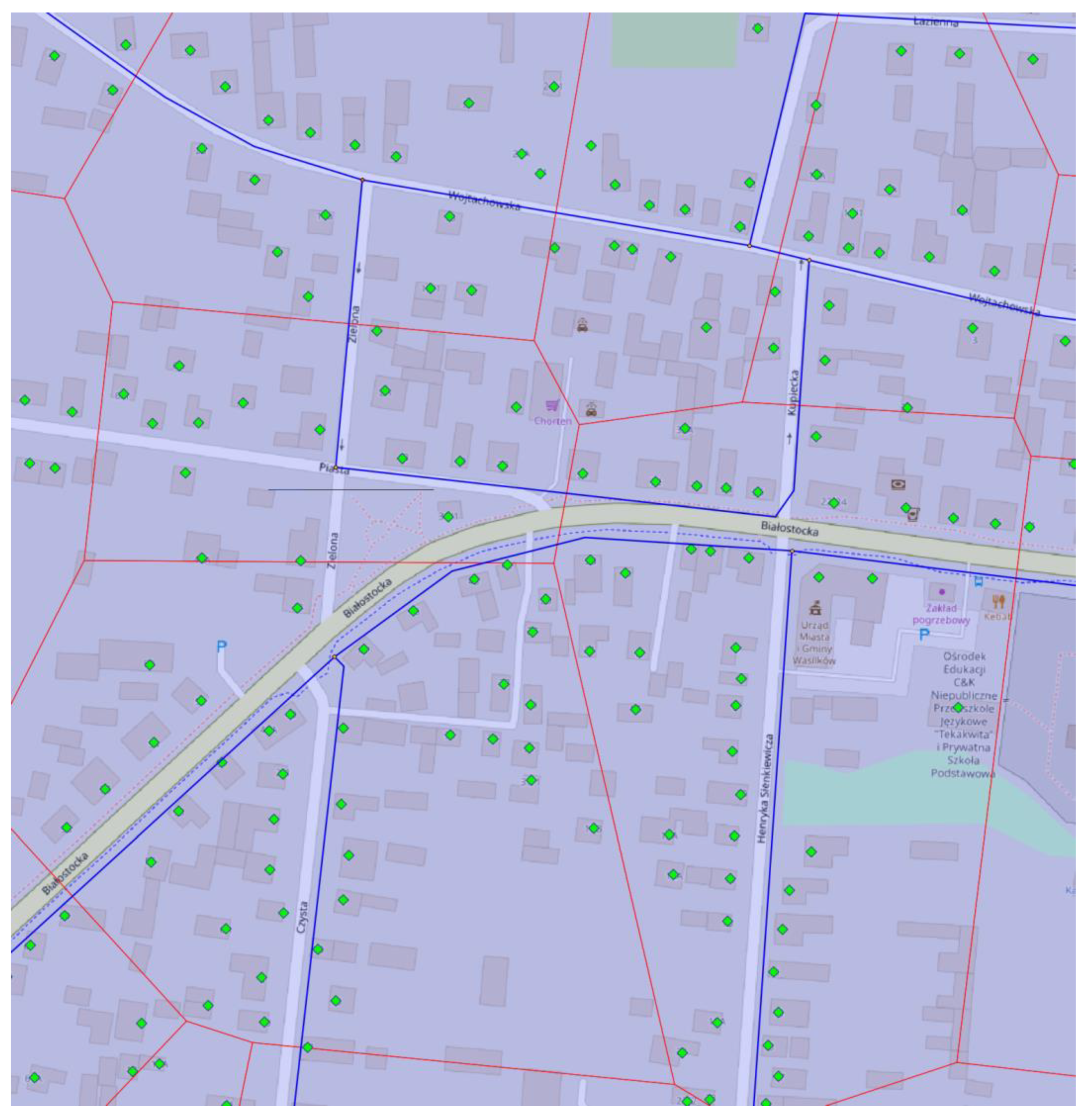
2.2. Simplified Model
3. Results
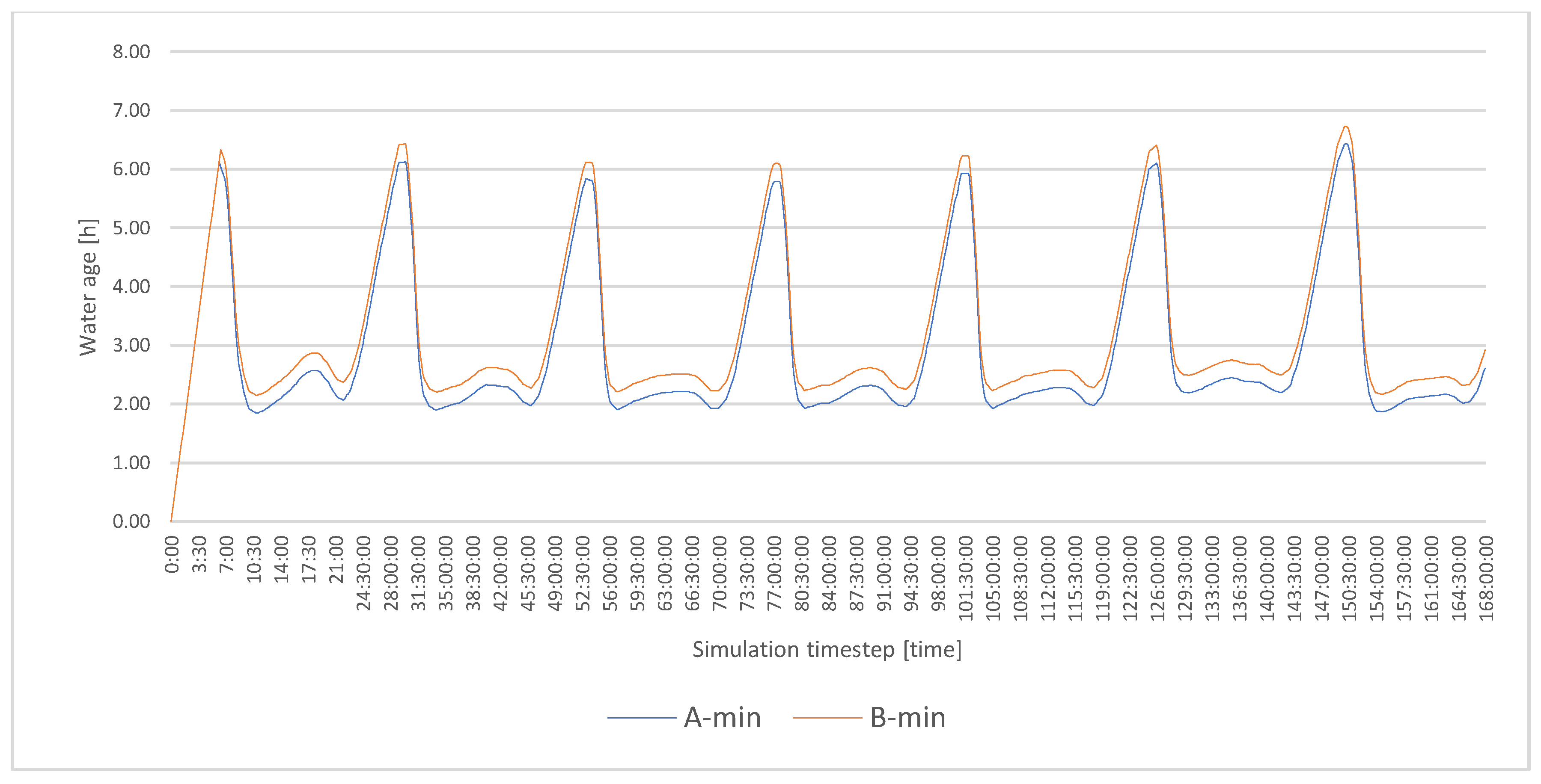
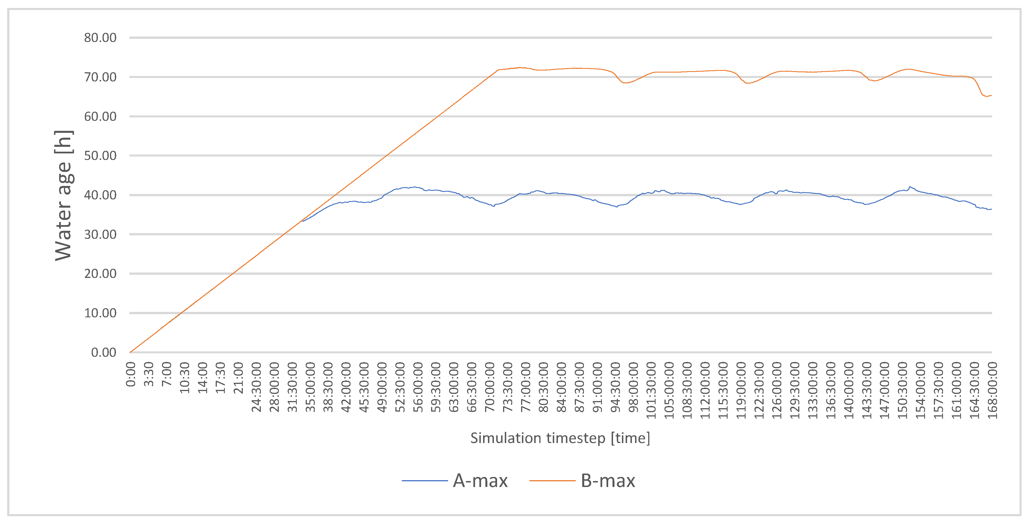
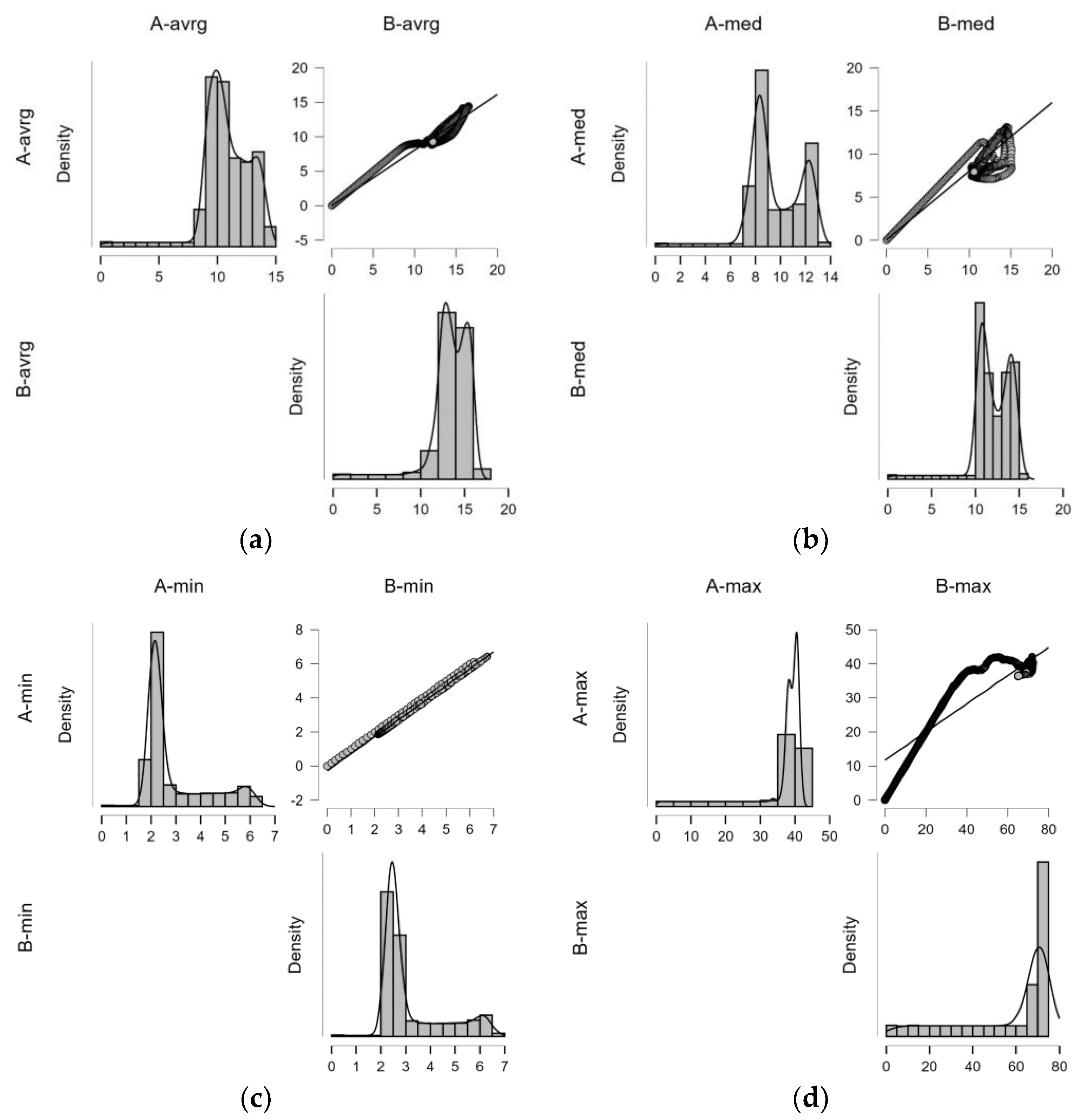
3.1. Descriptive Statistics: Age
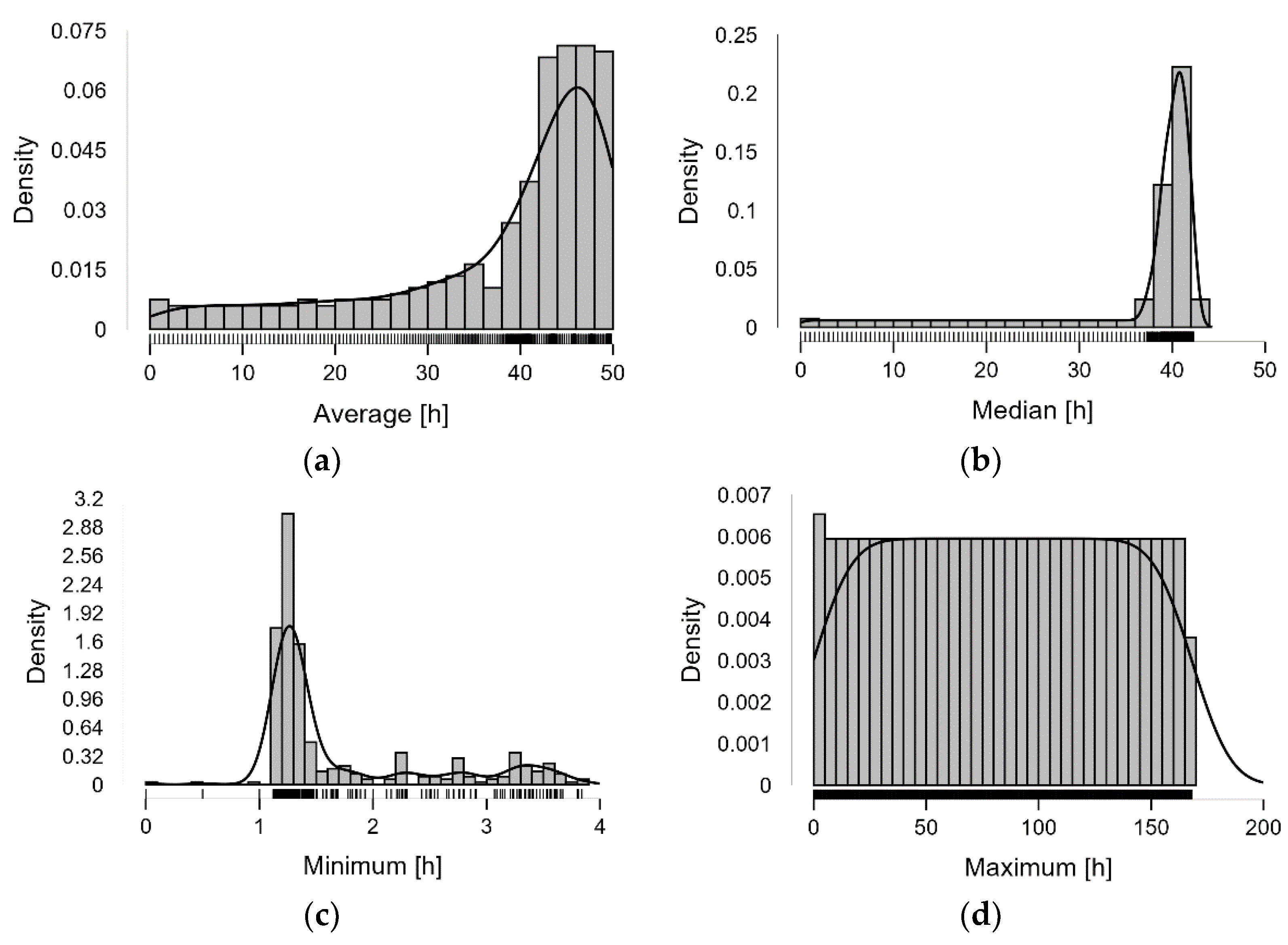
3.2. Descriptive Statistics Complex Model Full Dataset: Age
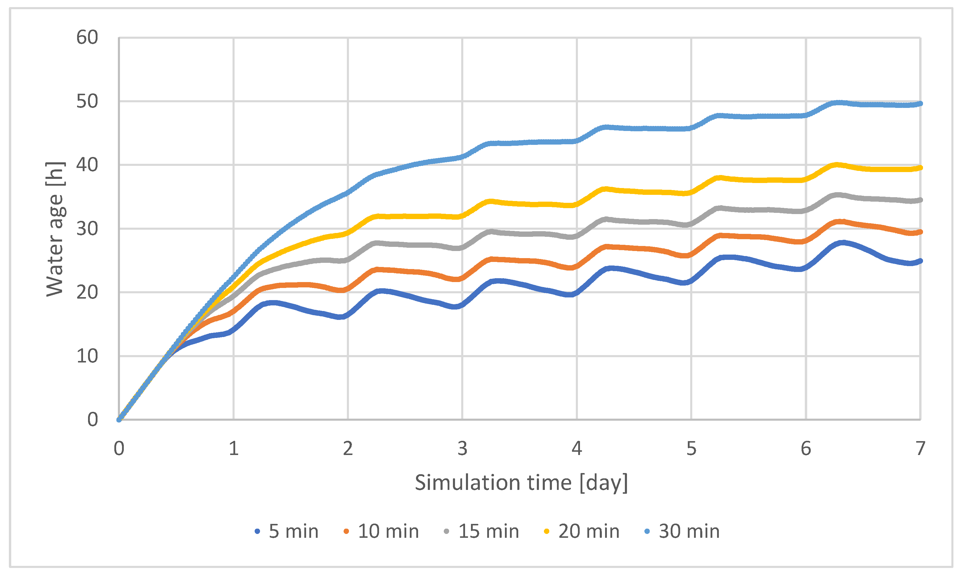
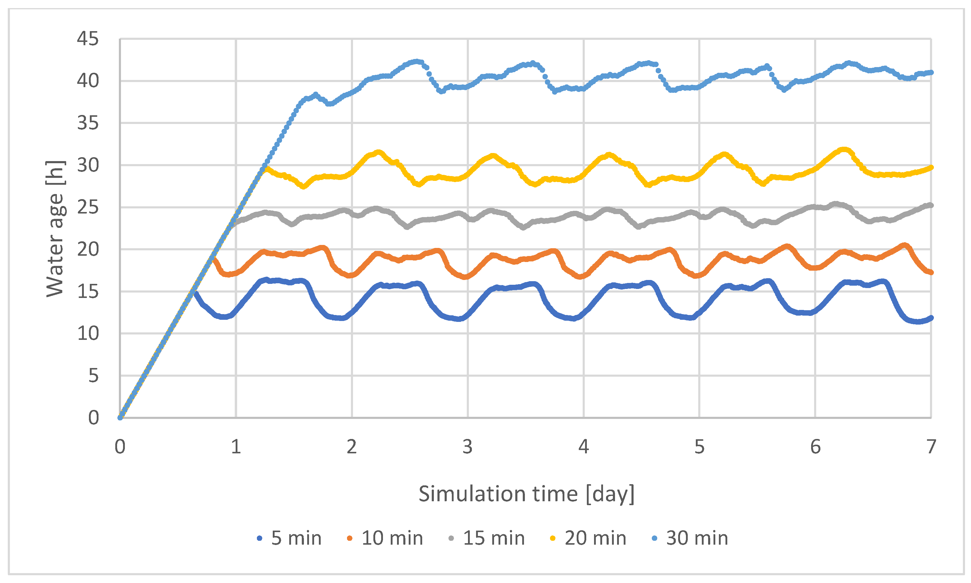
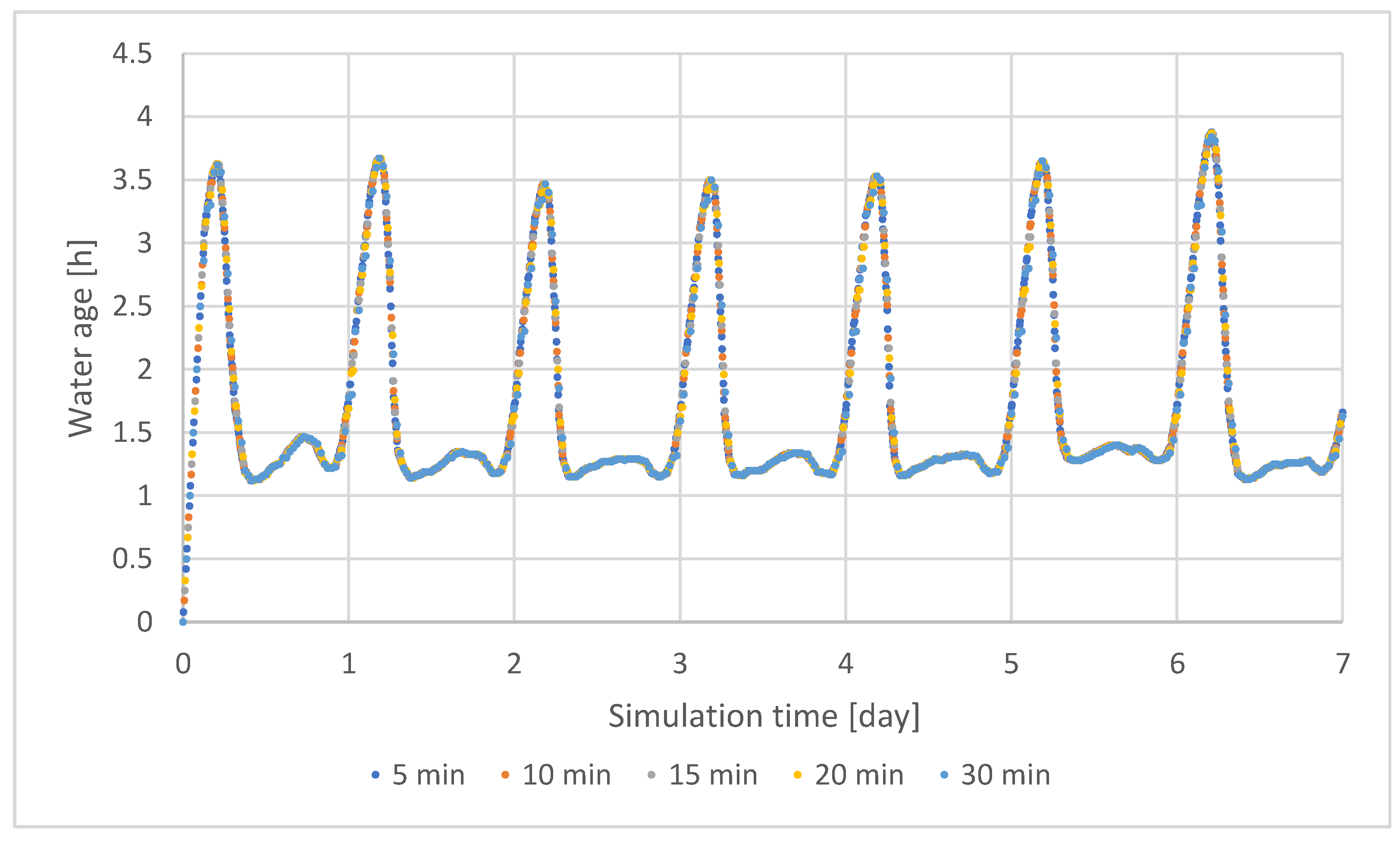
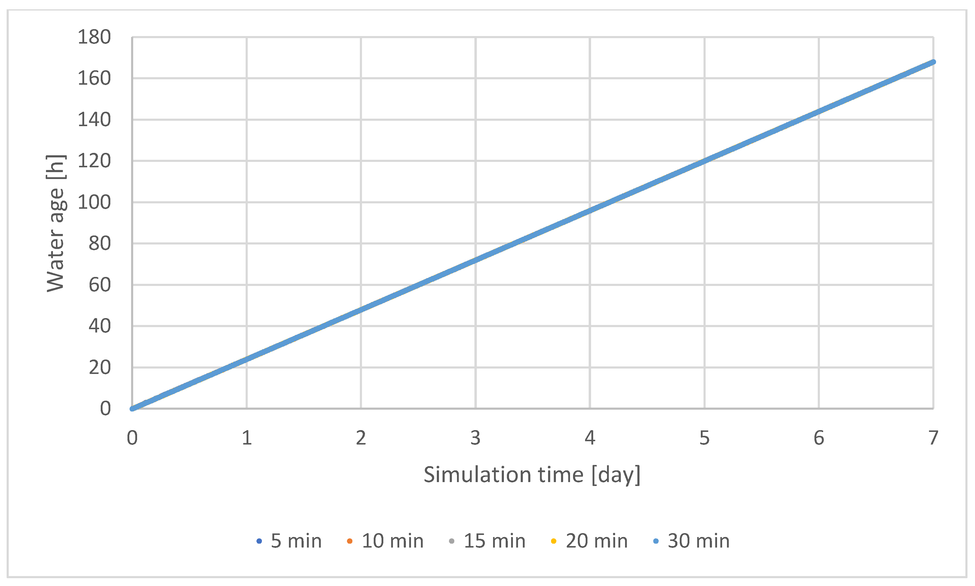
3.3. Influence of Simulation Timestep
3.4. Descriptive Statistics: Influence of Results due to Timestep
4. Discussion
5. Conclusions
Author Contributions
Funding
Institutional Review Board Statement
Informed Consent Statement
Data Availability Statement
Conflicts of Interest
References
- Gwoździej-Mazur, J.; Świętochowski, K. Analysis of the water meter management of the urban-rural water supply system. E3S Web Conf. 2018, 44, 00051. [Google Scholar] [CrossRef]
- Malmur, R.; Mrowiec, M.; Ociepa, E.; Deska, I. Sustainable Water Management in Cities Under Climat Changes. Probl. Ekorozw. 2018, 13, 133–138. [Google Scholar]
- Dzienis, L.; Lebiedowski, M. Water Supply and Water Treatment Systems in Agricultural and Industrial Regions: Selected Problems; HARD: Olsztyn, Poland, 2009. [Google Scholar]
- Denczew, S. Podstawy Modelowania Systemów Eksploatacji Wodociągów I Kanalizacji: Teoria I Praktyka; Polska Akademia Nauk. Komitet Inżynierii Środowiska: Lublin, Poland, 2006. (In Polish) [Google Scholar]
- Gwoździej-Mazur, J.; Świętochowski, K. Evaluation of Real Water Losses and the Failure of Urban-Rural Water Supply System. J. Ecol. Eng. 2021, 22, 132–138. [Google Scholar] [CrossRef]
- Zimoch, I.; Bartkiewicz, E. Modeling of water age as an element supporting the management of the water supply system. Proc. ECOpole 2018, 12, 611–620. [Google Scholar] [CrossRef]
- Wilson, A.I. Hydraulic Engineering and Water Supply. In The Oxford Handbook of Engineering and Technology in the Classical World; Oxford University Press: Oxford, UK, 2009. [Google Scholar] [CrossRef]
- Trębicka, A. A Model of Time Variability of Characteristic Parameters of the Water Distribution System as a Base of Information and the Basis of Mathematical Modelling. J. Ecol. Eng. 2020, 21, 46–51. [Google Scholar] [CrossRef]
- Sitzenfrei, R.; Möderl, M.; Rauch, W. Automatic generation of water distribution systems based on GIS data. Environ. Model. Softw. 2013, 47, 138–147. [Google Scholar] [CrossRef]
- Brenna, L.; Dyrkoren, P.; Vangdal, A.; Poulton, M.; Bruaset, S. Report on System Development, Method Applicability, and Pipeline Condition Data for Modelling Purposes. 2014. Available online: http://hdl.handle.net/10251/35740 (accessed on 2 February 2022).
- National Research Council. Drinking Water Distribution Systems: Assessing and Reducing Risks; National Academies Press: Washington, DC, USA, 2007; Available online: https://nap.nationalacademies.org/catalog/11728/drinking-water-distribution-systems-assessing-and-reducing-risks (accessed on 8 March 2022).
- Kulbik, M. Komputerowa Symulacja i Badania Terenowe Miejskich Systemów Wodociągowych; Monografie 49; Politechnika Gdańska: Gdańsk, Poland, 2004. (In Polish) [Google Scholar]
- Trębicka, A. Efficiency End Optimum Decisions in the Modeling Process of Water Distribution. J. Ecol. Eng. 2018, 19, 254–258. [Google Scholar] [CrossRef]
- Gwoździej-Mazur, J.; Andraka, D.; Kaźmierczak, B.; Kruszyński, W. On-Line Water Consumption Monitoring as a Tool for Optimal Management of Water Distribution Network. Environ. Sci. Proc. 2021, 9, 26. [Google Scholar] [CrossRef]
- Haestad, M.; Walski, T.; Chase, D.V.; Savic, D. Advanced Water Distribution Modeling and Management; Bentley Institute Press: Waterbury, CT, USA, 2004. [Google Scholar]
- Gwoździej-Mazur, J.; Świętochowski, K. Non-Uniformity of Water Demands in a Rural Water Supply System. J. Ecol. Eng. 2019, 20, 245–251. [Google Scholar] [CrossRef]
- Boulos, P.F. Comprehensive Water Distribution Systems Analysis Handbook for Engineers and Planners; American Water Works Association: Washington, DC, USA, 2004. [Google Scholar]
- Studzinski, J. ICS System Supporting the Water Networks Management by Means of Mathematical Modelling and Optimization Algorithms. J. Autom. Mob. Robot. Intell. Syst. 2015, 9, 48–54. [Google Scholar] [CrossRef]
- Clarke, R. Modeling Water Quality in Distribution Systems, 2nd ed.; American Water Works Association Washington DC, USA: 2011. Available online: https://ebookcentral-proquest-com.bazy.pb.edu.pl/lib/bialostocka/reader.action?docID=3116755 (accessed on 10 February 2022).
- Denczew, S.; Królikowski, A. Podstawy Nowoczesnej Eksploatacji Układów Wodociągowych i Kanalizacyjnych; Arkady: Warsaw, Poland, 2002. (In Polish) [Google Scholar]
- Wu, Z.Y.; Boulos, P.F.; Orr, C.H.; Ro, J.J. An Efficient Genetic Algorithm Approach to an Intelligent Decision Support System for Water Distribution Networks. In Proceedings of the 4th International HydroInformatics Conference, Iowa Institute of Hydraulic Research, Iowa City, IA, USA, 23–27 July 2000. [Google Scholar]
- Vairavamoorthy, K.; Yan, J.; Galgale, H.M.; Gorantiwar, S.D. IRA-WDS: A GIS-based risk analysis tool for water distribution systems. Environ. Model. Softw. 2007, 22, 951–965. [Google Scholar] [CrossRef]
- Lewis, A. Rossman and others. In EPANET 2.2 User Manual; U.S. Environmental Protection Agency: Washington, DC, USA, 2020. Available online: https://epanet22.readthedocs.io/_/downloads/en/latest/pdf/ (accessed on 1 February 2022).
- Aurenhammer, F.C.D. Voronoi Diagrams—A Survey of a Fundamental Geometric Data Structure. ACM Comput. Surv. 1991, 23, 345–405. [Google Scholar] [CrossRef]
- Okabe, A.; Satoh, T.; Furuta, T.; Suzuki, A.; Okano, K. Generalized net-work Voronoi diagrams: Concepts, computational methods, and applications. Int. J. Geogr. Inf. Sci. 2008, 22, 965–994. [Google Scholar] [CrossRef]
- Kruszyński, W.; Zajkowski, A. Influence of Level of Detail (LOD) in Hydraulic Model Geometry with Demand Allocation by Voronoi Polygon Method on Chosen Parameters. Environ. Sci. Proc. 2021, 9, 35. [Google Scholar] [CrossRef]
- Guth, N.; Klingel, P. Demand Allocation in Water Distribution Network Modelling—A GIS-Based Approach Using Voronoi Diagrams with Constraints. In Application of Geographic Information Systems; IntechOpen Limited: London, UK, 31 October 2012. [Google Scholar] [CrossRef]
- McKenzie, R.; Wegelin, W. Implementation of pressure management in municipal water supply systems. In Proceedings of the EYDAP Conference “Water: The Day After”, Athens, Greece, 6–8 November 2009; Volume 20. Available online: https://www.miya-water.com/fotos/artigos/03_implementation_of_pressure_management_in_municipal_water_supply_systems_3323280065a328bc009ead.pdf (accessed on 5 February 2022).
- Baader, J.; Fallis, P.; Hübschen, K.; Klingel, P.; Knobloch, A.; Laures, C.; Oertlé, E.; Trujillo Alvarez, R.; Ziegler, D. Guidelines for Water Loss Reduction—A Focus on Pressure Management. 2011. Available online: https://www.researchgate.net/publication/318792810_Guidelines_for_water_loss_reduction_-_a_focus_on_pressure_management (accessed on 7 February 2022).
- Abhijith, G.R.; Kadinski, L.; Ostfeld, A. Modeling Bacterial Regrowth and Trihalomethane Formation in Water Distribution Systems. Water 2021, 13, 463. [Google Scholar] [CrossRef]


| Type of Demand | Number of Demand Points | |
|---|---|---|
| Single-family housing | 1066.00 | 1923 |
| Multi-family housing | 249.98 | 58 |
| Industry | 240.04 | 1 |
| Descriptive Statistics | A-Avrg | B-Avrg | A-Med | B-Med | A-Min | B-Min | A-Max | B-Max |
|---|---|---|---|---|---|---|---|---|
| Valid | 1009 | 1009 | 1009 | 1009 | 1009 | 1009 | 1009 | 1009 |
| Mode | 8.940 * | 13.500 * | 8.490 * | 10.420 * | 2.210 | 2.510 | 40.380 | 71.270 |
| Median | 10.530 | 13.580 | 8.750 | 11.800 | 2.270 | 2.570 | 38.890 | 69.570 |
| Mean | 10.722 | 13.277 | 9.524 | 11.889 | 2.913 | 3.202 | 34.834 | 55.914 |
| Std. Deviation | 2.232 | 2.641 | 2.234 | 2.424 | 1.306 | 1.306 | 10.142 | 22.039 |
| Skewness | −1.444 | −2.426 | −0.686 | −1.886 | 1.300 | 1.276 | −2.030 | −1.176 |
| Std. Error of Skewness | 0.077 | 0.077 | 0.077 | 0.077 | 0.077 | 0.077 | 0.077 | 0.077 |
| Minimum | 0.000 | 0.000 | 0.000 | 0.000 | 0.000 | 0.000 | 0.000 | 0.000 |
| Maximum | 14.440 | 16.550 | 13.150 | 15.100 | 6.430 | 6.730 | 42.120 | 72.470 |
| Descriptive Statistics | Average | Median | Minimum | Maximum |
|---|---|---|---|---|
| Valid | 337 | 337 | 337 | 337 |
| Missing | 0 | 0 | 0 | 0 |
| Mode ᵃ | 0.000 | 39.130 | 1.300 | 0.000 |
| Median | 43.482 | 39.965 | 1.310 | 84.000 |
| Mean | 38.092 | 35.475 | 1.712 | 84.000 |
| Std. Deviation | 12.743 | 10.489 | 0.787 | 48.714 |
| Skewness | −1.417 | −2.021 | 1.373 | 4.155 × 10⁻²⁰ |
| Std. Error of Skewness | 0.133 | 0.133 | 0.133 | 0.133 |
| Minimum | 0.000 | 0.000 | 0.000 | 0.000 |
| Maximum | 49.819 | 42.335 | 3.840 | 168.000 |
| Descriptive Statistics | Mode | Median | Mean | Std. Deviation | Skewness | Std. Error of Skewness | Minimum | Maximum | |
|---|---|---|---|---|---|---|---|---|---|
| Average | 5 min | 0.000 | 20.472 | 19.805 | 5.474 | −1.225 | 0.055 | 0.000 | 27.863 |
| 10 min | 0.000 | 24.689 | 23.261 | 6.434 | −1.507 | 0.077 | 0.000 | 31.148 | |
| 15 min | 27.449 | 29.16 | 26.992 | 7.721 | −1.62 | 0.094 | 0.000 | 35.321 | |
| 20 min | 0.000 | 33.831 | 30.79 | 9.263 | −1.602 | 0.109 | 0.000 | 40.061 | |
| 30 min | 0.000 | 43.482 | 38.092 | 12.743 | −1.417 | 0.133 | 0.000 | 49.819 | |
| Median | 5 min | 15.690 | 14.09 | 13.587 | 2.788 | −2.204 | 0.055 | 0.000 | 16.44 |
| 10 min | 19.500 | 18.85 | 17.691 | 3.596 | −3.131 | 0.077 | 0.000 | 20.52 | |
| 15 min | 23.875 | 23.81 | 22.242 | 5.01 | −2.922 | 0.094 | 0.000 | 25.455 | |
| 20 min | 0.000 | 33.831 | 30.79 | 9.263 | −1.602 | 0.109 | 0.000 | 40.061 | |
| 30 min | 0.000 | 43.482 | 38.092 | 12.743 | −1.417 | 0.133 | 0.000 | 49.819 | |
| Min | 5 min | 1.290 | 1.32 | 1.713 | 0.782 | 1.396 | 0.055 | 0.000 | 3.88 |
| 10 min | 1.290 | 1.32 | 1.713 | 0.783 | 1.391 | 0.077 | 0.000 | 3.87 | |
| 15 min | 1.280 | 1.31 | 1.713 | 0.784 | 1.387 | 0.094 | 0.000 | 3.86 | |
| 20 min | 0.000 | 33.831 | 30.79 | 9.263 | −1.602 | 0.109 | 0.000 | 40.061 | |
| 30 min | 0.000 | 43.482 | 38.092 | 12.743 | −1.417 | 0.133 | 0.000 | 49.819 | |
| Max | 5 min | 5.180 | 84 | 84.005 | 48.525 | 4.122 × 10⁻⁴ | 0.055 | 0.000 | 168 |
| 10 min | 0.000 | 84 | 84.001 | 48.567 | 1.156 × 10⁻⁴ | 0.077 | 0.000 | 168 | |
| 15 min | 0.000 | 84 | 84.001 | 48.604 | 9.511 × 10⁻⁵ | 0.094 | 0.000 | 168 | |
| 20 min | 0.000 | 33.831 | 30.79 | 9.263 | −1.602 | 0.109 | 0.000 | 40.061 | |
| 30 min | 0.000 | 43.482 | 38.092 | 12.743 | −1.417 | 0.133 | 0.000 | 49.819 | |
Publisher’s Note: MDPI stays neutral with regard to jurisdictional claims in published maps and institutional affiliations. |
© 2022 by the authors. Licensee MDPI, Basel, Switzerland. This article is an open access article distributed under the terms and conditions of the Creative Commons Attribution (CC BY) license (https://creativecommons.org/licenses/by/4.0/).
Share and Cite
Zajkowski, A.; Kruszyński, W.; Bartkowska, I.; Wysocki, Ł.; Krysztopik, A. Influence of Hydraulic Model Complexity on Results of Water Age and Quality Simulation in Municipal Water Supply Systems. Sustainability 2022, 14, 13701. https://doi.org/10.3390/su142113701
Zajkowski A, Kruszyński W, Bartkowska I, Wysocki Ł, Krysztopik A. Influence of Hydraulic Model Complexity on Results of Water Age and Quality Simulation in Municipal Water Supply Systems. Sustainability. 2022; 14(21):13701. https://doi.org/10.3390/su142113701
Chicago/Turabian StyleZajkowski, Artur, Wojciech Kruszyński, Izabela Bartkowska, Łukasz Wysocki, and Anna Krysztopik. 2022. "Influence of Hydraulic Model Complexity on Results of Water Age and Quality Simulation in Municipal Water Supply Systems" Sustainability 14, no. 21: 13701. https://doi.org/10.3390/su142113701
APA StyleZajkowski, A., Kruszyński, W., Bartkowska, I., Wysocki, Ł., & Krysztopik, A. (2022). Influence of Hydraulic Model Complexity on Results of Water Age and Quality Simulation in Municipal Water Supply Systems. Sustainability, 14(21), 13701. https://doi.org/10.3390/su142113701