Does Innovative Industrial Agglomeration Promote Environmentally-Friendly Development? Evidence from Chinese Prefecture-Level Cities

Abstract

China has promised to meet the “carbon peaking and carbon neutrality” goals. Exploring the relationship between innovative industrial agglomeration and environmental pollution plays an important role in the realization of these goals and sustainable development. Based on the panel data of 277 prefecture-level cities in China from 2007 to 2019, this paper uses the multi-period difference-in-difference (DID) model to examine the impact and mechanism of the innovative industrial agglomeration pilot (IIAP) policy on the environment. Furthermore, we explore the spatial effect of the IIAP using spatial DID. The findings show that, firstly, the IIAP policy significantly contributes to environmentally-friendly development in terms of enhancing carbon emission efficiency (CEE) and reducing environmental pollution index (EPI). Secondly, the IIAP policy promotes environmentally-friendly development mainly by improving the technological innovation level. Additionally, the heterogeneity analysis shows that the environmentally-friendly effect of the IIAP policy is primarily in the eastern region, large cities, and non-resource-based cities. Finally, there is a significant spatial effect of the IIAP policy on environmentally-friendly development, mainly reflected in the weak siphon effect between treatment group cities and neighboring regions. We suggest that the government should continue to maintain the steady growth of the IIAP cities and improve the energy utilization efficiency through a policy of green technology innovation. The government should also optimize the spatial layout of the pilot cities and make full use of the energy advantages of each region to better promote environmentally-friendly development.

1. Introduction

The advancement of informatization, the rapid growth of biotechnology, and the Internet are changing the economic production pattern and market structure [1]. Scientific and technological innovation is spreading to all fields of society and gradually becoming the main driving force of global economic development. In recent years, the United States, Germany, Japan, Russia, and other countries have launched national innovation strategies, which regard innovation ability as the core of comprehensive national strength competition [2]. Similarly, in China, innovation-driven development has become the new trend in economic development [3]. Accelerating the cultivation of innovative industries has already been a strategy for China’s economic development [4]. 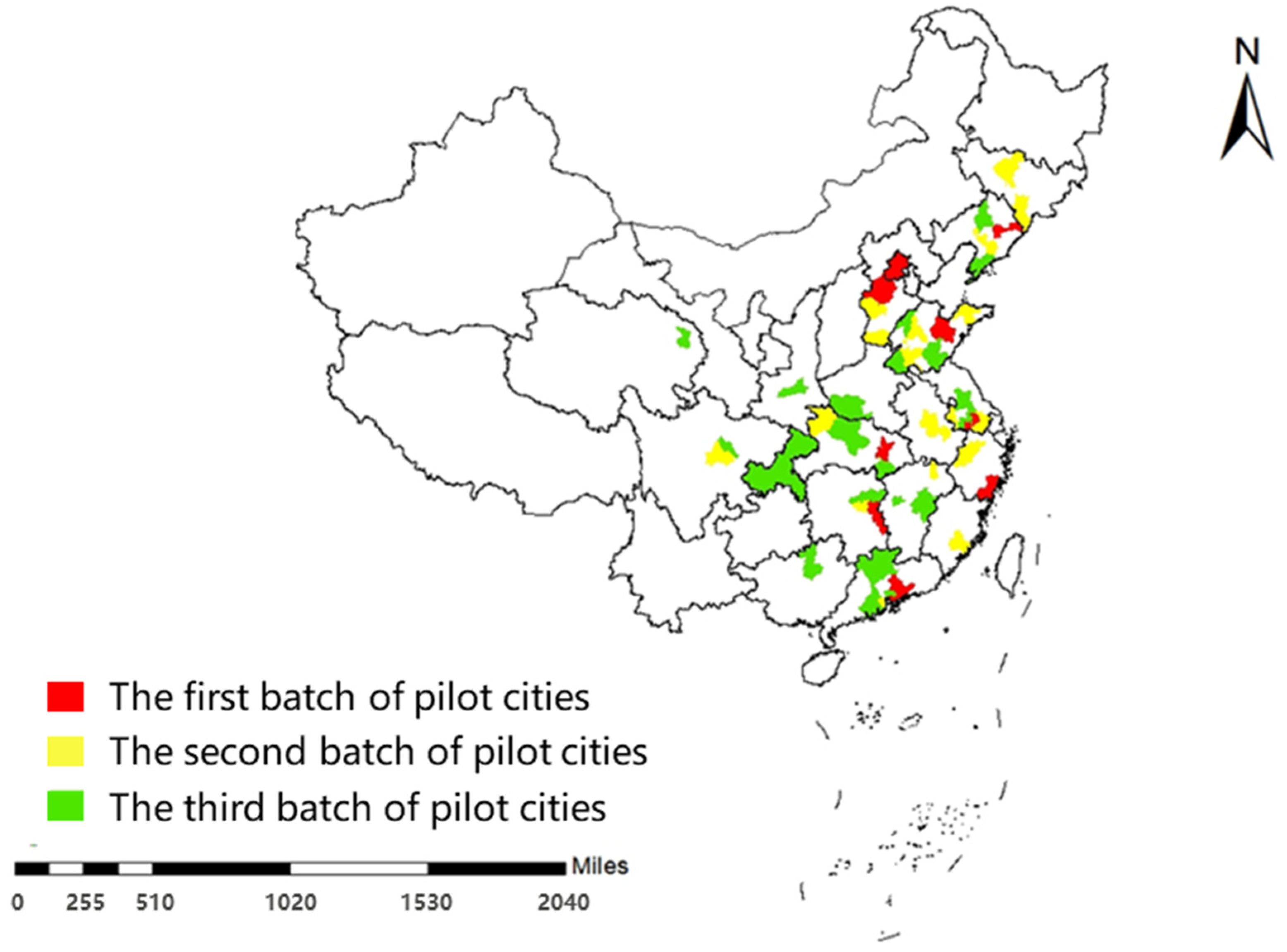Based on the traditional industrial agglomeration, innovation industrial agglomeration emphasizes agglomeration development with innovation as the core [5]. It refers to the gathering of enterprises, R&D, and service institutions related to the industrial chain in a specific region to form a cross-industry and cross-regional industrial organization form through a division of labor and cooperation, and collaborative innovation. The IIAP is focused on high-tech and strategic new industries. Since the Ministry of Science and Technology of China officially started to implement the first batch of innovative industrial agglomeration pilots (IIAP) in 2013, China attached importance to its development and then gradually expanded the pilot scope in 2014 and 2017. By 2020, China had gradually laid out 48 innovative industrial agglomeration pilot construction units and 61 innovative industrial agglomeration pilot units, involving 55 prefecture-level cities.

Unlike traditional industrial agglomeration, innovative industrial agglomeration gathers more innovative enterprises in a particular geographical area. The phenomenon of agglomeration can push the integration of industrial resources, optimize the upgrading of industrial structure and, thus, promote economic growth [6]. At the same time, the agglomeration development will use a large number of internal and external resources in the agglomeration area, leading to excessive centralization of population, which will also bring different levels of influence to the surrounding environment [7]. China is a major carbon emitter and is under greater pressure to save energy and reduce emissions in economic development [8]. Therefore, it has become an essential requirement for China’s development to implement green transformation, to undertake green and low-carbon energy development, and to adhere to the development path of ecological priority [9]. As a vital combination of China’s innovation strategy and industrial agglomeration development, the IIAP plays a vital role in enhancing industrial innovation capability and regional economic development. However, it remains to be further verified whether the IIAP will bring different impacts on the internal and external environment of the cluster region while promoting industrial economic development.

Industrial agglomeration is a form of spatial organization based on the depth of labor division. It is essential for the optimization of resource allocation and stimulating enterprise innovation through knowledge spillover and incremental returns to scale [10]. Moreover, theoretical studies related to new geography economics suggested that technology externalities and knowledge spillovers are the main impetus for enterprise innovation in agglomeration regions [11]. At the same time, technological advancement and increased innovation levels play a crucial role in pollution control [12]. The industry provides a collaborative innovation environment for enterprises in the agglomeration area through technology spillover, which enhances the efficiency of clean technology R&D and promotes pollution reduction [13]. Therefore, industrial agglomeration and emission reduction may be intrinsically linked. Furthermore, the impact of industrial agglomeration on the environment has received interest from scholars. Quite a few studies have revealed that industrial agglomeration significantly promotes carbon emissions [14]. In contrast, some scholars also believe that industrial agglomeration inhibits carbon emissions [15]. Similarly, a few studies show a nonlinear relationship with carbon emissions [16]. First, the IIAP is to enhance the innovation development of high technology enterprises through policy incentives. Under the stimulus of the policy, the local government will play a leading function and bring in more resource elements, thus, providing a good environment for the implementation of the IIAP. Second, the sources of pollution emissions should be measured comprehensively. Under the government’s guidance, industrial agglomeration can increase energy utilization [17]. Labor concentration can also cause excessive consumption of raw materials and wastewater discharge [18]. Therefore, the impact of agglomeration on the environment cannot be achieved simply by carbon emissions, but also by considering major environmental pollutants, such as sulfur dioxide, soot, wastewater, PM2.5, etc. In addition, the impact of the IIAP on the environment may have a spatial effect. Since the implementation of the IIAP, the number of pilot units has been increasing, and the area involved has been gradually expanded. The natural resources of neighboring cities are similar [19]. The technology and innovation brought to the local area by the IIPA can be copied and learned from by neighboring cities. They may also have some impact on the surrounding environment. Therefore, whatever the effect of the IIAP on the environment, it can be studied by neighboring regions, which can contribute to the promotion of ecological efficiency levels and contribute to environmentally-friendly development.

This paper explores the impact of the innovative industrial agglomeration pilot (IIAP) policy on the environment and conducts in-depth analysis of carbon efficiency and the environmental pollution index. Specific contributions are as follows: first, from the existing research, work on pilot policies and the environment have made remarkable achievements in other pilot policies, such as the low-carbon pilot and innovative city pilot. However, there have been relatively few studies on the innovative industrial agglomeration pilot policy. Hence, this paper selects the IIAP to further examine the impact of the IIAP policy on the environment. Second, when existing studies measure the impact of the pilot policy on the environment, most of them only analyze from the perspective of carbon emissions. In contrast, this paper comprehensively examines the impact of the IIAP on the environment. We construct an environmental pollution index using the primary environmental pollutants sulfur dioxide, wastewater, soot, and PM2.5, and examine the carbon emissions efficiency and the environmental pollution index. Finally, our study constructs a spatial DID model to further investigate the spatial effects of the IIAP.

The structure of this paper is as follows. Section 2 reviews the literature on the IIAP and environmentally-friendly development and puts forward the research hypothesis of this paper. Section 3 introduces the data sources and variable definitions, and then establishes the multi-period difference-in-difference (DID) model and mediating effect model. Section 4 reports the empirical results and data analysis. Section 5 explores spatial spillover effect of the IIAP using spatial DID. Section 6 draws conclusions, makes relevant policy recommendations, and presents the shortcomings and outlook of this paper.

2. Literature Review

2.1. The Impact of the IIAP on Environment

There are controversies among different scholars about the effects of industrial agglomeration on the environment. The existing studies on the relationship between the two are divided into three main views. The first is that industry agglomeration promotes environmentally-friendly development [20]. Zhang, Rong, Qin, and Ji [21] investigated the impact of industrial clusters and carbon dioxide in 18 cities in Henan Province through the space panel model, and found that the agglomeration phenomenon can optimize the industrial structure, reducing carbon emissions. Using the data of 259 prefecture-level cities in China, Chen, Sun, and Lan [22] examined the impact of industrial agglomeration on the environment from multiple perspectives, including wastewater, sulfur dioxide, soot, and ecological efficiency, and concluded that industrial agglomeration could reduce environmental pollution and effectively improve ecological efficiency through a spatial Durbin model. The second view is that industrial agglomeration accelerates environmental pollution [23]. Han, Xie, Lu, Fang, and Liu [24] used the data of 283 prefecture-level cities in China from 2003–2010 to investigate the impact of urban agglomeration on carbon emissions using a spatial econometric model, and found that the centralization of industries in a specific spatial and geographical area increases energy consumption, resulting in a significant increase in carbon emissions. Yuan, Feng, Lee, and Cen [25] pointed out that environmental externalities became increasingly visible, and pollution problems would become increasingly severe after a certain industrial agglomeration level. The third view is that there is a nonlinear relationship between industrial agglomeration and environmental pollution [26]. Huang, Wang, Cheng, and Dai [27] found that the agglomeration effect of tourism enterprises in developed regions had a U-shaped relationship with the carbon emission of local and neighboring regions through spatial econometric models, and for less developed regions the agglomeration effect has an inverted U-shaped relationship. On the one hand, introducing the pilot policy will increase government subsidies to innovative enterprises and improve R&D efficiency and resource utilization. On the other hand, the pollution caused by the agglomeration process can be treated centrally, reducing the cost of pollution control. Therefore, the introduction of the IIAP may promote environmentally-friendly development. Based on the above analysis, the following hypotheses are proposed:

H1. 

The IIAP has a significantly positive effect on carbon efficiency;

H2. 

The IIAP significantly reduces environmental population.

2.2. The Mechanism Analysis of the IIAP

Innovative industrial agglomeration promotes the upgrading of industrial structure, breaks through the low-end lock of traditional industrial clusters, and contributes to improvements in technological innovation. In the meantime, the promotion of the pilot policy has improved the resource utilization rate of industries in the agglomeration area, laying an excellent environmental foundation for the implementation of the pilot [28].

Firstly, most scholars believed that the promotion of pilot policy and the implementation of industrial agglomeration could increase the motivation of enterprises’ R&D and promote technological innovation. Hu, Li, and Tang [29] assessed the pilot policy of carbon trading in Beijing, China, and found that technological innovation should be strengthened to achieve better emission reduction. Cheng, Yi, Dai, and Xiong [30] examined the relationship between low-carbon pilot policy and green growth through the difference-in-difference (DID) model and found that the spread of the low-carbon pilot policy was beneficial to the level of urban innovation through the difference-in-difference (DID) model. Li, Lai, and Zhang [31] examined the effect of agglomeration level on green innovation under the effect of environmental regulation by constructing a moderating effect model, and found that when environmental regulation promotes agglomeration innovation, diversified enterprise agglomeration was conducive to enhancing enterprise green technology innovation. Zhang and Wang [32] used the threshold to examine impact of industry clusters on innovation efficiency, and the study found that industrial agglomeration can promote innovation efficiency before reaching the threshold.

Secondly, pilot policy and industry agglomeration can also influence the environment through technological innovation. The implementation of the pilot policy will stimulate innovation and effectively improve the R&D efficiency and energy utilization rate of enterprises [33] and, therefore, can promote environmentally-friendly development. Huo, Qi, Wang, Liu, and Zhou [34] found that pilot cities could achieve emission reduction through enterprise technology innovation to improve total factor productivity and promote research and development of low-carbon technology. Yu, Chen, and Zhang [35] used the multi-period difference-in-difference (DID) model to study the impact of innovative pilot policy on energy productivity in China and revealed that the pilot policy reduced energy costs through technological innovation, accelerated energy transition and, thus, increased urban energy productivity. Liu and Zhang [36], based on the industrial departments of 30 provinces in China from 1998 to 2017, used the spatial Durbin model to investigate the relationship between industrial agglomeration, technological innovation, and carbon emission efficiency, and found that there is an inverted U-shaped relationship between industrial clusters and carbon efficiency, and that technological innovation plays an important role in them. In summary, the impact of innovative industrial agglomeration pilot policy on the environment is currently less discussed. Most studies argued that the promotion of pilot policy and the implementation of industrial agglomeration can improve the technological innovation of enterprises. It further improves the efficiency of resource utilization and has a certain impact on the environment. This leads to the following hypotheses:

H3. 

Technological innovation has a mediating role between the IIAP and carbon efficiency;

H4. 

Technological innovation has a mediating role between the IIAP and environment population.

3. Study Design

3.1. Data

This paper selects the data of 277 prefecture-level cities in China from 2007 to 2019 as the research sample. This excludes the samples that were withdrawn or established in prefecture-level cities during the sample period (such as Chaohu City and Sansha City, etc.) and the samples with serious data missing. The data are mainly from the China Urban Statistical Yearbook and the China Statistical Yearbook over the years. The PM2.5-related data come from the Atmospheric Composition Analysis Group of Dalhousie University in Canada. Technological innovation index data come from the Chinese Research Data Services Platform (CNRDS). Carbon dioxide emissions data from 2006 to 2019 are from the China Emission Accounts and Datasets (CEADs) [37]. Relevant IIAP data was obtained from the Ministry of Science and Technology of China. After excluding the missing observations, 55 pilot cities remain in the sample (a distribution map is shown in the Appendix A, Figure A1).

3.2. Variables

3.2.1. Dependent Variables

Carbon emission efficiency (CEE) is a dependent variable. This paper measures the CEE of 277 prefecture-level cities in China using the Super-SBM model. We suppose that there are n decision-making units (DMUs). Each DMU has the m input, r₁ desirable output, and r₂ undesirable output, respectively (see

Table A1. Inputs and outputs for calculating CEE.

Type	Variables	Detail
Input	Employment population	Measured by the total employed population at the end of the year.
	Capital stock	Ki,t = Ki,t−1(1 − δi,t) + Ii,t, Ki,t, Ii,t, δi,t represent capital stock, total fixed asset formation and economic depreciation rate, respectively. Following Zhang, Rong, Qi and Ji [1], the economic depreciation rate is 9.6%.
	Energy consumption	Ei,t = K1 × Mi,t + K2 × Ni,t + K3 × Pi,t. Here, Ei,t is the converted total amount of standard coal; Mi,t, Ni,t, Pi,t are the consumption of natural gas, liquefied petroleum gas and electricity respectively; K1, K2, K3 are the conversion coefficients.
Output	Desirable output: real GDP	Taking the base period of 2006, the GDP deflator is carried out, and the deflator index is replaced by the provincial index.
	Undesirable output: carbon emissions	The data comes from the research of Shan, Guan, Hang, Zheng, Li, Guan, Li, Zhou, Li, and Hubacek [54] in the CEADs database.

in Appendix A for detailed data). Then, the matrix of input, desirable output, and undesirable output can be defined as follows: $X=\left[x_1,x_2\cdots x_n\right]\in R^{m\times n}$, $Y=\left[y_1,y_2\cdots y_n\right]\in R^{r_1\times n}$, $Z=\left[z_1,z_2\cdots z_n\right]\in R^{r_2\times n}$.

Referring to Pastor and Lovell [38], a Super-SBM model under the condition of constant returns to scale (CRS) is constructed, and the formula is as follows:

$$\begin{gathered} \rho =\min \frac{1+\frac{1}{m}{{\displaystyle \sum }}_{i=1}^m\frac{s_i^{-}}{x_{iq}}}{1-\frac{1}{r_{1+}{r}_2}\left({{\displaystyle \sum }}_{k=1}^{r_1}\frac{s_k^{+}}{x_{kq}}+{{\displaystyle \sum }}_{l=1}^{r_2}\frac{s_l^{-}}{x_{lq}}\right)} \\ s.t.\{\begin{array}{c}{x}_{iq}⩾{\displaystyle \sum }_{j=1,j\ne q}^n{x}_{ij}{\lambda }_j-s_i^{-}\\ y_{kq}⩽{\displaystyle \sum }_{j=1,j\ne q}^n{y}_{kj}{\lambda }_j+s_k^{+}\\ z_{lq}⩾{\displaystyle \sum }_{j=1,j\ne q}^n{z}_{lj}{\lambda }_j-s_l^{-}\\ {\lambda }_j,s_i^{-},s_k^{+},s_l^{-}⩾0,\forall i,k,l,j,q,q\ne j\end{array} \end{gathered}$$

(1)

where ρ represents the efficiency value of the DMU, x_iq, y_kq, z_lq represent input, desirable output, and undesirable output, respectively, and s_i⁻, s_k⁺, s_l⁻ are slack variables for three factors. Finally, λ_j is the weight of input and output of the t DMU.

The global Malmquist–Luenberger index (GML) was proposed by Pastor and Lovell [38]. Compared with the traditional Malmquist–Luenberger index (ML), the GML can effectively avoid the problem of unsolvable linear programming. The GML can also reflect economic production activities more realistically [39]. Therefore, the GML index can more accurately reflect the dynamic change in carbon emission efficiency. The GML is calculated as follows:

$$GM{L}_t^{t+1}\left(x^{t+1},y^{t+1},z^{t+1},x^t,y^t,z^t\right)=\frac{E_c^g\left(x^{t+1},y^{t+1},z^{t+1}\right)}{E_c^g\left(x^t,y^t,z^t\right)}$$

(2)

where $GM{L}_t^{t+1}$ is the ratio of productivity in t + 1 to t and reflects the growth rate of CEE from t to t + 1. Here, $GM{L}_t^{t+1}$ > 1 means that the CEE is improved, while $GM{L}_t^{t+1}$ < 1 means that the CEE is decreased. When $GM{L}_t^{t+1}$ = 1, it means that the CEE is unchanged. Therefore, we choose 2006 as the base period, and the CEE in 2007 is the GML from 2006 to 2007. By analogy, we calculate the CEE of all 277 prefecture-level cities in China from 2007 to 2019.

The environmental pollution index (EPI) is another dependent variable. To comprehensively analyze the impact of the IIAP on the environment, this paper constructs a new environmental measurement index based on the research of Dong, Wang, Zheng, Li, and Xie [25]. The new index EPI is calculated by the principal component analysis method (PCA), including four sub-indicators of industrial smoke and dust emissions, wastewater discharges, sulfur dioxide emissions, and PM2.5.

3.2.2. Explanatory Variable

The implementation of the IIAP policy (DID) is the explanatory variable. In this paper, the cities that belong to the IIAP are taken as the treatment group, with other cities as the control group. At the same time, we construct two dummy variables. The first is the city dummy variable (treat). If the city is the pilot city, treat takes the value 1; otherwise, it is 0. (2) The second is the policy time dummy variable (post). The post value of the pilot city in the treatment group is 1 in the year and after the establishment, and the value of post in the control group city is always 0. The DID is the interactive item between treat and post, that is, DID_i,t = treat_i × post_t, which means that if city i was set up as a pilot city in year t, then DID equals 1; otherwise, it equals to 0.

3.2.3. Mediation Variable

Technological innovation (Inn) is the mediation variable. The existing measurement indicators of technological innovation mainly involve regional innovation output, the number of patent applications and patent grants, etc. [40]. We consider that the research topic of this paper involves environmental protection and the lagging effect of policy implementation. Therefore, we choose the sum of the number of general patents (invention patents, utility patents, and design patents) and green innovation patents obtained by the city in the current year to measure technological innovation. To reduce the impact of data difference, the natural logarithm is taken.

3.2.4. Control Variables

This paper refers to Zhu, Zhang, Huang, Wang, and Su [41] to control the following variables: (1) economic development (Eco) is measured by the logarithmic value of the GDP of each prefecture-level city; (2) labor endowment (Labor) is the proportion of employees to the total population at the end of the year; (3) openness (Open) is measured by the percentage of actual foreign investment in GDP; (4) financial size (Fin) is measured using the logarithm of the number of employees in the financial industry; (5) industrial upgrading level (Ind) is expressed as the ratio of primary industry value added to GDP × 1 + the ratio of secondary industry value added to GDP × 2 + the ratio of tertiary industry value added to GDP × 3; (6) Urbanization (Urb) is the ratio of urban construction land to total area; (7) scientific and technological development (RD) is measured using the logarithm of the scientific; (8) Internet level (Int) is expressed by the logarithm of the number of Internet users. The descriptive statistics are shown in

Table 1. Descriptive statistical results.

Variable	N	Mean	S.D.	Min	Max	Skewness	Kurtosis	Jarque-Bera Test
CEE	3601	1.0335	0.1239	0.3473	2.1987	0.6696	12.0150	1.25 × 104	0.0000
EPI	3601	−1.08 × 10−9	0.6282	−1.0953	10.3199	2.8754	31.5916	1.28 × 105	0.0000
Eco	3601	16.3600	0.9854	13.3348	19.7609	0.3177	3.1660	64.7019	0.0000
Labor	3601	0.1249	0.1184	0.0238	1.4731	4.6462	35.7194	1.74 × 105	0.0000
Open	3601	0.0183	0.0188	1.77 × 10−6	0.1988	2.0649	10.7480	1.16 × 104	0.0000
Fin	3601	9.3832	0.8796	6.3969	13.3767	0.5874	4.1973	422.1581	0.0000
Ind	3601	2.2674	0.1437	1.8309	2.8322	0.4473	3.3475	3.04 × 104	0.0000
Urb	3601	0.0871	0.0967	0.0002	0.9718	2.8500	16.0339	219.9798	0.0000
RD	3601	10.0405	1.4483	6.1506	15.5293	0.5666	3.4267	49.5559	0.0000
Int	3601	13.0262	1.1042	5.4681	17.7617	−0.0410	3.5688	138.2294	0.0000
Inn	3601	5.7802	1.5981	0.2624	10.7777	0.2094	3.0412	26.5809	0.0000

.

3.3. Model Settings

3.3.1. Benchmark Model

By the end of 2019, three batches of pilot cities for innovative industrial agglomeration have been established. To accurately measure the environmental effects of this policy, this paper refers to the practice of Beck, Levine, and Levkov [42], and constructs the following multi-period DID model:

$$Y_{i,t}={\alpha }_0+{\alpha }_{1}DI{D}_{i,t}+\alpha {\displaystyle \sum }{X}_{i,t}+{\mu }_i+{\gamma }_t+{\epsilon }_{i,t}$$

(3)

where i represents the prefecture-level city, t represents the year, and Y_i,t is the dependent variable representing CEE_i,t and EPI_i,t. The core explanatory variable DID_i,t indicates whether city i implements the innovative industrial agglomeration pilot policy in year t. If city i is set up as a pilot city, the DID value is 1 in the current year and later; otherwise, the DID value is 0. Here, X_i,t represents control variables, including Eco, Labor, Open, Fin, Ind, Urb, Rd, Int, while μ_i is the individual fixed effect, and γ_t is the time fixed effect. Finally, ε_i,t is the random perturbation terms.

3.3.2. Mediation Effect Model

The impact of the IIAP policy on the environment may be realized by upgrading the level of technological innovation. Therefore, referring to Baron and Kenny [43], a mediation effect model was conducted to test the mechanism of the IIAP policy on the environment. Based on Formula (3), the remaining models are as follows:

$$In{n}_{i,t}={\lambda }_0+{\lambda }_{1}DI{D}_{i,t}+\lambda {\displaystyle \sum }{X}_{i,t}+{\mu }_i+{\gamma }_t+{\epsilon }_{i,t}$$

(4)

$$Y_{i,t}={\rho }_0+{\rho }_{1}DI{D}_{i,t}+{\rho }_{2}In{n}_{i,t}+\rho {\displaystyle \sum }{X}_{i,t}+{\mu }_i+{\gamma }_t+{\epsilon }_{i,t}$$

(5)

where Inn_i,t is the mediation variable representing technological innovation, X_i,t is the control variable, and the definition of the variable is the same as above.

4. Empirical Results

4.1. Unit Root Test

In order to prevent the problem of “pseudo-regression”, a unit root test is conducted before the regression analysis to ensure the stability of the time series. The test results are shown in

Table 2. Unit root test.

Variables	HT Test			IPS Test
	Statistic	z	p-Value	Statistic	p-Value
CEE	−0.1731	−37.8350	0.0000	−3.1866	0.0007
EPI	−0.0149	−28.9454	0.0000	−9.8018	0.0000
Eco	0.6580	8.8793	1.0000	−3.4936	0.0002
Labor	0.3881	−6.2971	0.0000	−2.9314	0.0017
Open	0.2193	−16.0832	0.0000	−2.5657	0.0051
Fin	0.2730	−12.7629	0.0000	−28.6918	0.0000
Ind	0.7562	−2.2427	0.0125	−16.1366	0.0000
Urb	0.2689	−12.9915	0.0000	−14.8832	0.0000
RD	0.3339	−9.3357	0.0000	3.1903	0.9993
Int	0.0493	−25.3343	0.0000	−2.8428	0.0022
Inn	0.4486	−2.8879	0.0019	3.1140	0.9991

. In the tests of CEE, EPI, Labor, Open, Fin, Ind, Urb, and Int, the p values are all less than 0.05, indicating that the original hypothesis is rejected, that is, there is no unit root and the series is stable. At least one of the test results of other variables shows that there is no unit root, which can be used for effective panel regression analysis.

4.2. Parallel Trend Test

Referring to the practice of Jacobson and Sullivan [44], we use the event analysis method to test the parallel trend and observe whether there is a time-lag effect in the policy. The specific model is constructed as follows:

$$Y_{i,t}={\beta }_0+{\displaystyle \sum }_{k⩾-4}^6{\beta }_k{D}_k+\beta {\displaystyle \sum }{X}_{i,t}+{\lambda }_i+{\gamma }_t+{\epsilon }_{i,t}$$

(6)

where D₀ is the dummy variable of the year when the pilot policy is implemented, K < 0 means k years before the policy implementation, and k > 0 means k years after the policy implementation. This paper takes 2013 as the benchmark period for policy implementation and sets the detection range as −4 < k < 6. It can be seen from

Table 3. Parallel trend test (CEE).

Variables	CEE	Coefficient
D−4	−0.0286 *	(0.0165)
D−3	0.0175	(0.0149)
D−2	0.0096	(0.0126)
D−1	0.0041	(0.0174)
D0	0.0421 **	(0.0190)
D1	0.0391 *	(0.0154)
D2	0.0123	(0.0183)
D3	0.0829 ***	(0.0298)
D4	0.0151	(0.0241)
D5	−0.0072	(0.0240)
D6	0.0251	(0.0339)
Controls	Y
City FE	Y
Year FE	Y
N	3601
R2	0.2030

Note: *, **, and *** indicate statistical significance at the levels of 10%, 5%, and 1%, respectively.

that the coefficient β_k is basically insignificant before the implementation of the policy. This shows that the CEE changes in the same trend before the implementation of the IIAP policy, which satisfies the parallel trend assumption. Figure 1 shows that the impact of the IIAP on EPI also meets the requirements of the parallel trend. That is, the effect of suppressing environmental pollution is sustainable.

4.3. Benchmark Regression Results

Table 4. Benchmark regression results.

Variables	(1)	(2)	(3)	(4)
	CEE	CEE	EPI	EPI
DID	0.0205 **	0.0261 ***	−0.1264 ***	−0.1114 ***
	(0.0086)	(0.0096)	(0.0380)	(0.0364)
Eco		0.2336 ***		0.0426
		(0.0247)		(0.0589)
Labor		−0.2746 ***		−0.4047 ***
		(0.1043)		(0.1064)
Open		0.1593		−0.5421
		(0.1852)		(0.3960)
Fin		−0.0225 **		0.0035
		(0.0110)		(0.0277)
Ind		0.0940		−0.4651 **
		(0.0775)		(0.1804)
Urb		0.0722		0.0943
		(0.0459)		(0.1461)
RD		−0.0088		−0.0486 ***
		(0.0058)		(0.0134)
Int		−0.0196 ***		0.0136
		(0.0069)		(0.0152)
Cons	1.0706 ***	−2.2438 ***	0.1711 ***	0.8166
	(0.0063)	(0.4433)	(0.0124)	(0.9620)
City FE	Y	Y	Y	Y
Year FE	Y	Y	Y	Y
N	3601	3601	3601	3601
R2	0.1388	0.1990	0.4008	0.4071

Note: ** and *** indicate statistical significance at the levels of 5%, and 1%, respectively.

reports the benchmark regression results of CEE and EPI. The models all controlled for city and year fixed effects simultaneously. Columns (1) and (3) show the regression results without control variables, the columns (2) and (4) are the regression results including control variables. All results show that the coefficient of DID is significant, which indicates that innovative industrial agglomeration can significantly promote environmentally-friendly development. Specifically, the regression results in column (2) show that the coefficient DID is significantly positive at the level of 5%, indicating that the establishment of the IIAP significantly reduces the carbon emissions. Therefore, hypothesis H1 is initially verified. From the results in column (4), the coefficient DID is significantly negative at the level of 1% (α =−0.1114 < 0, p < 0.01), indicating that the IIAP policy can effectively reduce the EPI, improving the environmental, that is, hypothesis H2 is verified.

As can be seen from the control variable results, we take the industrial upgrading level (Ind) of column (2) and column (4) as an example. The Ind is not significant for CEE at the 10% level, but the coefficient is positive. It indicates that the higher the industrial upgrading level, the higher the CEE, to a certain extent. Similarly, the industrial upgrading level has a significant negative impact on the EPI at the level of 5%, indicating that the industrial upgrading level has a positive impact on reducing environmental pollution.

4.4. Robustness Test

4.4.1. Placebo Test

Although a large number of urban characteristic variables have been controlled in quasi-nature experiments, there may still be some non-observed urban characteristic factors that affect the evaluation effect of IIAP. We refer to the method of Yang, Lin, and Li [45] and Sun and Li [46], and use counterfactual methods to conduct the placebo test by randomly generating the pseudo-treatment group dummy variable treat^random and pseudo-policy impact dummy variable post^random. Specifically, we conduct 500 random samplings on the sample data and a repeated regression based on the benchmark model (3). We randomly select 55 cities each time as the treat group, and the policy time is given randomly, and finally obtain 500 groups of interaction terms DID^random (i.e., treat^random × post^random). If the regression coefficient of the DID^random is not significant, it indicates that the environmentally-friendly effect is due to the IIAP, rather than other unobservable factors. Otherwise, the estimation results are not robust. Furthermore, the kernel densities of the 500 estimated coefficients and their p values for each of the two data sets are presented separately in Figure 2. The results show that the randomly generated estimated coefficients are mainly concentrated around 0 and that most of the p values are greater than 0. The actual estimated coefficients of the policy (the vertical dotted lines represent the true coefficients 0.0261 and −0.1114, separately) are significantly different from the placebo test results, indicating that the improvement in the environment is really caused by the IIAP. Therefore, it is reasonable to believe that the estimated results and the core conclusions are very robust.

4.4.2. PSM-DID

This paper uses the PSM-DID method to analyze the policy effect of the IIAP. On the one hand, it can reduce the significant difference between the treatment and control groups before the policy shock. On the other hand, it can also reduce the endogenous problems caused by the self-selection bias in the establishment of pilot cities [47]. The balance test indicates that the treatment and control groups have no significant difference after matching, satisfying the premise of the PSM method (see

Table A2. Balance test of variables before and after PSM.

Variables	Matched	Nearest Neighbor Matching				Kernel Matching
		Reduction		t-Test		Reduction		t-Test
		Bias (%)	|Bias|(%)	t	p > |t|	Bias(%)	|Bias|(%)	t	p > |t|
Eco	N	110.9		27.060	0.000	110.9		27.060	0.000
	Y	−1.0	99.1	−0.190	0.852	−2.7	97.6	−0.500	0.620
Labor	N	58.0		18.500	0.000	58.0		18.500	0.000
	Y	10.0	82.8	1.840	0.066	9.7	83.3	1.730	0.084
Open	N	55.2		14.020	0.000	55.2		14.020	0.000
	Y	−4.4	92.0	−0.680	0.494	−1.7	97.0	−0.270	0.784
Fin	N	103.4		25.760	0.000	103.4		25.760	0.000
	Y	−2.3	97.8	−0.410	0.680	−1.7	98.4	−0.300	0.766
Ind	N	79.9		18.900	0.000	79.9		18.900	0.000
	Y	−8.8	89.0	−1.620	0.106	−5.9	92.7	−1.060	0.288
Urb	N	49.5		12.570	0.000	49.5		12.570	0.000
	Y	−5.7	88.5	−0.970	0.334	0.0	100.0	0.000	0.998
RD	N	109.5		27.070	0.000	109.5		27.070	0.000
	Y	0.4	99.6	0.080	0.936	−2.2	98.0	−0.390	0.698
Int	N	89.0		21.460	0.000	89.0		21.460	0.000
	Y	−3.0	96.7	−0.560	0.575	−5.3	94.0	−0.990	0.323

in Appendix A). Figure 3 shows that the kernel densities (dependent variable is CEE) of the treatment and control groups are relatively close after matching, and that the matching effect is good. Therefore, the rationality of using the PSM-DID method is satisfied.

After matching the data and re-regressing, the results are shown in columns (1)–(4) of

Table 5. Robustness tests.

Variables	(1)	(2)	(3)	(4)	(5)	(6)
	Nearest Neighbor Matching		Kernel Matching		Exclude Other Policy Influences
	CEE	EPI	CEE	EPI	CEE	EPI
DID	0.0269 **	−0.0990 ***	0.0271 ***	−0.0979 ***	0.0262 ***	−0.1075 ***
	(0.0098)	(0.0366)	(0.0098)	(0.0365)	(0.0096)	(0.0347)
ICP					−0.0012	0.0086
					(0.0093)	(0.0233)
LCCP					0.0105	−0.0667
					(0.0130)	(0.0422)
ETS					−0.0055	−0.0380
					(0.0106)	(0.0393)
Controls	Y	Y	Y	Y	Y	Y
City FE	Y	Y	Y	Y	Y	Y
Year FE	Y	Y	Y	Y	Y	Y
N	3225	3225	3229	3229	3601	3601
R2	0.2095	0.4143	0.2095	0.4141	0.1993	0.4081

Note: ** and *** indicate statistical significance at the levels of 5%, and 1%, respectively.

. The coefficient DID is still significant after using nearest neighbor matching and kernel matching, and the significance level and value are close to the benchmark regression. Once again, this confirms the robustness of the promoting effect of the IIAP policy on environmentally-friendly development.

4.4.3. Exclusion of Other Policies’ Influences

In recent years, more scholars have focused on the environmental effects of different policies, mainly focusing on innovative pilot city policy [48], low-carbon city pilot policy [5], and China’s carbon emissions trading pilot policy [32], etc. To test the robustness of the conclusions of this paper, we constructed the above three policies as the dummy variables ICP_i,t, LCCP_i,t, and ETS_i,t (the setting method is the same as the dummy variable DID), and added them to Model (3) for regression analysis. The results are shown in columns (5) and (6) of Table 5. The coefficients of DID (CEE and EPI) are significant at the level of 5% and 1%. This indicates that the conclusions remain robust under the control for other policies.

4.4.4. Other Robustness Tests

This paper also implemented the following robustness test methods, and

Table 6. Other robustness tests.

Variables	(1)	(2)	(3)	(4)	(5)	(6)	(7)	(8)
	Exclude Key Cities		Bilateral Winsorization at 1%		DID Lags for One Period		Transform Fixed Effects
	CEE	EPI	CEE	EPI	CEE	EPI	CEE	EPI
DID	0.0297 ***	−0.0642 **	0.0178 **	−0.0933 ***			0.0261 **	−0.1114 **
	(0.0103)	(0.0295)	(0.0081)	(0.0299)			(0.0108)	(0.0407)
L.DID					0.0175 *	−0.1179 ***
					(0.0102)	(0.0335)
Controls	Y	Y	Y	Y	Y	Y	Y	Y
City FE	Y	Y	Y	Y	Y	Y	N	N
Year FE	Y	Y	Y	Y	Y	Y	Y	Y
Province FE	N	N	N	N	N	N	Y	Y
N	3211	3211	3529	3529	3324	3324	3601	3601
R2	0.2039	0.3805	0.2081	0.6621	0.2081	0.4049	0.1990	0.4071

Note: *, **, and *** indicate statistical significance at the levels of 10%, 5%, and 1%, respectively.

shows all test results: (1) exclude all municipalities and provincial capitals samples [49]; (2) to reduce the influence of outliers, CEE and EPI are treated with 1% bilateral winsorization [46]; (3) considering the possible lag effect of policy implementation, we lagged the explanatory variable DID for one period [49]; (4) replace the fixed effect of cities with the fixed effect of provinces. All the above robustness test results are statistically significant, which corroborates the main conclusions of this paper.

4.5. Mechanism Test

The regression results of the mediation effects are shown in

Table 7. Regression results of the mediating effect model.

Variables	(1)	(2)	(3)	(4)	(5)	(6)
	CEE	Inn	CEE	EPI	Inn	EPI
DID	0.0261 ***	0.2142 **	0.0258 ***	−0.1114 ***	0.2142 **	−0.1050 ***
	(0.0096)	(0.0897)	(0.0096)	(0.0364)	(0.0897)	(0.0360)
Inn			0.0013			−0.0296 ***
			(0.0034)			(0.0079)
Bootstrap test	[0.0015, 0.0045]
Controls	Y	Y	Y	Y	Y	Y
City FE	Y	Y	Y	Y	Y	Y
Year FE	Y	Y	Y	Y	Y	Y
N	3601	3601	3601	3601	3601	3601
R2	0.1990	0.4093	0.1991	0.4071	0.4093	0.4093

Note: ** and *** indicate statistical significance at the levels of 5%, and 1%, respectively.

. The significant positive coefficients of DID in columns (2) and (5) are at the 5% level. This indicates that the IIAP policy has enhanced the level of regional technological innovation by attracting innovative talents and enterprises. The coefficient of DID in column (3) is significantly positive, but the coefficient of Inn is not significant, so the bootstrap test is required. From the results of the test in Table 6, the 95% confidence interval of the bootstrap test contains 0, i.e., the mediating effect of technological innovation exists. Hypothesis H3 is, hence, verified. In column (6), the coefficients of DID and Inn are both significantly negative at the level of 1%, indicating that the improvement in regional technological innovation level can restrain pollution discharge. Thus, hypothesis H4 is also verified. To sum up, the IIAP policy can promote environmentally-friendly development by enhancing the regional technological innovation capability.

4.6. Heterogeneity Analysis

4.6.1. Location Heterogeneity

Referring to the method of Sun and Li [46], the sample is divided into three major parts (the eastern cities, the central cities, and the western cities) according to the provinces where they are located. At the same time, we construct the corresponding location dummy variables (East, West, Mid) and the interaction terms between the location dummy variables and DID (DID × East, DID × Mid, DID × West).

Table 8. Location heterogeneity.

Variables	(1)	(2)	(3)	(4)	(5)	(6)
	CEE	CEE	CEE	EPI	EPI	EPI
DID × East	0.0640 ***			−0.1214 ***
	(0.0094)			(0.0415)
DID × Mid		−0.0307 **			0.0144
		(0.0143)			(0.0441)
DID × West			−0.0480 **			−0.3151
			(0.0196)			(0.2079)
Controls	Y	Y	Y	Y	Y	Y
City FE	Y	Y	Y	Y	Y	Y
Year FE	Y	Y	Y	Y	Y	Y
N	3601	3601	3601	3601	3601	3601
R2	0.2036	0.1982	0.1981	0.4065	0.4044	0.4070

Note: ** and *** indicate statistical significance at the levels of 5%, and 1%, respectively.

shows the regression results. From column (1) and column (4), we can see that the coefficient of DID × East is significant at the level of 1%. Moreover, the influence degree is greater than the benchmark regression results, indicating that the environmentally-friendly effect of this policy is mainly reflected in the eastern region. In the central and western regions, the pilot policy has a negative impact on CEE, but not on EPI. A possible explanation is that the IIAP policy affects environmental development mainly by enhancing regional technological innovation. The cities with higher innovation levels are mainly located in the eastern region with rapid economic development. In addition, the government environmental regulation intensity may be relatively high in eastern cities, which also strengthens the environmentally-friendly effect of IIAP. At the same time, the IIAP cities in the central and western regions were established relatively late, with a small number, and have not yet formed a complete operating system. Therefore, the pilot policy currently has little effect on improving the environment and may even be harmful in the central and western cities.

4.6.2. Urban Size Heterogeneity

In this paper, provincial capital cities, first-tier cities, emerging first-tier cities, and second-tier cities are categorized as large cities, and the rest are defined as small and medium-sized cities [20]. Then, we examine the impact of the IIAP policy on the environment under different city sizes. The regression results are shown in

Table 9. Urban size heterogeneity.

Variables	(1)	(2)	(3)	(4)
	Large Cities		Small and Medium-Sized Cities
	CEE	EPI	CEE	EPI
DID	0.0244	−0.1480 **	0.0172	−0.0530
	(0.0152)	(0.0629)	(0.0154)	(0.0342)
Controls	Y	Y	Y	Y
City FE	Y	Y	Y	Y
Year FE	Y	Y	Y	Y
N	689	689	2912	2912
R2	0.2424	0.6695	0.2128	0.3584

Note: ** indicate statistical significance at the levels of 5%.

. It can be observed that the friendly effects of the pilot policy on the environment are mainly reflected in large-sized cities. Large cities may have higher level of industrial agglomeration, and the mobility of talents and technological innovation is stronger. Therefore, the efficiency of resource utilization and pollution control is relatively higher in larger cities than in small and medium-sized cities. Furthermore, it is also possible that due to strict government supervision measures in large cities, pollution control is timely and effective.

4.6.3. Heterogeneity of Urban Attributes

The differences in natural resource endowments will affect the industrial structure upgrading and economic development, and then produce pressure on the environment. To explore the resource dependence heterogeneity of the IIAP policy environment effects, this paper refers to the classification criteria of the National Sustainable Development Plan for Resource-Based Cities (2013–2020). We divide 277 prefecture-level cities into resource-based cities and non-resource-based cities. In

Table 10. Heterogeneity of urban attributes.

Variables	(1)	(2)	(3)	(4)
	Resource-Based		Non-Resource-Based
	CEE	EPI	CEE	EPI
DID	0.0254	−0.0072	0.0299 ***	−0.1406 ***
	(0.0227)	(0.0660)	(0.0105)	(0.0413)
Controls	Y	Y	Y	Y
City FE	Y	Y	Y	Y
Year FE	Y	Y	Y	Y
N	1430	1430	2171	2171
R2	0.2108	0.2919	0.2064	0.5739

Note: *** indicate statistical significance at the levels of 1%.

, columns (1) and (2) report the influence of the IIAP on CEE and EPI in resource-based cities, and columns (3) and (4) report the regression results based on non-resource-based cities. It is obvious that the environmentally-friendly effect of the IIAP policy is mainly reflected in non-resource cities. The reason may be that resource-based cities are dominated by traditional heavy industry, which has formed a “carbon locking” effect, and the development of innovative industries is relatively slow. Moreover, the resource-based cities’ development is closely linked to resource development, and the resource consumption is high, which may lead to the insignificant environmentally-friendly effect of the IIAP policy.

5. Further Analysis

The above empirical conclusions prove the relationship between the IIAP policy and environmentally-friendly development by using the traditional DID method. However, this effect may not come entirely from the policy pilot, so this paper further considers the spatial effect of the policy and makes a detailed study on it.

5.1. Spatial Effect

The global Moran’s I method is applied to test the spatial effects of the IIAP policy on CEE and EPI [50] The results in

Table 11. Moran’s I test results of EPI in Chinese cities (2007–2019).

Year	2007	2008	2009	2010	2011	2012
	0.084 ***	0.080 ***	0.096 ***	0.103 ***	0.063 ***	0.054 ***
2013	2014	2015	2016	2017	2018	2019
0.097 ***	0.127 ***	0.133 ***	0.147 ***	0.142 ***	0.116 ***	0.122 ***

Note: *** indicate statistical significance at the levels of 1%.

show that the Moran’s I is less significant, and that the spatial effect is not obvious on CEE. The Moran’s I is significant at the 1% level and ranges from 0.054–0.147, indicating that the IIAP has a significant spatial effect on pollution suppression in EPI.

5.2. Spatial DID Model

Referring to the practice of Chagas, Azzoni, and Almeida [51], this paper constructs spatial DID model to study the spatial effect of the IIAP policy. The specific model is as follows:

$$EPI=\Phi +\vartheta +\phi WEPI+\eta DID+{\tau }_1{W}_{t,t}DID+{\tau }_2{W}_{tn,t}DID+X\gamma +WX\delta +\epsilon$$

(7)

where $\Phi$ is the city fixed effect. The $\vartheta$ is the year fixed effect. The φ is the spatial autoregressive coefficient. The parameter τ₁ measures the direct effect of the treatment group cities. The parameter τ₂ indicates the indirect effect between the cities in the treatment group and the neighboring cities in the control group. Additionally, X is a matrix of control variables, while W is an n × n spatial weight matrix, and ε is the random perturbation terms. To comprehensively consider the distance and economic development level between different cities, we construct the following economic-distance spatial weight matrix:

$$W_{ij}=\{\begin{array}{c}0,if i=j\\ \frac{1}{d_{ij}}\frac{\overline{PGD{P}_i}}{{{\displaystyle \sum }}_1^N\overline{PGDP}},if i\ne j\end{array}$$

(8)

where d_ij is the actual geographical distance between two cities, and $\overline{PGD{P}_i}$ is the average per capita GDP of city i from 2007 to 2019.

5.3. Analysis and Evaluation of Spatial Effect Results

Table 12. Results of spatial effect.

Variables	(1)
	EPI
DID	−0.0947 *
	(0.0565)
Wt,tDID	0.3700
	(0.2921)
Wtn,tDID	0.4167 *
	(0.2216)
WEco	−0.1847
	(0.3292)
WLabor	−1.4703 ***
	(0.4958)
WOpen	−4.1447
	(3.7251)
WFin	−0.0718
	(0.2732)
WInd	−0.0861
	(1.0774)
WUrb	3.3719 ***
	(1.1609)
WRD	−0.1615
	(0.1085)
WInt	−0.2164
	(0.1347)
Controls	Y
City FE	Y
Year FE	Y
N	3601
R2	0.1168

Note: * and *** indicate statistical significance at the levels of 10% and 1%, respectively.

shows the spatial effects of the IIAP policy on the environmental pollution index. The coefficient of DID is significantly negative. It indicates that the IIAP policy still has a significant inhibitory effect on EPI after considering the spatial geographical differences. The coefficient of W_tn,tDID is significantly positive at the level of 10%, which indicates that although the implementation of IIAP policy has promoted the environmentally-friendly development of pilot cities, it is not conducive to reducing pollution and emissions of surrounding cities in the control group. This agglomeration effect attracts the production factors, such as capital, labor, and technology from the neighboring regions to the central region, which promotes the continuous growth of its economy and trade, and further widens the development gap between the central region and the neighboring regions, which is called “siphon effect” [52]. The main reason for this phenomenon may be that the industrial agglomeration pilots generally enjoy the policy advantages of low land prices, preferential taxation, etc. In consequence, it will attract the inflow of knowledge and technological innovation elements from surrounding areas and improve the innovation level of pilot cities. At the same time, its siphon effect inhibits the improvement in innovation level of the neighboring areas, which is unfavorable to the environmental improvement in the surrounding areas in a short time. However, the coefficient of W_t,tDID is not positive, and there is no direct effect between pilot cities. The conclusion is similar to that of Feng, Wang, and Liang [53], who found that the spillover effects among different treated cities are quite weak. The reason may be that different cities have different types of industries, and their mutual influence is not obvious. For example, the digital industry is the main agglomeration industry in Hangzhou, but the medical device industry is the main in Suzhou. On the other hand, administrators of non-pilot cities will actively imitate the experience and practices of pilot cities to improve the environment, and to meet the requirements of higher-level regulatory authorities.

6. Conclusions and Discussion

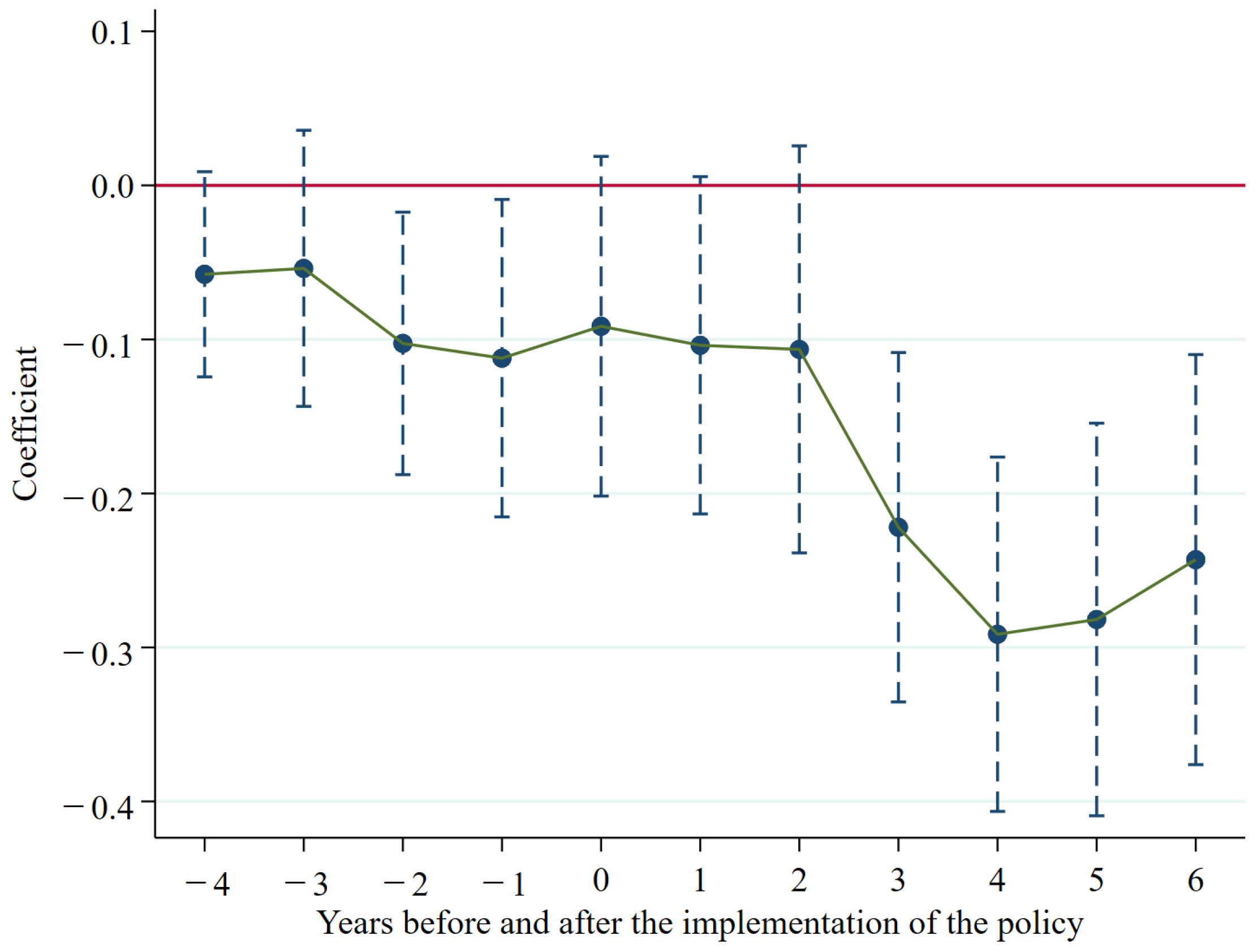
Since the innovation industrial agglomeration pilot (IIAP) policy was proposed in 2013, the range of the pilot has been continuously expanded. On the one hand, the pilot policy stimulates the innovation and development of enterprises; on the other hand, the pilot policy takes the government as the main body. The local government will play a guiding and supervisory role. With regular accessing of the work progress, problems, such as difficulties in resource flow, excessive consumption of raw materials, and increased pollutant emissions encountered during the development of innovative industrial agglomeration, can be solved in time. This study explores the effect of the IIAP on the environment through carbon efficiency and the environmental pollution index. We further develop an in-depth analysis using technological innovation as a mediating variable.

We conclude that the IIAP policy can promote environmentally-friendly development. On the one hand, the implementation of the IIAP policy gathers a large number of high-tech talents and technologies, which can raise the utilization efficiency and reduce emission pollutants. On the other hand, the policy guidance of industrial agglomeration is also a characteristic of China’s development in the agglomeration industry. Behind the implementation of the policy is the government, which supervises the enterprises in the agglomeration area, knows the work situation, and solves the pollution problems in the process of innovation in time. Industrial agglomeration in a particular geographical area is conductive to the centralized disposal of discharged pollutants. Therefore, the IIAP policy can promote environmentally-friendly development. Second, the IIAP policy can indirectly promote environmental-friendly development through technological innovation. Innovative industry agglomeration is knowledge-intensive and technology-intensive and, thus, attracts high-skilled talents. In turn, it improves the technological innovation of enterprises and promotes the efficiency of clean energy research and development, which in turn has a positive effect on environmental. Third, the effect of the IIAP policy on environmentally-friendly development is mainly in the central region, non-resource-based cities, and large cities, with obvious regional differences in distribution. Fourth, there is a spatial siphon effect of the IIAP policy on the environmental pollution index (EPI). The IIAP policy can provide excellent conditions for agglomeration areas and attract the inflow of talents and innovation factors from the surrounding areas. Therefore, it will lead to a decrease in technological innovation in the neighboring areas, which will be detrimental to the environmental improvement in the neighboring areas in the short term.

Our results lead to the following policy implications. Firstly, the government should continue to maintain the steady growth of the pilot units of innovative industrial agglomeration. The IIAP policy has achieved positive effects on environmentally-friendly development. To advance the social effect of the IIAP policy on the environment, the Ministry of Science and Technology of China should steadily promote the construction of innovative industrial agglomeration. It should reasonably plan the cultivation of pilot industries. In the meantime, it should advance the opening of pilot cities in an active and orderly manner, accelerate the development of innovative industries, and contribute to environmentally-friendly development. Secondly, it should actively promote technological innovation capability in the agglomeration region. The local government should further play the leading role in this pilot policy, and adopt tax incentives, financial subsidies, and other forms to actively encourage enterprises to gather innovative technologies and talents. The development of technological innovation level can be accelerated, and the resource utilization efficiency and pollution control rate can be improved, in consequence. Finally, it should optimize the spatial layout of innovative industrial agglomeration. The promotion of the IIAP cities should advocate the development strategy suitable for local conditions, thoroughly combine and utilize the advantages of resources inside and outside the region, and better promote environmentally-friendly development.

Our study must be considered in light of several limitations. Firstly, compared with the low-carbon pilot policy, smart cities pilot policy, and other policies, the IIAP policy in China is not deeply understood by the public. Although the regional scope of the pilot unit has been expanding since its implementation, it still needs to be improved compared with other policies. Secondly, the impact of the IIAP policy on the environment may be through technological innovation, industrial structures, and financial development, etc. This paper examines the effect of the IIAP policy on the environment by using technological innovation as a mediating variable. Technological innovation only serves as a resource transmission path, so a more extensive framework should be constructed in future research to conduct a more profound analysis.

References

1. Alataş, S. The role of information and communication technologies for environmental sustainability: Evidence from a large panel data analysis. J. Environ. Manag. 2021, 293, 112889. [Google Scholar] [CrossRef]
2. Shin, D.; Woodwark, M.J.; Konrad, A.M.; Jung, Y. Innovation strategy, voice practices, employee voice participation, and organizational innovation. J. Bus. Res. 2022, 147, 392–402. [Google Scholar] [CrossRef]
3. Wang, Q.; Qu, J.; Wang, B.; Wang, P.; Yang, T. Green technology innovation development in China in 1990–2015. Sci. Total Environ. 2019, 696, 134008. [Google Scholar] [CrossRef]
4. Ye, J.; Wan, Q.; Li, R.; Yao, Z.; Huang, D. How do R&D agglomeration and economic policy uncertainty affect the innovative performance of Chinese high-tech industry? Technol. Soc. 2022, 69, 101957. [Google Scholar]
5. Liu, Z.; Zeng, S.; Jin, Z.; Shi, J.J. Transport infrastructure and industrial agglomeration: Evidence from manufacturing industries in China. Transp. Policy 2022, 121, 100–112. [Google Scholar] [CrossRef]
6. Yuan, H.; Feng, Y.; Lee, C.C.; Cen, Y. How does manufacturing agglomeration affect green economic efficiency? Energy Econ. 2020, 92, 104944. [Google Scholar] [CrossRef]
7. Wang, X.; Zhang, Q.; Chang, W.Y. Does economic agglomeration affect haze pollution? Evidence from China’s Yellow River basin. J. Clean. Prod. 2022, 335, 130271. [Google Scholar] [CrossRef]
8. Bai, C.; Zhou, L.; Xia, M.; Feng, C. Analysis of the spatial association network structure of China’s transportation carbon emissions and its driving factors. J. Environ. Manag. 2020, 253, 109765. [Google Scholar] [CrossRef]
9. Dong, K.; Ren, X.; Zhao, J. How does low-carbon energy transition alleviate energy poverty in China? A nonparametric panel causality analysis. Energy Econ. 2021, 103, 105620. [Google Scholar] [CrossRef]
10. Speldekamp, D.; Knoben, J.; Saka-Helmhout, A. Clusters and firm-level innovation: A configurational analysis of agglomeration, network and institutional advantages in European aerospace. Res. Policy 2020, 49, 103927. [Google Scholar] [CrossRef]
11. Krugman, P. Increasing Returns and Economic Geography. J. Polit. Econ. 1991, 99, 483–499. [Google Scholar] [CrossRef]
12. Habiba, U.; Cao, X.; Anwar, A. Do green technology innovations, financial development, and renewable energy use help to curb carbon emissions? Renew. Energy 2022, 193, 1082–1093. [Google Scholar] [CrossRef]
13. Ma, Y.; Zhao, H.; Liu, Q. Characteristics of PM2.5 and PM10 pollution in the urban agglomeration of Central Liaoning. Urban. Clim. 2022, 43, 101170. [Google Scholar] [CrossRef]
14. Fu, Y.; He, C.; Luo, L. Does the low-carbon city policy make a difference? Empirical evidence of the pilot scheme in China with DEA and PSM-DID. Ecol. Indic. 2020, 122, 107238. [Google Scholar] [CrossRef]
15. Xie, R.; Fu, W.; Yao, S.; Zhang, Q. Effects of financial agglomeration on green total factor productivity in Chinese cities: Insights from an empirical spatial Durbin model. Energy Econ. 2021, 101, 105449. [Google Scholar] [CrossRef]
16. Shen, N.; Peng, H. Can industrial agglomeration achieve the emission-reduction effect? Socio-Econ. Plan. Sci. 2020, 75, 100867. [Google Scholar] [CrossRef]
17. Liu, J.; Cheng, Z.; Zhang, H. Does industrial agglomeration promote the increase of energy efficiency in China? J. Clean. Prod. 2017, 164, 30–37. [Google Scholar] [CrossRef]
18. Gu, Q.; Wang, H.; Zheng, Y.; Zhu, J.; Li, X. Ecological footprint analysis for urban agglomeration sustainability in the middle stream of the Yangtze River. Ecol. Modell. 2015, 318, 86–99. [Google Scholar] [CrossRef]
19. Yu, X.; Geng, Y.; Dong, H.; Fujita, T.; Zhe, L. Emergy-based sustainability assessment on natural resource utilization in 30 Chinese provinces. J. Clean. Prod. 2016, 133, 18–27. [Google Scholar] [CrossRef]
20. Wen, Y.; Liao, M.; Siddiqui, M.M. The impact of industrial agglomeration on carbon emissions: Empirical evidence from China. Int. J. Manag. Sustain. 2019, 8, 67–78. [Google Scholar] [CrossRef]
21. Bechara, C.A.; Alnouri, S.Y. Energy assessment strategies in carbon-constrained industrial clusters. Energy Convers. Manag. 2022, 254, 115204. [Google Scholar] [CrossRef]
22. Chen, C.; Sun, Y.; Lan, Q.; Jiang, F. Impacts of industrial agglomeration on pollution and ecological efficiency-A spatial econometric analysis based on a big panel dataset of China’s 259 cities. J. Clean. Prod. 2020, 258, 120721. [Google Scholar] [CrossRef]
23. Wu, D.; Wang, Z.; Chen, J.; Kong, S.; Fu, X.; Deng, H.; Shao, G.; Wu, G. Aromatic hydrocarbons (PAHs) in atmospheric PM2.5 and PM10 at a coal-based industrial city: Implication for PAH control at industrial agglomeration regions, China. Atmos. Res. 2014, 149, 217–229. [Google Scholar] [CrossRef]
24. Han, F.; Xie, R.; Lu, Y.; Fang, J.; Liu, Y. The effects of urban agglomeration economies on carbon emissions: Evidence from Chinese cities. J. Clean. Prod. 2018, 172, 1096–1110. [Google Scholar] [CrossRef]
25. Dong, F.; Wang, Y.; Zheng, L.; Li, J.; Xie, S. Can industrial agglomeration promote pollution agglomeration? Evidence from China. J. Clean. Prod. 2020, 246, 118960. [Google Scholar] [CrossRef]
26. Ang, J.B. CO2 emissions, energy consumption, and output in France. Energy Policy 2007, 35, 4772–4778. [Google Scholar] [CrossRef]
27. Huang, C.; Wang, J.W.; Wang, C.M.; Cheng, J.H.; Dai, J. Does tourism industry agglomeration reduce carbon emissions? Environ. Sci. Pollut. Res. 2021, 28, 1–6. [Google Scholar] [CrossRef]
28. Tang, P.; Yang, S.; Shen, J.; Fu, S. Does China’s low-carbon pilot programme really take off? Evidence from land transfer of energy-intensive industry. Energy Policy 2018, 114, 482–491. [Google Scholar] [CrossRef]
29. Hu, Y.J.; Li, X.Y.; Tang, B.J. Assessing the operational performance and maturity of the carbon trading pilot program: The case study of Beijing’s carbon market. J. Clean. Prod. 2017, 161, 1263–1274. [Google Scholar] [CrossRef]
30. Cheng, J.; Yi, J.; Dai, S.; Xiong, Y. Can low-carbon city construction facilitate green growth? Evidence from China’s pilot low-carbon city initiative. J. Clean. Prod. 2019, 231, 1158–1170. [Google Scholar] [CrossRef]
31. Li, X.; Lai, X.; Zhang, F. Research on green innovation effect of industrial agglomeration from perspective of environmental regulation: Evidence in China. J. Clean. Prod. 2021, 288, 125583. [Google Scholar] [CrossRef]
32. Zhang, Y.; Wang, S. Influence of marine industrial agglomeration and environmental regulation on marine innovation efficiency—From an innovation value chain perspective. Mar. Policy 2021, 134, 104807. [Google Scholar] [CrossRef]
33. Shuo, C.; Anna, S.; Xin, W. Carbon emission curbing effects and influencing mechanisms of China’s Emission Trading Scheme: The mediating roles of technique effect, composition effect and allocation effect. J. Clean. Prod. 2020, 264, 121700. [Google Scholar]
34. Huo, W.; Qi, J.; Yang, T.; Liu, J.; Liu, M.; Zhou, Z. Effects of China’s pilot low-carbon city policy on carbon emission reduction: A quasi-natural experiment based on satellite data. Technol. Forecast. Soc. Chang. 2022, 175, 121422. [Google Scholar] [CrossRef]
35. Yu, Y.; Chen, X.; Zhang, N. Innovation and energy productivity: An empirical study of the innovative city pilot policy in China. Technol. Forecast. Soc. Chang. 2022, 176, 121430. [Google Scholar] [CrossRef]
36. Liu, X.; Zhang, X. Industrial agglomeration, technological innovation and carbon productivity: Evidence from China. Resour. Conserv. Recycl. 2021, 166, 105330. [Google Scholar] [CrossRef]
37. Li, C.; Qi, Y.; Liu, S.; Wang, X. Do carbon ETS pilots improve cities’ green total factor productivity? Evidence from a quasi-natural experiment in China. Energy Econ. 2022, 108, 105931. [Google Scholar] [CrossRef]
38. Pastor, J.T.; Lovell, C.A.K. A global Malmquist productivity index. Econ. Lett. 2005, 88, 266–271. [Google Scholar] [CrossRef]
39. Meng, M.; Qu, D. Understanding the green energy efficiencies of provinces in China: A Super-SBM and GML analysis. Energy 2022, 239, 121912. [Google Scholar] [CrossRef]
40. Gumbau-Albert, M.; Maudos, J. Patents, technological inputs and spillovers among regions. Appl. Econ. 2009, 41, 1473–1486. [Google Scholar] [CrossRef]
41. Zhu, B.; Zhang, M.; Huang, L.; Wang, P.; Su, B.; Wei, Y.M. Exploring the effect of carbon trading mechanism on China’s green development efficiency: A novel integrated approach. Energy Econ. 2020, 85, 104601. [Google Scholar] [CrossRef]
42. Beck, T.; Levine, R.; Levkov, A. Big Bad Banks? The Winners and Losers from Bank Deregulationin the United States. J. Financ. Econ. 2010, 65, 1637–1667. [Google Scholar]
43. Baron, R.M.; Kenny, D.A. The moderator–mediator variable distinction in social psychological research: Conceptual, strategic, and statistical considerations. J. Pers. Soc. Psychol. 1986, 51, 1173. [Google Scholar] [CrossRef] [PubMed]
44. Jacobson, L.S.; Sullivan, L. Earnings Losses of Displaced Workers. Am. Econ. Rev. 1993, 83, 685–709. [Google Scholar]
45. Yang, X.; Lin, S.; Li, Y.; He, M. Can high-speed rail reduce environmental pollution? Evidence from China. J. Clean. Prod. 2019, 239, 118135. [Google Scholar] [CrossRef]
46. Sun, L.; Li, W. Has the opening of high-speed rail reduced urban carbon emissions? Empirical analysis based on panel data of cities in China. J. Clean. Prod. 2021, 321, 128958. [Google Scholar] [CrossRef]
47. Yang, Q.; Gao, D.; Song, D.; Li, Y. Environmental regulation, pollution reduction and green innovation: The case of the Chinese Water Ecological Civilization City Pilot policy. Econ. Syst. 2021, 45, 100911. [Google Scholar] [CrossRef]
48. Wang, J.; Yang, N.; Zhang, Y.; Song, Y. Dynamics of firm’s network community associations and firm’s innovation performance. Technol. Anal. Strateg. Manag. 2022, 32, 239–255. [Google Scholar] [CrossRef]
49. Yan, J.; Zhao, J.; Yang, X.; Su, X.; Wang, H.; Ran, Q.; Shen, J. Does Low-Carbon City Pilot Policy Alleviate Urban Haze Pollution? Empirical Evidence from a Quasi-Natural Experiment in China. Int. J. Environ. Res. Public Health 2021, 18, 11287. [Google Scholar] [CrossRef]
50. Feng, Y.; Wang, X. Effects of urban sprawl on haze pollution in China based on dynamic spatial Durbin model during 2003–2016. J. Clean. Prod. 2020, 242, 118368. [Google Scholar] [CrossRef]
51. Chagas, A.L.S.; Azzoni, C.R.; Almeida, A.N. A spatial difference-in-differences analysis of the impact of sugarcane production on respiratory diseases. Reg. Sci. Urban. Econ. 2016, 59, 24–36. [Google Scholar] [CrossRef]
52. Ke, S.; Feser, E. Count on the Growth Pole Strategy for Regional Economic Growth? Spread–Backwash Effects in Greater Central China. Reg. Stud. 2010, 44, 1131–1147. [Google Scholar] [CrossRef]
53. Feng, Y.; Wang, X.; Liang, Z.; Hu, S.; Xie, Y.; Wu, G. Effects of emission trading system on green total factor productivity in China: Empirical evidence from a quasi-natural experiment. J. Clean. Prod. 2021, 294, 126262. [Google Scholar] [CrossRef]
54. Shan, Y.; Guan, Y.; Hang, Y.; Zheng, H.; Li, Y.; Guan, D.; Li, J.; Zhou, Y.; Li, L.; Hubacek, K. City-level emission peak and drivers in China. Sci. Bull. 2022, 67, 1910–1920. [Google Scholar] [CrossRef]
Figure 1. Parallel trend test (EPI). The vertical dashed line indicates the 95% confidence interval.
Sustainability 14 13571 g001
Figure 2. Placebo test. Subfigure (a) shows the placebo test results for CEE, and subfigure (b) shows the placebo test results for EPI.
Sustainability 14 13571 g002
Figure 3. Kernel density function matching. Subfigure (a) shows the results of the kernel density distribution between the treatment and control groups before using the PSM method, and subfigure (b) shows the results after using the PSM method.
Sustainability 14 13571 g003