Safety and Sustainable Development of Automated Driving in Mixed-Traffic Urban Areas—Considering Vulnerable Road Users and Network Efficiency

Abstract

Next to environmental aspects, establishing areas for safe and economically viable automated driving in mixed-traffic settings is one major challenge for sustainable development of Autonomous Vehicles (AVs). This work investigates safety in the interactions between AVs, human-driven vehicles, and vulnerable road users, including cyclists and pedestrians, within a simulated urban environment in the Dutch city of Rotterdam. New junction and pedestrian models are introduced, and virtual AVs with an occlusion-aware driving system are deployed to deliver cargo autonomously. The safety of applying this autonomous cargo delivery service is assessed using a large set of Surrogate Safety Indicators (SSIs). Furthermore, Macroscopic Fundamental Diagrams (MFDs) and travel time loss are incorporated to evaluate the network efficiency. By assessing the impact of various measures involving Vehicle-to-Vehicle (V2V), Vehicle-to-Infrastructure (V2I), Vehicle-to-Everything (V2X) communications, infrastructure modifications, and driving behavior, we show that traffic safety and network efficiency can be achieved in a living lab setting for the considered case. Our findings further suggest that V2X gets implemented, new buildings are not placed close to intersections, and the speed limit of non-arterial roads is lowered.

1. Introduction

Autonomous Vehicles (AVs) are anticipated to bring a transition with a significant impact on the transportation sector. It is generally accepted that the potential benefits of deploying these vehicles are increased road capacity, traffic safety, and driving comfort. Companies like Waymo, Tesla, GM Cruise, Baidu, and Argo AI are working on driverless technologies, and some of them are so far in development that they claim to drive safer than humans [1]. Nonetheless, establishing areas for safe and efficient automated driving in mixed-traffic settings is one major challenge for the sustainable development and adoption of AVs. Next to environmental sustainability, social and economic sustaintainbility particularly considering the interaction between AVs, infrastructure, conventional vehicles, and vulnerable road users (VRUs) such as pedestrians can be studied in urban living labs. In this context, VRUs are understood to be non-motorized road users such as pedestrians and cyclists as well as motor-cyclists and persons with disabilities.

The former port area of the Merwe- and Vierhavensgebied (M4H) in the Dutch city of Rotterdam is currently transformed into a vibrant new part of the city where new manufacturing industries, urban facilities, housing, and culture come together [2]. It is believed that autonomous freight transport could play a part in these new manufacturing industries in the near future.

This work addresses the gap in knowledge on the impact of introducing AVs in urban networks concerning traffic safety and network efficiency for all road users and how to mitigate the potential negative effects. A simulated scenario applying AVs, human-driven vehicles, and Vulnerable Road Users (VRUs), based on the case of the M4H area in Rotterdam, is created. Then, this mixed traffic urban network is assessed on its safety with a large set of Surrogate Safety Indicators (SSIs), and its network efficiency is evaluated with Macroscopic Fundamental Diagrams (MFDs) and a travel time loss analysis. SSIs describe the closeness to or the severity of a collision between two entities in an objective way. To ensure AVs safety and realistic behavior at all times, the AVs in this research consider a limited sensorial view with the Occlusion Aware Driving (OAD) principle. We further investigate the impact of various measures involving Vehicle-to-Vehicle (V2V), Vehicle-to-Infrastructure (V2I), Vehicle-to-Everything (V2X) communications, infrastructure modifications, and driving behavior on network safety and efficiency.

The remainder of the paper is structured as follows. In Section 2, the related literature is briefly reviewed, and the existing gaps are identified. Section 3 describes the proposed urban traffic safety assessment approach. Section 4 deals with evaluating urban traffic efficiency assessment. In Section 5, the developed applied OAD framework is introduced. The case study, results, and discussions are presented in Section 6. We further outline policy implications of this work in Section 7. Finally, the paper is concluded in Section 8, and future research directions are proposed.

2. Related Work

This research mainly contributes to two branches of literature: Safety assessment for simulated environments and operational efficiency evaluation, which will be briefly reviewed in this section.

2.1. Safety Assessment

In combination with the Surrogate Safety Indicator (SSI) assessment, microsimulation has proven to be a reliable prediction method for collision risk. Mahmud et al. [3] and Johnsson et al. [4] did comprehensive work reviewing SSI research developments and provided an overview of existing SSIs and their performance. Johnsson et al. [4] focused on indicators that apply to VRUs, for which SSI research is limited.

A lot of traffic safety research works have already been conducted using SSIs. In the work of Guido et al. [5], historical collision data were found to match with collision data coming from a microscopic simulation, which was analyzed using SSIs. Virdi et al. [6] investigated how market penetration of Connected Vehicles (CV) impact safety in a mixed urban and highway situation. They showed that at 90% CV market penetration, the number of conflicts at signalized, priority, roundabout, and diverging diamond intersections are accompanied by −48%, −100%, −98%, and −81% changes, respectively. Essa and Sayed [7] calibrated a microscopic simulation model using a genetic algorithm to match the vehicles’ actual behavior. Conflict heat maps were generated to compare field-measured with simulated conflict locations.

Li et al. [8] used the Swedish Traffic Conflict Technique (STCT) to identify and analyze video footage conflicts. Using the Time-to-Collision (TTC) SSI, they estimated the Hourly Composite Risk Indexes (HCRI) of the real network with the simulated data by tuning the influencing parameters. The STCT, in combination with a microscopic simulator, was used by Axelsson and Wilson [9] to investigate the traffic safety of an intersection in the city center of Stockholm. They concluded that with the differences between field observations and simulation evaluation methods in mind, the simulation method can still be used to indicate the level of traffic safety.

Tafidis et al. [10] mentioned that existing research is mainly focused on operational efficiency and safety gains of the AVs without considering VRUs. In their work, safety and network performance while introducing AVs and cyclists were studied. They concluded that AVs’ introduction in the road network reduced the number and severity level of cyclist-vehicle conflicts. Another approach to assess traffic safety is taken by Fancello et al. [11]. Using a set of subjective and objective indicators, they performed a multiple-criteria decision analysis (VIKTOR and TOPSIS) to rank individual intersections on safety, with which a plan of priority interventions to improve road safety can be specified.

Table 1. Literature table of urban safety assessment studies.

Study	Safety Evaluation Method			Considered Vehicle Types				Study Area		Data Obtained by
	SSI	AD	MS	AV	CV	BK	PD	UR	HW	SM	RL
[5]	✓	✓			✓			✓		✓	✓
[6]	✓		✓	✓	✓			✓	✓	✓
[7]	✓				✓			✓		✓	✓
[8]	✓	✓			✓			✓		✓	✓
[9]	✓	✓	✓	✓	✓	✓	✓	✓		✓	✓
[10]	✓		✓	✓	✓	✓		✓		✓
[11]		✓			✓		✓	✓			✓
[12]	✓	✓		✓	✓			✓		✓	✓
This research	✓		✓	✓	✓	✓	✓	✓		✓
SSI	Surrogate safety indicators			CV	Conventional vehicles			HW	Highway
AD	Actual crash data			BK	Bikes			SM	Simulation
MS	Multiple scenarios			PD	Pedestrians			RL	Real network
AV	Autonomous vehicles			UR	Urban

provides a brief overview of the literature on safety evaluation.

2.2. Operational Efficiency

Budan et al. [13] investigated the impact of introducing connected autonomous vehicles at signalized intersections on operational performance. They concluded that at low congestion, First-Come-First-Served (FCFS) scheduling reduces fuel consumption, average time loss, and queue length. At higher congestion states, actuated traffic lights outperform the FCFS scheduling procedure.

Wang et al. [14] researched the effect of autonomous driving in urban environments by representing AVs as vehicles with Adaptive Cruise Control (ACC) and cooperative ACC. It was concluded that the performance increase in urban environments is significantly lower compared to highway environments. Using an urban grid network with actuated traffic lights, Lu and Tettamanti [15] generated the MFD for six market penetration situations with a mixed fleet of autonomous vehicles. The results justified some regularity in the change of the urban MFD. In later research [16], they also considered a real network alongside the grid network and varied the market penetration. The resulting MFDs from both networks showed a quasi-linear increase in network capacity with increasing market penetration rates. Furthermore, digital transportation platorms [17] are increasingly considering AVs to leverage unused vehicles in cities [18] and provide customers with a high-quality mobility services [19]. The literature on urban operational efficiency-related work is presented in

Table 2. Literature table of urban safety assessment studies.

Study	Efficiency Evaluation Method			Performance Measures				Considered Vehicle Types
	TT	FC	FD	IF	TM	VC	PR	AV	CV	BK	PD
[10]	✓							✓	✓	✓
[13]	✓	✓		✓	✓	✓		✓	✓
[14]			✓			✓	✓	✓	✓
[15]	✓		✓					✓	✓
[16]	✓		✓					✓	✓
This research	✓		✓	✓		✓		✓	✓	✓	✓
TT	Travel time loss			TM	Traffic management			CV	Conventional vehicles
FC	Fuel consumption			VC	Vehicle communication			BK	Bikes
FD	Fundamental diagram			PR	Prediction			PD	Pedestrians
IF	Infrastructure			AV	Autonomous vehicles

.

2.3. Existing Gap

The review of the literature reveals two main research gaps in the area, which are listed as follows:

• There is no combined urban microscopic simulation framework with AVs, human-driven vehicles, and VRUs (bikes and pedestrians) to assess safety and operational efficiency.
• There is no overview of the influence of various measures taken to improve safety and operational efficiency in urban mixed-traffic (including VRUs) situations.

These research gaps are filled by proposing a framework in which virtual AVs can be injected into the microscopic traffic simulator SUMO and assessed in terms of safety and operational efficiency. In the simulated network, trailers, cars, bikes, and pedestrians are present. The AVs use an Occlusion Aware Driving (OAD) principle. Although this driving principle is perfectly safe in simulated scenarios, it is also very conservative. To mitigate this, the impact of several countermeasures is investigated by simulating the network under various scenarios.

3. Urban Traffic Safety Assessment

Traditionally, road safety is measured by crash rates and the severity of these crashes. Although the approach is well-established, it faces four significant concerns. Firstly, the relative infrequency and unpredictability of accidents result in small sample sizes, often lacking details regarding failure mechanisms and crash avoidance behavior [3,4,20]. Secondly, more severe accidents are more likely to be reported, while small accidents, often involving VRUs, are less likely to be reported [21,22]. Thirdly, near misses and uncomfortable driving situations are expected not to be reported because they are not severe enough. Lastly, ethical problems associated with long-term data collection without taking intermediate actions exist [3].

The traditional approach to measure road safety only considers data acquired from accidents. Another method is the quantitative measurement of safety with Surrogate Safety Indicators (SSIs), in which surrogate implies that incident data are utilized instead of accident data [4]. This method provides objective data, which is based on closeness to a collision. This closeness can be grouped into temporal, distance-based, and deceleration-based; there are also some miscellaneous indicators. For SSIs to be useful, there should be a relation between the indictors, crash rate, and severity. The process of determining SSIs is often automated using video analysis tools, as was demonstrated by Saunier and Sayed [23], which allows rich data sets to be collected. Ideally, there is a linear correlation between the SSI, severity, and/or crash rate [4]. It is important to note that there are typically no set thresholds that determine whether a situation is safe or unsafe. When it is impossible to correlate the indicator’s value to an hourly crash rate or crash severity, the data becomes more abstract but can still indicate the amount of safety slack in events.

There exist different SSIs in the literature; among those, the following are the mostly applied ones that fit into this research.

Time-To-Collision (TTC): TTC is defined as the time left until an accident between two vehicles occurs if they do not alter their trajectory or velocity [24]. TTC is calculated as follows, where $\mathsf{\Delta }{X}_{i,j}$ is the bumper to the bumper distance between two vehicles, and $\mathsf{\Delta }{V}_{i,j}$ is the relative velocity:

$$TT{C}_i\left(t\right)=\frac{\Delta X_{i,j}\left(t\right)}{\Delta V_{i,j}\left(t\right)}$$

(1)

and the $TT{C}_{span}$ is:

$$TT{C}_{i,span}=\left[\begin{array}{c}TTC\left(t_0\right)\\ TTC\left(t_1\right)\\ ⋮\\ TTC\left(t_n\right)\end{array}\right]$$

(2)

where $t_0$ is the starting point of the conflict and $t_n$ is the endpoint. Since a lower TTC increases the chance of collision, often the minimum known as TTC_min is subjected to a TTC threshold (TTC*) value. If the TTC is lower than the TTC*, the incident is reported as critical.

Time-to-Accident (TA): TA is the TTC value when an entity takes action to avoid a collision [25]. The advantage of using TA over TTC_min is that the safety level at the time an evasive action takes place is recorded instead of during or at the end of the evasive action.

Time Integrated Time-to-Collision (TIT): TIT takes the integral of the TTC profile and expresses the level of unsafety in ${\mathrm{s}}^2$. This way, the time an entity spends in a safety-critical situation and the amount TTC is lower than TTC* are considered. As long as the TTC remains below the threshold, the area between the TTC* and the TTC is calculated.

Modified Time-To-Collision (MTTC): TTC assumes that both vehicles keep the same speed, and the current acceleration or deceleration is not considered. This neglects the evasive action that is already being taken by the entities. MTTC is introduced by Ozbay et al. [26] to overcome this challenge. It takes the relative distance, relative speed, and relative acceleration into account and better represents the actual time until a collision occurs compared to TTC.

Crash Index (CI): CI is based on kinetics’ idea to consider the effect of speed on the kinetic energy at impact [16]. This SSI gives an indication of the severity of conflict based on MTTC. A shortcoming of this approach is that it neglects the entities’ mass as it assumes that different vehicle types do not differ much in mass.

The Post-Encroachment Time (PET): PET indicates the time difference between an offending vehicle leaving the conflict area and the arrival time of a vehicle that possesses the right of way [27]. PET is considered a robust indicator since it only requires two points in time, and unlike most TTC-based indicators, does not rely on arrival time estimations.

Proportion of Stopping Distance (PSD): PSD is defined as the ratio between the remaining stopping distance and minimum stopping distance [27]. If the value is below 1, there is not enough room to stop before reaching the conflict point.

Deceleration Rate to Avoid the Crash (DRAC): DRAC, as introduced by Almqvist et al. [28] is the speed differential ratio between leader and follower and their closing time. A DRAC value greater than the emergency deceleration is considered critical.

Criticality index Function (CrF): CrF, as proposed by Ching-Yao [29], is based on two principles. Firstly, the higher the collision speed, the more severe the crash would be. Secondly, the longer the TTC, the more time to execute an evasive action is available. With these two principles in mind, CrF is defined as the squared speed of the oncoming vehicle divided by the TTC.

Pedestrian Risk Index (PRI): PRI is a combined indicator for risk and severity of vehicle-pedestrian conflicts on zebra crossings introduced by Cafiso et al. [30], which has been used by several researchers later. PRI combines the Time-to-Zebra (TTZ), which is the TTC but with zero speed for the pedestrian, with assumptions about reaction time and deceleration capability [4]. The PRI considers the duration of the conflict, the reaction time and braking capability of the vehicle, the degree of safety, and impact speed.

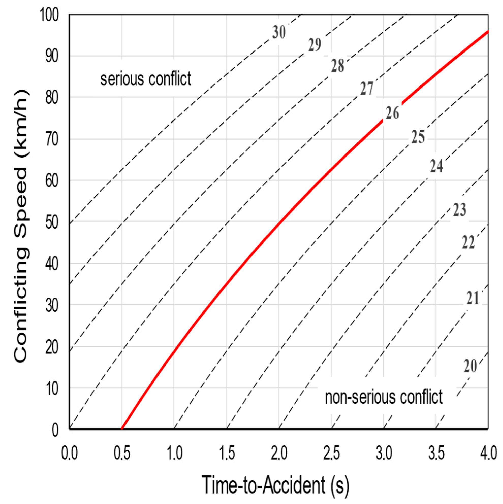
Swedish Traffic Conflict Technique (STCT): STCT can be used to identify and classify traffic conflicts based on TA and Conflicting Speed (CS), which is the vehicle’s speed when it takes evasive action. Figure 1 shows the relation between seriousness, CS, and TA. This graph is used to determine the level of severity of an incident. If TA increases, the seriousness decreases as there is more time to execute the evasive action. If the CS increases, the required time to execute an evasive action increases, and thereby the seriousness increases. When the level of severity is above 26, the conflict is considered serious [31]. There is a strong statistical relation between police-reported accidents and serious conflicts [32]. In this case, the seriousness level of the STCT is used as an SSI.

Due to its simplicity and objectivity, the Swedish TCT is the most well-known TCT, but several alternative techniques from other countries do exist: the Austrian [33], Canadian [34], Czech [35], Dutch [36], Finnish [37], French [38], German [39], British [40] and American [41] TCT. Most of these are old and not as actively maintained as the STCT, or they are (partly) based on expert opinion. The alternative techniques are well documented in the literature, and further addressing them is out of the scope of this research.

4. Urban Traffic Efficiency Assessment

4.1. Macroscopic Fundamental Diagrams

Macroscopic Fundamental Diagrams (MFDs) describe the relation between traffic density, flow, and average speed and are widely used as a tool in the design process of highway road networks [43] together with the description of the mentioned relation in urban networks. A typical MFD consists of a set of three plots: density-flow, density-speed, and speed-flow. All plots are related to the fundamental relationship:

$$Q=V·\rho$$

(3)

where Q denotes the flow [vehicles·h⁻¹], V the average speed [km·h⁻¹] and ρ the vehicle density [vehicles·km⁻¹].

4.2. Time Loss

Aside from MFDs, time loss (or delay) is often used as a measure of efficiency. Where MFDs describe the network level’s performance over the entire congestion spectrum, time loss describes the performance on a vehicular level at a particular level of service. A benefit of using time loss is that it is easier to understand and can be calculated per vehicle type. While MFDs are rather abstract and always consider all entities in (a part of) the network or on a lane. When using time loss as an indicator for operational performance, it is essential to constantly have the same service level (for instance, the same injection rate of vehicles) in these comparison cases.

5. Occlusion Aware Driving Model

What distinguishes this research from comparable microscopic traffic studies is the Occlusion Aware Driving (OAD) principle. The AVs are modeled such that their visibility range gets obstructed by obstacles such as buildings. Because of high computing power requirements, view obstructions caused by other road users are not considered.

OAD considers imaginary entities (Pseudo Vehicles (PVs)) at the visibility range border instead of only considering visible entities. There are two types of PVs: static PVs, which are modeled as a vehicle with zero speed and no intention to drive off, and dynamic PVs, which are modeled as the vehicles that drive the maximum allowed lane speed and have no intention to brake. This way, the AV should never be overwhelmed if an entity that was previously behind an occlusion appears, and safety is guaranteed.

Lin et al. [44] used a similar OAD approach. In their work, decisions on junctions are made with a Partially Observable Markov Decision Process (POMDP). It is common practice to use POMDP as a decision-making algorithm in autonomous driving models [45,46]. However, due to the high number of interactions in this use case, it was not feasible to use the POMPD as it uses a lot of computational resources. Therefore, in this work, a simplified rule-based model was applied.

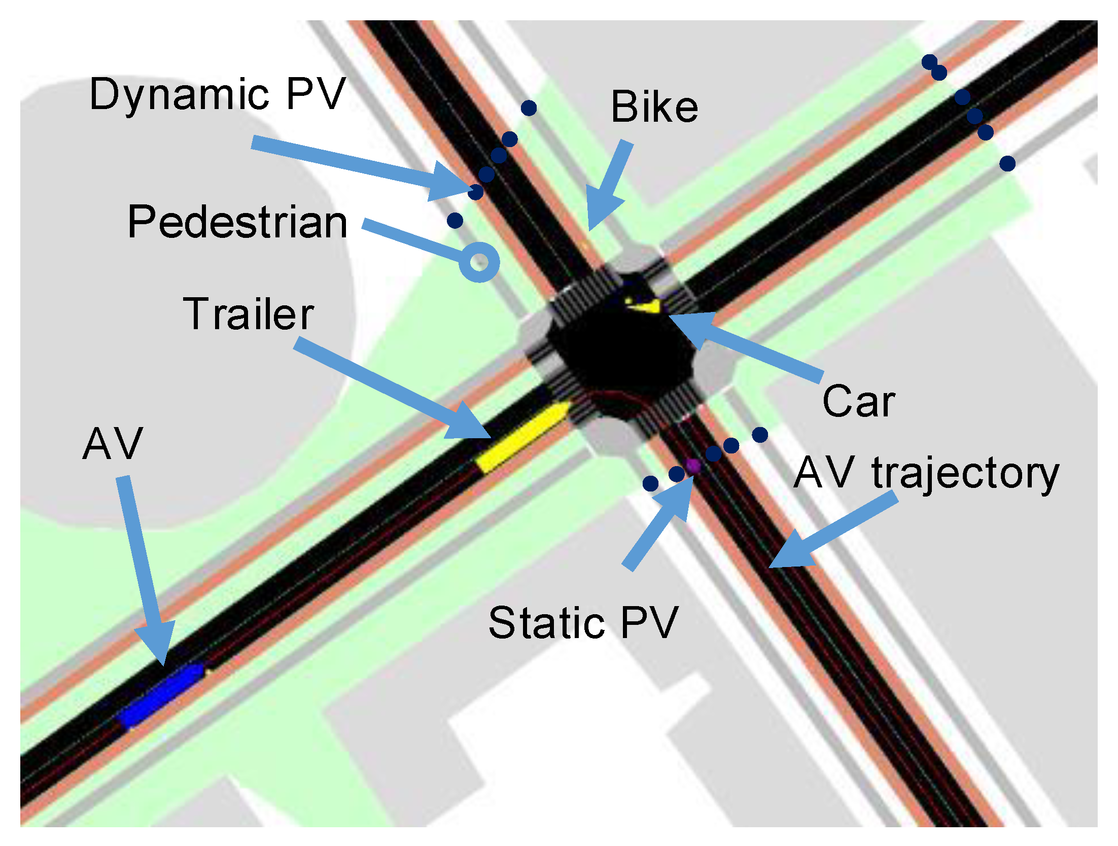
In Figure 2, an AV in the simulation is shown with all relevant elements indicated. Generally, only one static PV on the AV trajectory is considered, but several dynamic PVs are present. A dynamic PV is not just one entity with one route, but all possible routes allowed to be taken need to be considered by the AV speed controller logic.

5.1. AV Speed Controller Logic

To control the speed of the AVs, the AV speed controller is introduced. Lane-keeping, steering, and determining the next position of the AV are managed by SUMO, and the speed of AVs is controlled by the speed controller logic. As the decisions by the default model are made centrally rather than locally by the vehicle, it is not possible to implement the OAD by modifying the default models. Therefore, this new speed controller logic is introduced.

The new model calculates the AV’s (together with other cars, trailers, and bikes) safe speed based on three models: car-following model, junction model, and pedestrian model. When the safe speeds for all entities are calculated, the speed controller takes the minimum calculated speed and instructs the AV to accelerate, decelerate, or hold its speed. It also takes the maximum AV and allowed road speed into consideration.

5.1.1. Car-Following Model

The task of the car-following model is to prevent collisions with leading vehicles in the following situations. It does this by keeping a constant time gap ($\tau$) from the leading vehicle. Various car-following models are available in SUMO, an overview of which is available on the SUMO wiki [47]. The Krauß car-following model [48] is chosen for this application, as it is a robust car-following model and was previously used by various researchers, including [49,50]. The safe speed of the vehicle in the next simulation step is calculated by Equation (4). The bumper-to-bumper gap is determined by drawing the AV trajectory and measuring the segments’ length between the AV and the leading vehicle. The leading vehicle’s speed is assumed to be available.

$$v_{saf{e}_{cf},vehicl{e}_n}=v_{vehicl{e}_n}+\frac{g_{AV,vehicl{e}_n}-v_{vehicl{e}_n}·{\tau }_{AV}}{\frac{v_{AV}+v_{vehicl{e}_n}}{2·b_{AV}}+{\tau }_{AV}}$$

(4)

where:

$v_x$: Speed of $x$ [m·s⁻¹]

$g_{x,y}$: Gap between $x$ and $y$ [m]

${\tau }_x$: Time gap of $x$ [s]

$b_x$: Maximum deceleration rate of $x$ [m·s⁻²]

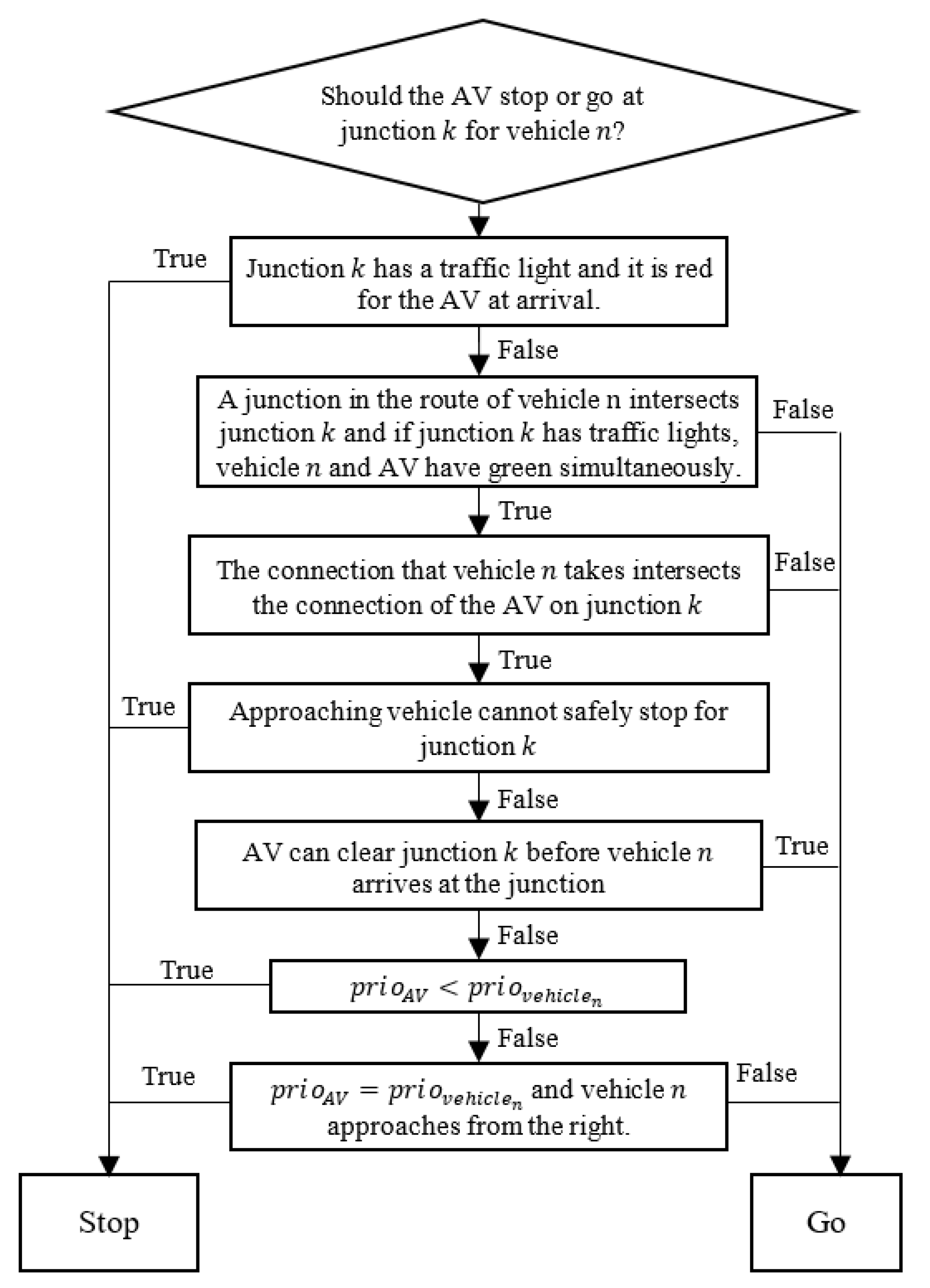
5.1.2. Junction Model

The junction model manages the behavior of the AV when approaching an intersection. The difference between this junction model and the standard model in SUMO is that this logic is from the AV’s perspective, whereas the SUMO model is created from the junction’s perspective. As the decisions by the default junction model are made from the junction’s point of view, it acts more like a junction with actuated traffic lights, whereas the new junction allows the vehicles to make their own choices. Compared to the similar work of Tafidis et al. [10], which uses the default SUMO model, it is believed that this approach results in more realistic behavior of the AVs.

The decision scheme, shown in Figure 3, is the main logic behind the junction model. This logic must be followed for each disturbance vehicle and all intersections in the breaking distance range of the AV as long as the previous intersection’s outcome is “go”. If the outcome for junction k and vehicle n is “stop”, the safe speed of the AV concerning junction k is set to the maximum safe speed to brake in time, and subsequent junctions do not have to be checked. The maximum safe speed for the AV to brake in time for junction k is calculated using Equation (5) (simplified Krauß method). Note that the junction approaching speed is influenced by the desired time gap (${\tau }_{AV}$) of the AV.

$$v_{brakin{g}_{jk}}=\frac{g_{jk,AV}-minGa{p}_{jk}}{\frac{v_{AV}}{2·b_{AV}}+{\tau }_{AV}}$$

(5)

where: $minGa{p}_{jk}$: Minimum gap between AV and junction [m].

Equations (6) to (8) are used to obtain values required for estimating the arrival time of vehicle $n$ at junction $k$. First, the speed difference between the current speed and allowed lane speed is calculated by Equation (6).

$$\Delta v=v_{allowed}-v_x$$

(6)

where: $v_{allowed}$: Maximum allowed speed at approaching lane [m·s⁻¹].

Equation (7) determines the time it takes to accelerate or decelerate to reach this new speed.

$$t_{acc}=\{\begin{array}{c}\frac{\Delta v}{a_x},\Delta v>0\\ \frac{\Delta v}{b_x},\Delta v\le 0\end{array}$$

(7)

where: $a_x$: Maximum acceleration rate of $x$ [m∙s⁻²].

Acceleration or deceleration distance is calculated by Equation (8). This is necessary to determine whether the vehicle is done with accelerating or decelerating before it reaches the junction.

$$s_{acc}=\{\begin{array}{c}{v}_x{t}_{acc}+\frac{a_x{t}_{acc}^2}{2},\Delta v>0\\ v_x{t}_{acc}-\frac{d_x{t}_{acc}^2}{2},\Delta v\le 0\end{array}$$

(8)

Then, the approximated arrival time at junction $k$ is calculated using Equation (9).

$$t_{arrival}=\{\begin{array}{c}\hspace{1em}\hspace{1em}\hspace{1em}\frac{g_{jk,x}-s_{acc}}{v_{allowed}}+t_{acc},|g_{jk,x}-s_{acc}\ge 0\\ max\left(\frac{-v_x\pm \sqrt{v_x^2+2a{g}_{jk,x}}}{a}\right),|g_{jk,x}-s_{acc}<0and\Delta v>0\\ max\left(\frac{v_x\pm \sqrt{v_x^2-2d{g}_{jk,x}}}{d}\right),|g_{jk,x}-s_{acc}<0and\Delta v\le 0\end{array}$$

(9)

where: $g_{jk,x}$ The gap between junction $k$ and $x$ [m].

These calculations can only be used if there are no other junctions between vehicle $n$ and junction $k$ or if the maximum allowed lane speed for all lanes on the trajectory is the same. If this is not the case, the arrival time for junction $k+1$ is calculated by first calculating the end speed ($v_{end}$) at junction $k$ and setting $v_x$ to this value. Note that $g_{jk+1,x}$ needs to be set to the length of the approaching lane of junction $k+1$ plus the connection length at junction $k$. To calculate the clear junction time ($t_{clear}$), the same calculations can be used with the connection length at junction k and the vehicle length added to $g_{jk,x}$.

Finally, the speed at the end of the given gap is calculated by Equation (10).

$$v_{end}=\{\begin{array}{c}{v}_{allowed},|g_{jk,x}-s_{acc}\ge 0\\ –t_{arrival}*a_x+v_x,|g_{jk,x}-s_{acc}<0and\Delta v>0\\ -t_{arrival}*b_x+v_x,|g_{jk,x}-s_{acc}<0and\Delta v\le 0\end{array}$$

(10)

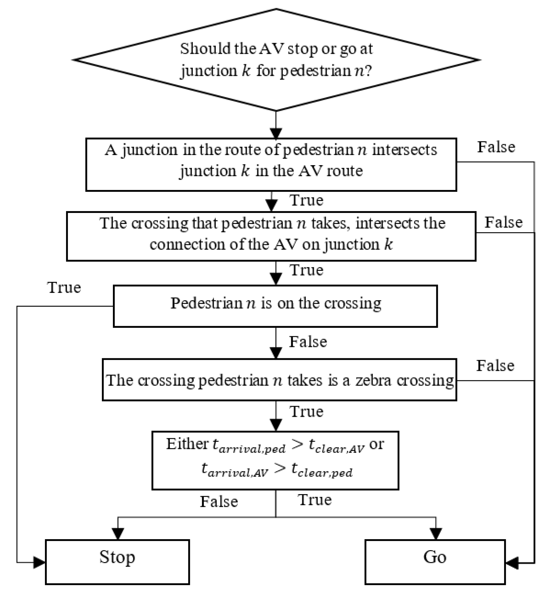
5.1.3. Pedestrian Model

It is assumed that pedestrians can enter only crossroads at dedicated crossings, which are located at junctions. A distinction is made between prioritized and unprioritized crossings. The pedestrian model can be considered part of the junction model, but a distinction is made between the two because of the different calculations and logic. In Figure 4, the decision scheme of the pedestrian model is given.

To prevent congestion on the junction, the allowed braking distance considered by the AV is the distance to the junction, which is not necessarily the distance to the crossing. To calculate accurate arrival and clear times for the pedestrian, Equations (11) and (12) are used. The acceleration and deceleration rates of the pedestrians are very high in comparison to their maximum speed. Therefore, the calculations are simplified for the pedestrians. It is assumed that they can go from a standstill to maximum speed instantly and vice versa. When the decision scheme’s outcome for a crossing on junction k is “stop”, the safe speed is set to the maximum speed for the AV to brake in time for junction k, calculated by Equation (5).

$$t_{arrival,ped}=\frac{g_{crossing,ped}}{v_{max,ped}}=TT{Z}_{ped}$$

(11)

where: $g_{crossing,ped}:$ Gap between crossing and $x$ [m].

$$t_{clear,ped}=\frac{g_{crossing,ped}+w_{crossing}}{v_{max,ped}}$$

(12)

where: $w_{crossing}$: Width of the crossing and $x$ [m].

5.2. Surrogate Safety Indicator Devices

To evaluate the network’s safety, the AVs are outfitted with SSI devices that record the time, position, speed, route and estimate the conflict point location of the vehicles within a straight-line distance of 100 m. The standard SUMO SSI devices calculate DRAC, TTC, and PET only for vehicles and not for pedestrians. Because the time, position, speed, and conflict points are logged, other indicators can be calculated after the simulation has finished. The additional calculated indicators are STCT, TA, TIT, MTTC, CI, PSD, and CrF. When considering the STC, the level of seriousness is estimated by linear interpolation of STCT’s severity level graph. SUMO does not natively support SSI evaluation for pedestrians. Therefore, an SSI device had to be created, which logs the pedestrians’ time, position, and route within the straight-line distance of 100 m. The same indicators are calculated, except for CS, which has been substituted by the PRI.

The only evasive action that can be taken by the AV in this environment is braking. Swerving and accelerating (above the speed limit) is not modeled. Estimating the exact moment of the evasive action is non-trivial in microsimulations (similar to real life). An acceptable threshold for determining whether a braking event is considered an evasive action is a deceleration of more than 2 m∙s⁻² [9]. This will be used to calculate TA, STCT, and other TA-based indicators.

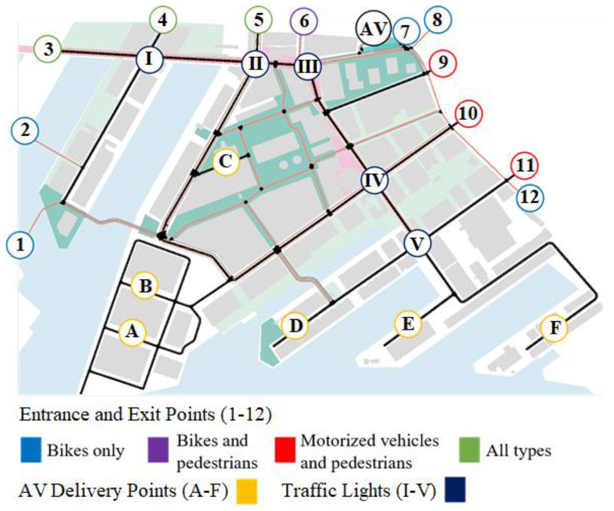
6. Case Study of The Merwe-and Vierhavensgebied

The former Merwe- and Vierhavensgebied (M4H) in the Dutch city of Rotterdam is the use case in this research. It has been a part of the port of Rotterdam, but as the industry grew, most of the port activities were moved to the Maasvlakte area. As this happened, the port and city got separated. This left the municipality with large, partly unused regions close to the city center. To reconnect the port to the city, Rotterdam started the M4H project. The project aims to repurpose the former port area by joining the Makers District [2]. The Makers District consists of several sub-areas, which all have a different mixture of new manufacturing industries, urban facilities, housing, and culture.

The spatial framework provided by the M4H team offers a glance into the future of M4H. The framework provides a map of the M4H in 2035 and a look ahead to 2050. The provided map serves as the basis of our use case. An autonomous vehicle route is suggested in the framework, which is specially designed for autonomous public transport. As autonomous freight transport will undoubtedly play a part in developing new manufacturing industries, the idea is to extend the suggested route to support such autonomous transport. This research investigates what infrastructure, driving behavior, and communication systems are essential for safe and efficient transport. We develop the simulation model using the Python-based open-source simulation framework, SUMO (Simulation of Urban MObility). The network is evaluated as proposed in Figure 5.

The traffic at the entrance and exit points are distributed according to an assumed traffic inflow and outflow ratio, and the weights are presented in

Table 3. Vehicle weights at the entrance and exit points.

Entrance/Exit Points	Cars	Trailers	Bikes	Pedestrians
1	-	-	1	-
2	-	-	1	-
3	1	1	1	1
4	0.5	1	1	1
5	1	1	0.5	1
6	-	-	1	1
7	-	-	2	-
8	-	-	1	-
9	0.5	0.5	-	2
10	1	1	-	2
11	0.5	2	-	1
12	-	-	2	-

. The weights of the delivery points are set to 1.

6.1. Benchmark

Multiple simulation scenarios are investigated to verify the safety and efficiency evaluation methodology and obtain a benchmark for the zone as it is designed now. In these scenarios, the car-following time gap ($\tau$) of the AVs is varied from 1 to 2.5 s, with steps of 0.5, which also affects the AVs’ speed when approaching junctions. For all scenarios, the same random seeds are used to ensure that the same traffic is injected. There are two types of simulation sets. The first set consists of 30 seeds, and each seed runs for 12.000 s (excluding 1.000 s warm-up time). The number of potential accidents, introduced later, is a better measurement for the amount of collected data than the number of seeds and runtime. Since the actual network is rarely fully congested, it is believed that interactions at higher velocities and lower traffic densities are a better representation of the real network behavior. This first set is also used to evaluate the time loss compared to free-flowing vehicles. It is thought that higher delays of the AVs cause other traffic partitions to be more irritated, resulting in a more aggressive driving style [49].

In the second set of simulations, the traffic density is steadily increased until the network is sufficiently gridlocked. The traffic flow, average speed, and density are recorded, and the MFDs are generated for all scenarios. Then, the MFDs are used to confirm that there are no large differences in the network performance due to randomness between runs or any modeling errors. As the fraction of AVs gets small at higher traffic densities, it is believed that the MFDs should converge.

6.1.1. Safety Assessment

Potential accidents are distinguished by calculating STCT, PET, and DRAC_max and subjecting them to the threshold values of

Table 4. SSI threshold values to determine a potential accident.

SSI	Potential Accident Thresholds
STCT	>21
PET	<5
DRACmax	>2

. In

Table 5. The number of potential accidents for the various benchmark scenarios.

Entity Type	τ = 1	τ = 1.5	τ = 2	τ = 2.5
Vehicles and Bikes	60,375	58,636	57,455	57,543
Pedestrians	46,777	47,538	48,545	49,814

, the number of analyzed potential accidents is shown. If one or more thresholds are violated, the incident is marked as a potential accident, and it will be subjected to a full safety assessment by means of SSIs represented in

Table 6. SSI threshold values as used in the safety assessment.

SSI	Vehicles and Bikes	Pedestrians	Comment
STCT	>25	>25	One level safer than original work [42].
TTCmin	<1.25	<1.25	Commonly used [3].
TA	<1.5	<1.5	Commonly used [3].
TIT	>0.35	>0.35	Determined from data.
MTTCmin	<4	<3	Commonly used, slightly tighter for pedestrians [26].
CImax	>10	-	Determined from data.
PET	<3	<3	Slightly tighter [50].
PSDmin	<1	<1	Commonly used [27].
DRACmax	>2.5	>2.5	Maximum braking acceleration, slightly tighter [51].
CrFmax	>50	>50	Determined from data.
PRI	-	>0.1	Determined from data.

.

By using these three indicators, all typical critical safety situations are caught. STCT captures both the AV speed and time of the evasive actions. The PET indicator captures potentially critical conflicts without evasive actions. Finally, DRAC gives insight into the required braking capability. Time, distance, and deceleration are considered by judging all conflicts with these SSIs. This preselection guarantees that SSIs for non-critical conflicts are not calculated. If tighter thresholds are used, STCT, PET, and DRAC_max may report the conflict as non-critical, while other SSIs might consider it critical. Potential accidents that violate the threshold for a certain SSI are reported as an accident for this SSI. Since the total number of incidents differs per scenario due to random chance, the number of accidents for a given SSI is divided by the total number of incidents of each scenario.

The resulting fraction is used to compare the level of safety. The incorporated threshold values are presented in Table 6.

Threshold values for STCT, TTC_min, TA, MTTC_min, PET, PSD_min, and DRAC_max come from the literature, where some adjustments are made to capture more SII accidents. CI_max, CrF_max, and PRI have no thresholds in the literature because they describe the severity of conflicts. However, it is assumed that the safety level can still be judged using thresholds. Thresholds to capture enough SSI accidents are determined by evaluating the obtained data. A similar approach is taken when determining a threshold for the TIT indicator. This way, the four indicators can still be useful for comparing safety among different scenarios.

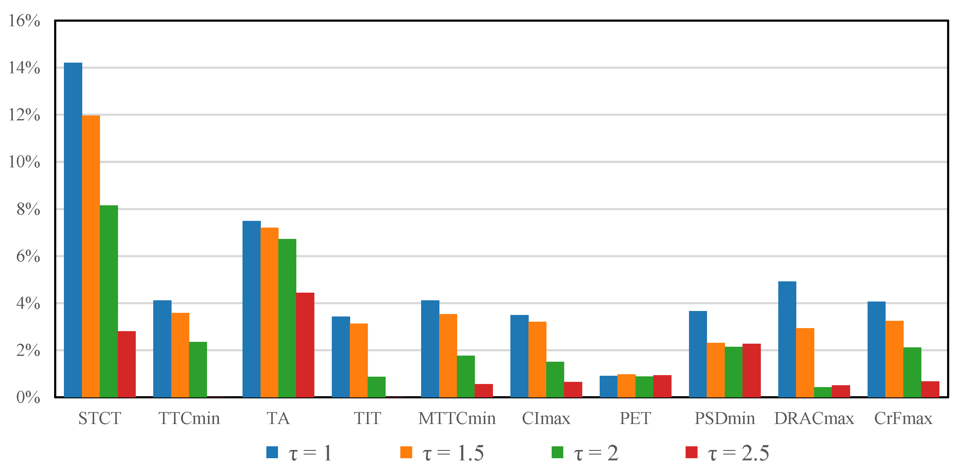
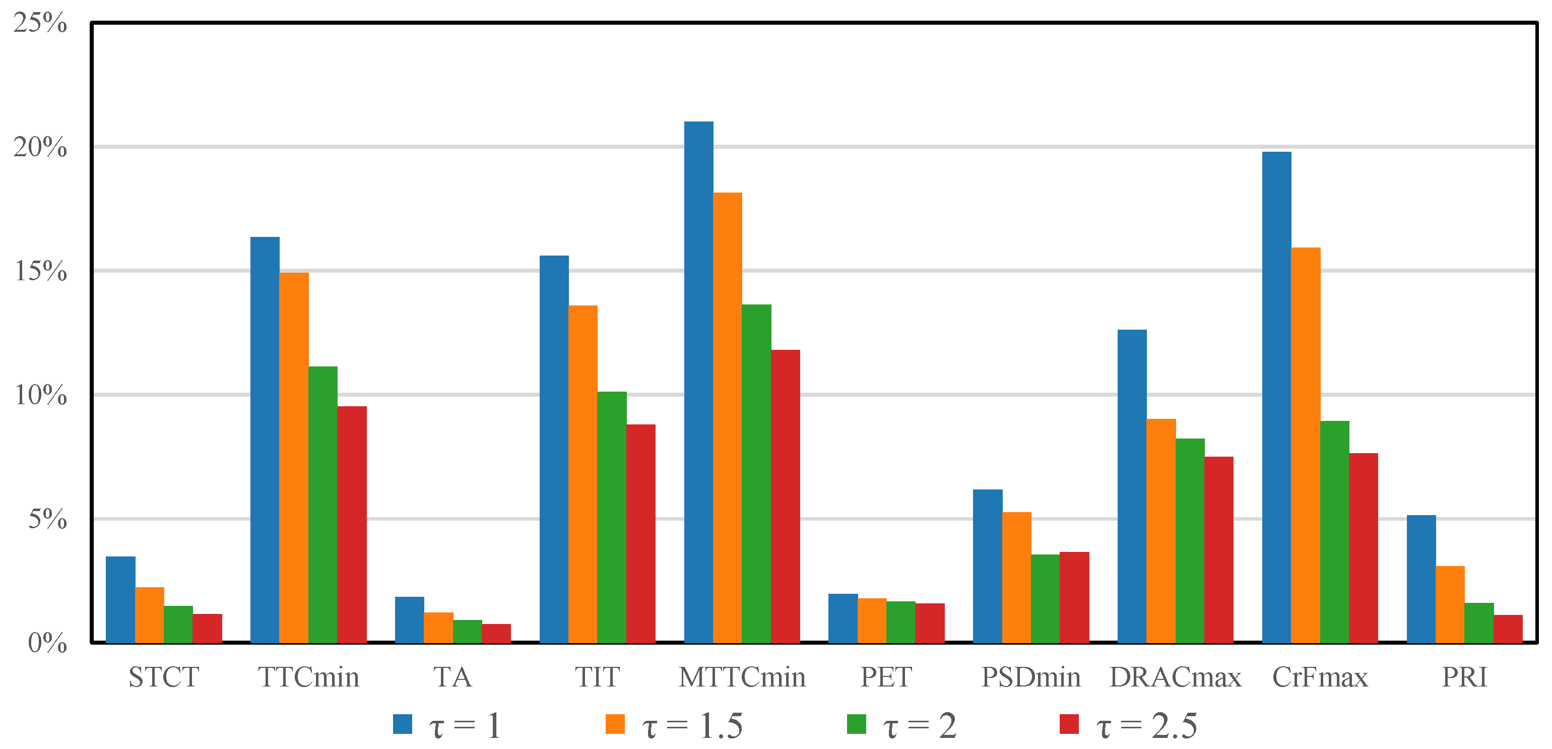
The obtained data on accidents involving AVs, vehicles, and bikes as determined by the SSI assessment are presented graphically in Figure 6. Nearly all indicators show a reduction in the number of accidents as the car-following time gap increases, except the PET and PSD. The results of the SSI assessment involving AVs and pedestrians are presented in Figure 7. All SSIs show a decrease in accident frequency when the car-following time gap of the AVs increases.

6.1.2. Efficiency Evaluation

Aside from the varying car-following time gap scenarios, a scenario without AVs is simulated to investigate if a small ratio of AVs impacts network performance. In order to evaluate the time loss of the vehicles under the scenarios, the free-flow time of all routes is required. This is generated by injecting the appropriate vehicle three times for each route while there are no other vehicles in the system and taking the average time in the system. For the AVs, the time-following gap was set to 2 s when generating the free-flow times. The first set of simulation results is used to calculate the time loss fraction. Due to the random impact of traffic lights, certain entities’ time in the system may be lower than the free-flow time.

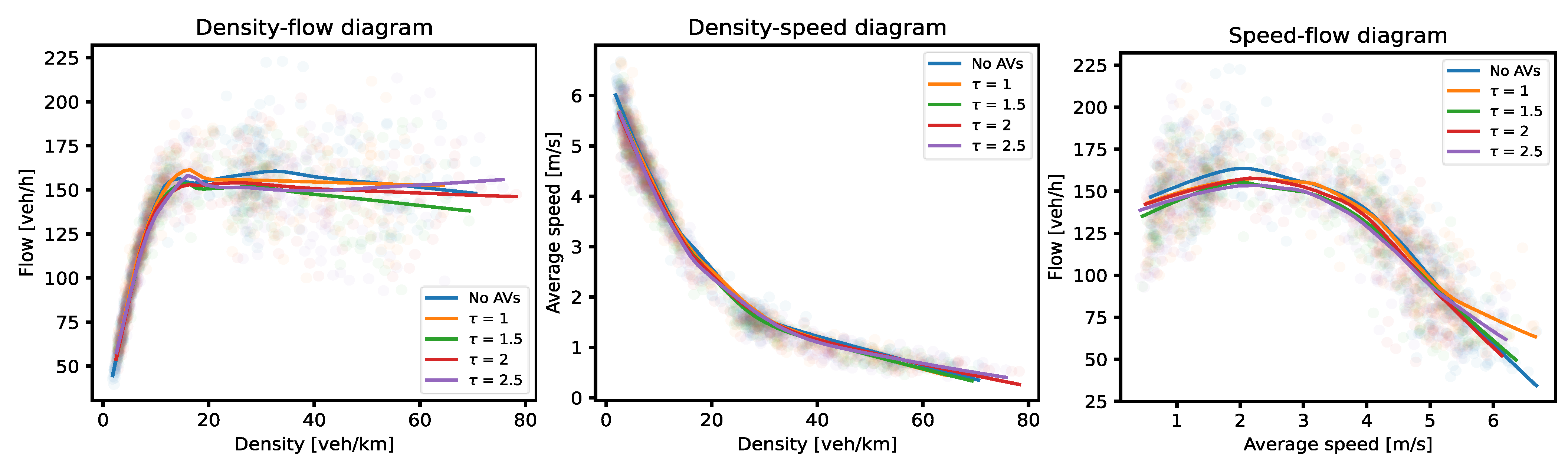
Macroscopic Fundamental Diagrams

Figure 8 shows the MFDs of all scenarios, where a scenario without AVs was also added for comparison. From the density-flow and speed-flow diagrams, it is observed that the scattered flow rates become chaotic at higher vehicle densities and lower average speeds, respectively. Interestingly, the density-speed diagram shows a relation with little scatter for all densities and speed compared to the other diagrams. In general, no significant differences in MFDs are observed. In low scatter regions, the MFDs are almost identical, and in higher scatter parts, the uncertainty gets too high to be meaningful.

Time Loss

The time loss analysis results are presented in

Table 7. The average percentage of delay compared to free-flowing vehicles.

Entity	τ = 1	τ = 1.5	τ = 2	τ = 2.5
AVs	27.4%	29.7%	32.7%	36.6%
Bikes	4.6%	4.6%	4.5%	4.6%
Cars	19.6%	20.0%	19.9%	20.6%
Trailers	18.0%	18.2%	18.2%	18.7%

. The time loss of the AVs gets significantly higher as the car-following time gap increases (

Table 8. Results of independent t-test for delays of car-following time gap 1 and 2.5 s.

Entity	p-Value	H0 Rejected (p < 0.05)
AVs	4.45 × 10−115	29.7%
Bikes	0.865	4.6%
Cars	3.63 × 10−6	20.0%
Trailers	6.05 × 10−2	18.2%

). Bikes do not show a change in delay by the varying car-following parameter. Cars seem to be slightly influenced by the more conservative driving of the AVs, confirmed by the t-test (Table 8). Trailers show an increase in delay caused by the AVs’ car-following parameters, but the H₀ cannot be rejected.

Discussion

It was observed that with increasing car-following time gap, the number and severity of accidents decreased concerning most of the SSIs for AV-AV, AV-trailers, AV-cars, and AV-bikes interactions. The frequency of accidents for the PET and PSD did not or only slightly decrease. This can be caused by the disturbance vehicles instead of the AVs, imperfections in the AVs driving model, or that they are simply not affected by the car-following time gap. The SSI assessment for AV-pedestrian interaction shows promising results. All SSIs decreased with increasing car-following time gap.

The reductions in accidents are probably more profound in the pedestrian assessment since there is only one type of conflict crossing). The PET decreased less than the other SSIs, likely for the same reasons as in the previous paragraph. Although there is a fairly large scatter, the MFDs are considered sufficiently similar to conclude that a small fraction of AVs does not have an unrealistically large effect on the network performance. The MFDs are so similar that the introduction of AVs may not have an impact on the MFD at all.

The results of the time loss analysis show that the time loss of the AVs gets higher as the car-following time gap increases. Cars are slightly influenced by the more conservative driving of the AVs. For trailers, this could not be confirmed, but it is suspected. Longer delays could be dangerous as they could provoke aggressive driving behavior towards AVs, resulting in a less safe driving environment. The bikes did not show any change in delay by varying the car-following parameter. This is because they are mostly separated from other traffic entities in their dedicated lanes.

In short, there exists a trade-off between safety and efficiency when varying the car-following parameters. It is proven that the safety and efficiency analysis methods are sensitive enough to be influenced by driving parameters and possibly by safety measures. In the next subsection, the AV’s desired time gap is set to 2 s, and the safety and operational efficiency results from this section are used for further investigations.

6.2. Main Experiment

From the benchmark, it is known that AVs are prone to critical safety situations and vehicle delays. To improve safety and reduce vehicle delays, five possible measures are investigated, as shown in

Table 9. The different simulation scenarios and their variation on the benchmark.

Scenario	Variation
Benchmark	The OAD model applied to the AVs, with a car-following time gap of 2 s. This is the default AV model on which the other scenarios are based.
V2V	When V2V is enabled and the lidar polygons of two or more AVs intersect (the V2V communication range is the lidar range), the knowledge of all visible disturbance vehicles gets combined, and obsolete pseudo vehicles get removed. Information of other AVs outside the lidar range is not useful as the AV cannot rule out any pseudo vehicles. If the AV is following another AV, a shorter car-following time gap of 1 s is set for the car-following model, and the junction model will be left as it is. Since disturbance vehicles most likely will not have V2V communication systems, only AVs are considered to have V2V available.
V2I	At the busiest and most occluded intersections in the zone, static lidars are placed to observe entities as AVs do. When the polygons of a static lidar(s) and an AV intersect, the information the static lidar has on disturbance vehicles is sent to the AV. Note that the AV does not send its information back to the static lidars, resulting in an undesirable limited type of V2V. With the combined information on disturbance vehicles, obsolete pseudo vehicles can be removed.
V2X	Combines the principles of V2V and V2I.
Slow Down (SD)	Certain non-arterial lanes are subjected to a lower speed limit. By default, all AV/trailer/car lanes have a speed limit of 50 km/h, and the non-arterial are limited to 30 km/h.
Keep Clear (KC)	To reduce unnecessary conservative behavior of the AVs, buildings closer than 10 m to intersections are forbidden. By doing this, the view of the AV should be less obstructed, allowing it to approach junctions at higher (safe) velocities.

. Three measures are communication-based: V2V, V2I, and V2X, while the other two measures are infrastructural-based: reducing the maximum allowed speed and keeping a certain area around intersections clear of obstructions. As the OAD principle should guarantee safe driving behavior in simulated environments, the safety parameters are not expected to change between scenarios. Introducing V2V communication between AVs is relatively cheap as it only requires an extra communication device on the AVs. The additional static sensors in the V2I scenario add a range to the AVs at busy interactions and can collect valuable traffic data, but they are more expensive than V2V. An advantage of V2I is that there are always extra sensors present at a location, while for V2V, it depends on AVs’ presence.

For each measure, a simulation scenario is created. Like the benchmark, two sets of simulation results are used for each scenario. The first set is used to evaluate the SSIs and time loss of the entities. This is done by simulating the network at low traffic densities for 12.000 s (excluding 1000 s warm-up) with 30 different seeds, where the same seeds are used for each scenario. In the second set, the number of disturbance vehicles is steadily increased until the network is sufficiently gridlocked. During these simulations, the traffic flow, density, and average speed are recorded, and the MFDs are created.

6.2.1. Safety Assessment

The incident types assessed are AV-AV, AV-bike, AV-trailer, AV-car, and AV-pedestrian. The combined results for cars, trailers, and bikes are presented first, and then we provide the results for pedestrians. The number of potential accidents for the different scenarios is shown in

Table 10. The number of potential accidents for the various scenarios.

Entity Type	Benchmark	V2I	V2V	V2X	SD	KC
Vehicles and Bikes	57,455	56,155	52,978	57,637	54,539	57,366
Pedestrians	48,545	51,343	54,165	58,156	48,197	47,945

. For each measure, a simulation scenario is created. Like the benchmark, two sets of simulation results are used for each scenario. The first set is used to evaluate the SSIs and time loss of the entities. This is done by simulating the network at low traffic densities for 12,000 s (excluding 1000 s warm-up) with 30 different seeds, where the same seeds are used for each scenario. In the second set, the number of disturbance vehicles is steadily increased until the network is fully congested.

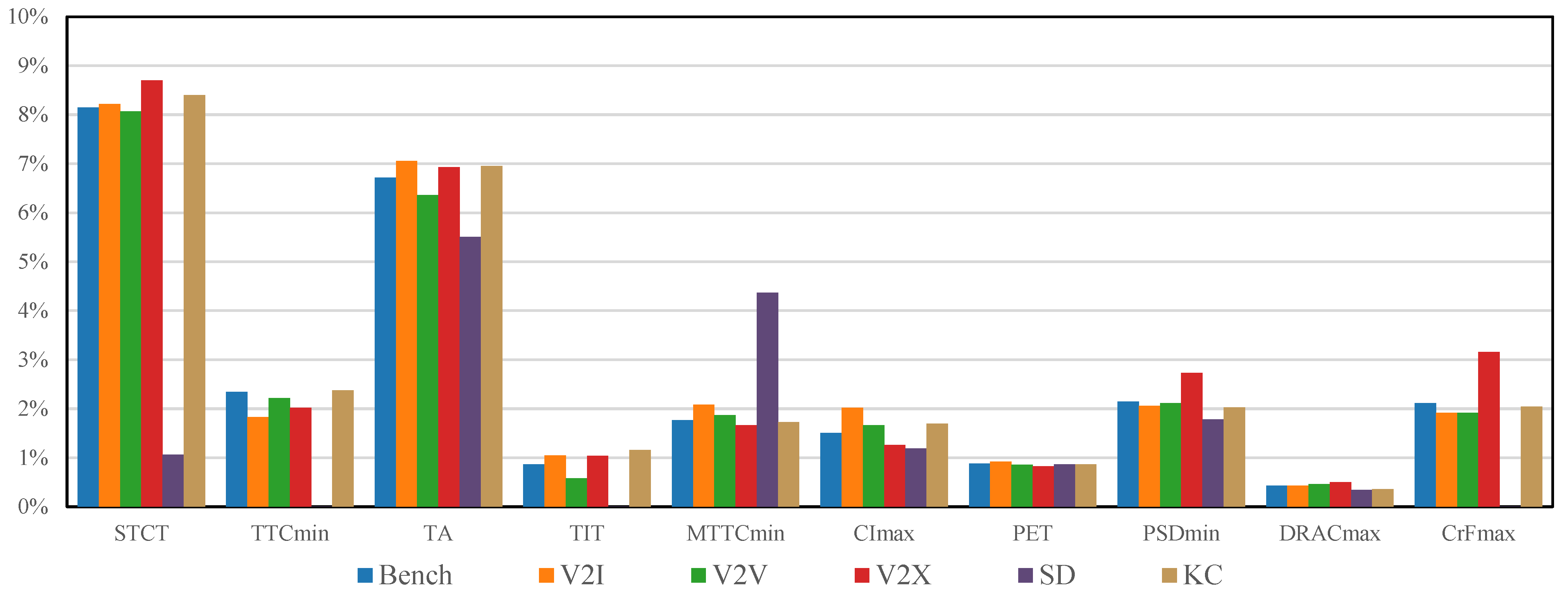
The obtained data regarding accidents involving AVs, vehicles, and bikes as determined by the SSI assessment are presented in Figure 9.

For the V2I, V2V, V2X, and KC scenarios, there is either a slight increase or a slight decrease in accidents according to the SSIs. In the SD scenario, there is a reduction in the recorded number of accidents for all SSIs, except MTTC and PET. MTTC is higher in the SD scenario compared to the benchmark, and PET is about equal.

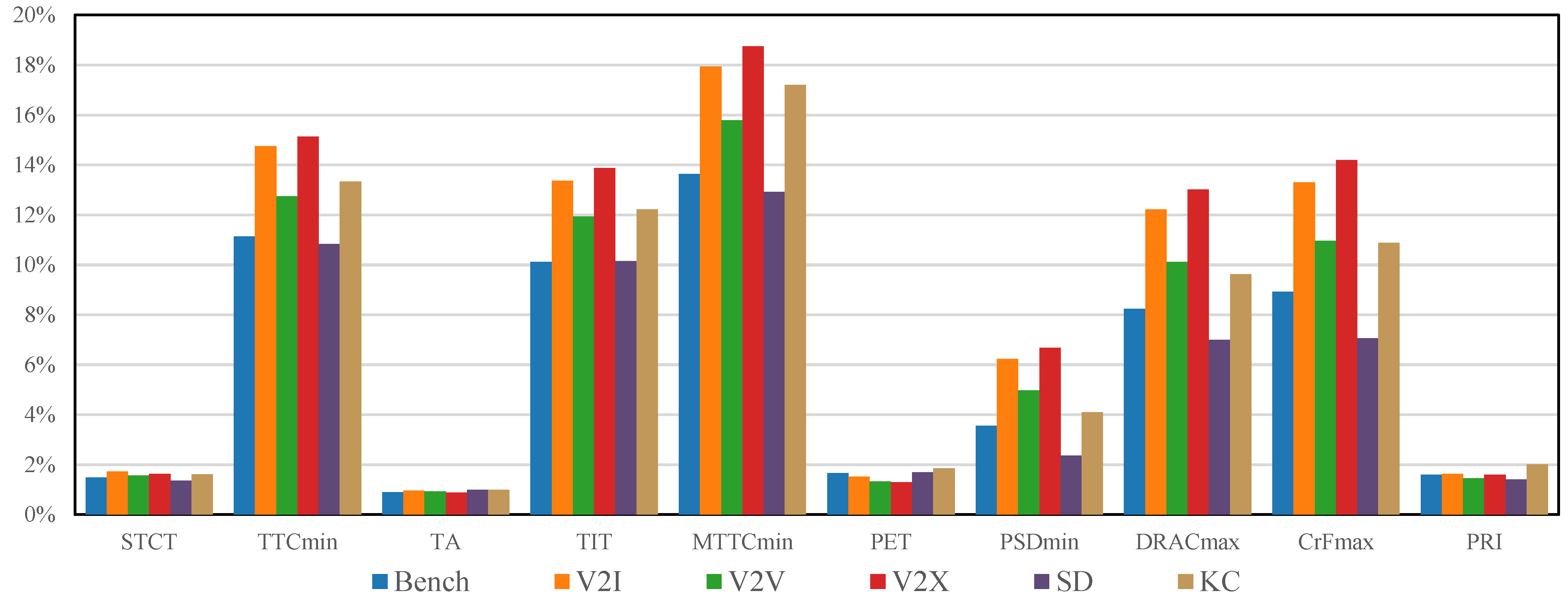
The results of the SSI assessment involving AVs and pedestrians are presented in Figure 10.

All SSIs are relatively equal or higher compared to the benchmark for V2I, V2V, V2X, and KC. Accordingly, one can conclude that applying these measures has not a considerable impact on network safety. This comes as no surprise since the OAD method should guarantee safe driving behavior in simulated environments. For the SD, the reported accidents, according to the SSIs, are about equal or lower than the benchmark.

6.2.2. Efficiency Evaluation

Macroscopic Fundamental Diagrams

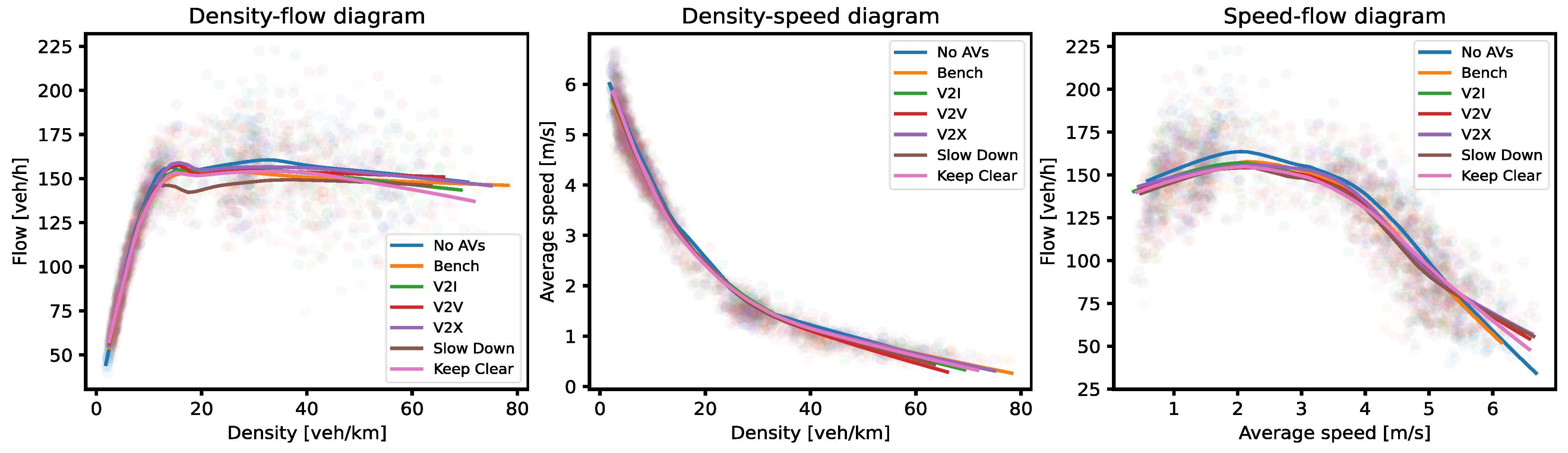
The MFDs for all simulation scenarios are presented in Figure 11. For compassion, a no AV scenario is added again. The scattered flow rate becomes more chaotic at higher vehicle densities and lower average speeds in the density-flow and speed-flow diagram, respectively. The density-speed diagram shows a relation with little scatters across the whole spectrum. When comparing the scenarios in the low scatter regions of the MFD’s, it is clear they perform nearly identical, while in the higher scatter regions of the MFD’s, the similarity in performance between the scenarios is less evident.

Time Loss

Table 11. Performance gain (reduction in average time loss fraction) compared to the benchmark.

Entity	V2I	V2V	V2X	SD	KC
AVs	+7.2%	+6.3%	+7.9%	−14.8%	+3.0%
Bikes	−0.1%	−0.1%	0.0%	−0.2%	−0.1%
Cars	−0.1%	−0.1%	+0.4%	−12.0%	−0.2%
Trailers	+0.1%	−0.3%	−0.1%	−6.2%	−0.1%

shows the performance gain, i.e., reducing time loss, compared to the benchmark scenario. In

Table 12. Results of independent t-test for delays of the benchmark compared to the scenarios.

Scenario		AVs	Bikes	Cars	Trailers
V2I	p-value	6.60 × 10−71	0.215	0.846	0.595
	H0 rejected (p < 0.05)	Yes	No	No	No
V2V	p-value	4.16 × 10−51	0.476	0.555	0.377
	H0 rejected (p < 0.05)	Yes	No	No	No
V2X	p-value	1.73 × 10−78	0.967	0.089	0.962
	H0 rejected (p < 0.05)	Yes	No	No	No
SD	p-value	1.8 × 10−292	2.75 × 10−2	0	4.16 × 10−71
	H0 rejected (p < 0.05)	Yes	Yes	Yes	Yes
KC	p-value	1.29 × 10−14	0.460	0.467	0.883
	H0 rejected (p < 0.05)	Yes	No	No	No

, the results of an independent t-test comparing the time loss fractions of each scenario to the benchmark are presented. It is observed that the AVs experience a statistically significant performance boost (H₀ rejected) in the V2I, V2V, V2X, and KC scenarios. Other entity types do not seem to be significantly affected by these scenarios. All vehicles are significantly affected by the SD scenario, resulting in their worse performance.

6.2.3. Discussion

The results of the safety assessment for AV-AV, AV-trailer, AV-car, and AV-bike interactions showed that for the V2I, V2V, V2X, and KC scenarios, there is either a slight increase or a slight decrease in accidents according to the SSIs. An unexpected finding was the increase in SSI accidents when considering AV-pedestrian interactions (except for the SD scenario), where all SSI accidents were equal or more frequent. This can be explained since there are fewer PVs, or they are further away from intersections and approaching slower compared to the benchmark.

Furthermore, in the SD scenario, it was observed that there are equal or fewer recorded accidents for all SSIs and all entities (except for MTTC in the vehicle SSI assessment). The increase in the number of accidents for MTTC is likely caused by the later braking of AVs. When the AV does not decelerate, the value for MTTC is equal to the TTC. The threshold for MTTC is more than three times higher than TTC, clearly increasing the threshold violations.

When comparing the time loss of the AVs in the benchmark and the V2I, V2V, V2X, and KC scenarios, it becomes clear that there is a considerable performance gain. These performance gains are statistically significant, as confirmed by a t-test at the 0.05 significance level. Keeping a specific area around intersections clear could be a design requirement for new buildings as it improves operational efficiency by 3%. Still, it is probably not economically viable to remove existing objects as the performance gain of adding communication devices is twice as big (6–8%). Interestingly, the V2I and V2V show only a 0.9% difference in performance gain, favoring V2I. When considering the installation and operational costs, only V2V could be regarded as the AVs are already equipped with these sensors and only require an extra communication device. The V2X scenario has achieved the highest performance gain as it combines V2V and V2I. Other entities show no significant performance gain or reduction in the V2I, V2V, V2X, and KC scenarios.

7. Policy Implications

From this research, several policy implications are derived, which can come in handy to make well-informed decisions regarding the deployment of AVs.

• Safe urban living labs for automated driving in mixed-traffic areas can be established, even considering the requirements of VRUs and network efficiency. Introducing a small fraction of AVs will not result in any major changes in network performance or conventional vehicles’ delay at the M4H.
• The operational efficiency of AVs is greatly improved with various means of inter-vehicular communication, while the delay of other vehicles is not majorly affected.
• Keeping a specific area around intersections clear of obstructions also does not impact safety but reduces the delays of AVs.
• Lowering the speed limit is the best way to improve safety, but this may provoke other drivers to speed up. Making the AV’s OAD less effective as it expects other drivers to adhere to the speed limit.

When designing a road network, minimizing the number of interactions between entities from different classes is the best practice from a safety perspective. Dividing traffic with exclusive lanes according to vehicle classes (bike lanes, sidewalks, etc.) is highly advised and is already applied in the M4H network and, in general, in the Netherlands [2]. In the particular case study of the M4H, introducing V2I is highly recommended. Aside from adding extra eyes to the AVs, valuable long-term data can be gathered on the behavior of entities in the zone under different conditions.

Considering the trend towards connected vehicles and infrastructure, it is recommended for the City of Rotterdam to test the V2X technology on these AVs right away. This way, as V2X technology slowly gets available to human-driven vehicles, the necessary developments regarding the AVs are already in full swing.

8. Conclusions

Automated driving research still faces the challenge of establishing safe mixed-traffic operations that consider traffic safety as well as operational efficiency to achieve a sustainable adoption of the technology. Apart from often referenced environmental sustainability aspects, social and economic sustainability aspects involving the interaction between AVs, infrastructure, conventional vehicles, and vulnerable road users such as pedestrians need to be understood and carefully considered in the development process. This work uses the case of an urban area in the Dutch city of Rotterdam to investigate the impact of introducing autonomous vehicles in an urban road network on traffic safety for vulnerable road users and operational network efficiency, and it discusses how to respond this potential impact.

By developing a simulation framework with new junction and pedestrian models as well as virtual AVs with an occlusion-aware driving system, we assess the impact of various measures, including Vehicle-to-Vehicle, Vehicle-to-Infrastructure, Vehicle-to-Everything communications, infrastructure modifications, and driving behavior. We show that traffic safety and network efficiency can be achieved in an urban living lab setting of the considered case.

The results of the benchmark confirm that there exists a trade-off between safety and efficiency when varying the car-following parameters. Additionally, it was proven that safety and efficiency analysis methods are sensitive enough to be influenced by driving parameters. In the main experiment, the Vehicle-to-Vehicle, Vehicle-to-Infrastructure, Vehicle-to-Everything, and Keep Clear scenarios showed similar safety levels for trailers, cars, and bikes, but pedestrian safety slightly decreased. The operational efficiency based on time loss of AVs experienced a performance gain of 7.2%, 6.3%, 7.9%, and 3.0% for these scenarios, respectively. The time loss of the other entities was not affected. Due to the lowered allowed speed in certain lanes, the safety for all entities increased in the Slow Down scenario, at the cost of decreased operational efficiency of all entities. Implementing Vehicle-to-Everything is recommended as it helps the results from the performance perspective. Keeping a certain area around intersections clear is advised for new buildings, and lowering the speed limit is highly suggested as it increases safety. This speed limit is 30 km/h through non-arterial lanes in our experiments. Nonetheless, the impact of emergency vehicles, the weather, lane changing, and overtaking are not investigated. Lane changing and overtaking are preventable in the real network, but emergency vehicles and weather changes are unavoidable. As of now, no distinction was made between conflict location, conflict type, and vehicle types (except pedestrians) when assessing safety. To obtain a better understanding of the crash mechanisms, this distinction will be considered in future work. While this work focuses on pedestrians and cyclists, it would also be interesting to investigate other vulnerable road users and related means of transportation such as scooters, skateboards, segways, or unicycles.