
DEM Study on Hydrological Response in Makkah City, Saudi Arabia


Abstract
1. Introduction
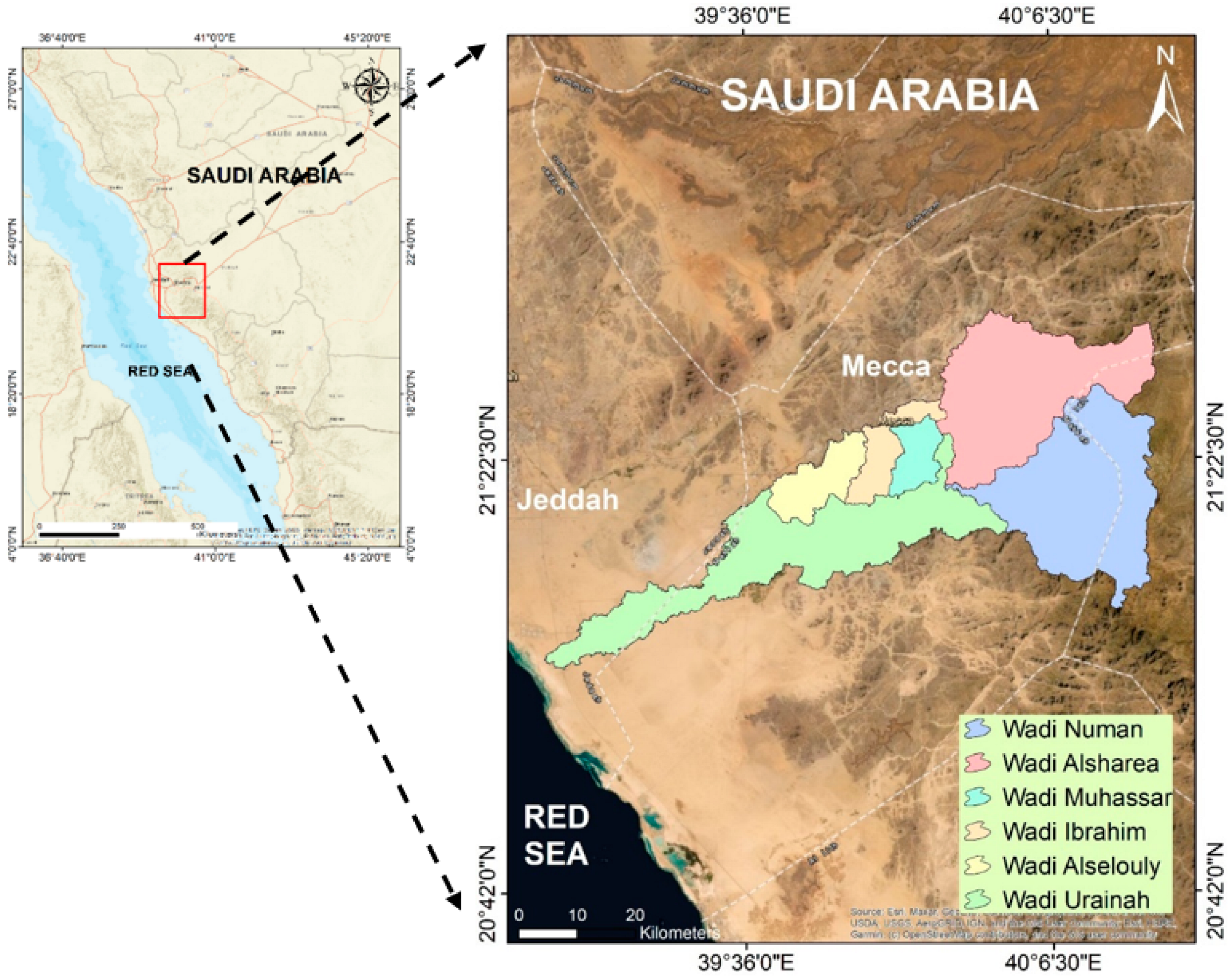
2. Study Area
3. Material and Methodology
3.1. Open Global DEM
- SRTM
- ALOS PALSAR
- Copernicus
3.2. DEM Sentinel-1 Generation
- Perpendicular baseline: The perpendicular baseline (the position of the satellite at the time of acquisition) of the image should have a range of 150–300 m (ESA). The perpendicular baseline is the distance between the satellite’s position at the time of image acquisition. This is different to displacement studies that required a small baseline; DEM generation required a high baseline.
- Temporal baseline: The temporal baseline (different time acquisition) of the image should be as short as possible (6–12 days) to reduce the risk of temporal decorrelation of the phase. The short temporal baseline gives the best result, while the long temporal baseline led to a bad interferogram.
- Atmospheric condition: Some factors in the atmosphere, such as water vapor, can reduce the coherence and quality of the results because they cause phase delays. The recommended condition is good weather and dry conditions with no rainfall.
- Both images must have the same direction: ascending or descending

| Type | Date | Track | Orbit | b_temp (days) | b_perp (m) | Coherence |
|---|---|---|---|---|---|---|
| Master | 02-September-2017 | 14 | 7215 | 0 | 0 | 1 |
| Slave | 14-September-2017 | 14 | 7390 | 12 | 136 | 0.88 |
| Master | 28-August-2018 | 14 | 12,465 | 0 | 0 | 1 |
| Slave | 15-October-2018 | 14 | 13,165 | 48 | 158 | 0.83 |
| Master | 21-September-2018 | 14 | 12,815 | 0 | 0 | 1 |
| Slave | 15-October-2018 | 14 | 13,165 | 24 | 107 | 0.89 |
| Master | 15-October-2018 | 14 | 13,165 | 0 | 0 | 1 |
| Slave | 08-November-2018 | 14 | 13,515 | 24 | 191 | 0.82 |
| Master | 27-October-2018 | 14 | 13,340 | 0 | 0 | 1 |
| Slave | 08-November-2018 | 14 | 13,515 | 12 | 143 | 0.87 |
| Master | 22-September-2020 | 14 | 23,490 | 0 | 0 | 1 |
| Slave | 16-October-2020 | 14 | 23,840 | 24 | 175 | 0.83 |
| Master | 04-October-2020 | 14 | 23,665 | 0 | 0 | 1 |
| Slave | 16-October-2020 | 14 | 23,840 | 12 | 84 | 0.92 |
| Master | 21-November-2020 | 14 | 24,365 | 0 | 0 | 1 |
| Slave | 08-January-2021 | 14 | 25,065 | 48 | 151 | 0.84 |
| Master | 10-December-2021 | 14 | 30,140 | 0 | 0 | 1 |
| Slave | 22-December-2021 | 14 | 29,965 | 12 | 153 | 0.86 |
3.3. GIUH Estimation
- Fill sinks and compute the flow direction and flow accumulations of the DEM using the eight-direction method.
- Obtain stream network by applying a threshold area of 2 km2 of the flow accumulation.
- Delineate the catchment and extract its morphometric parameters using Arc Hydro tools and the morphometric toolbox in GIS.
3.4. Horton Ratios
3.5. Nash Model
- = GIUH parameter
- t = Time (hours)
- = Gamma function
- = Shape and scale parameters proposed by Rosso [39]:
3.6. DEM Validation
4. Results
4.1. DEM of Sentinel-1
4.2. DEM Comparison
5. Discussions
5.1. Limitation of Sentinel-1 DEM
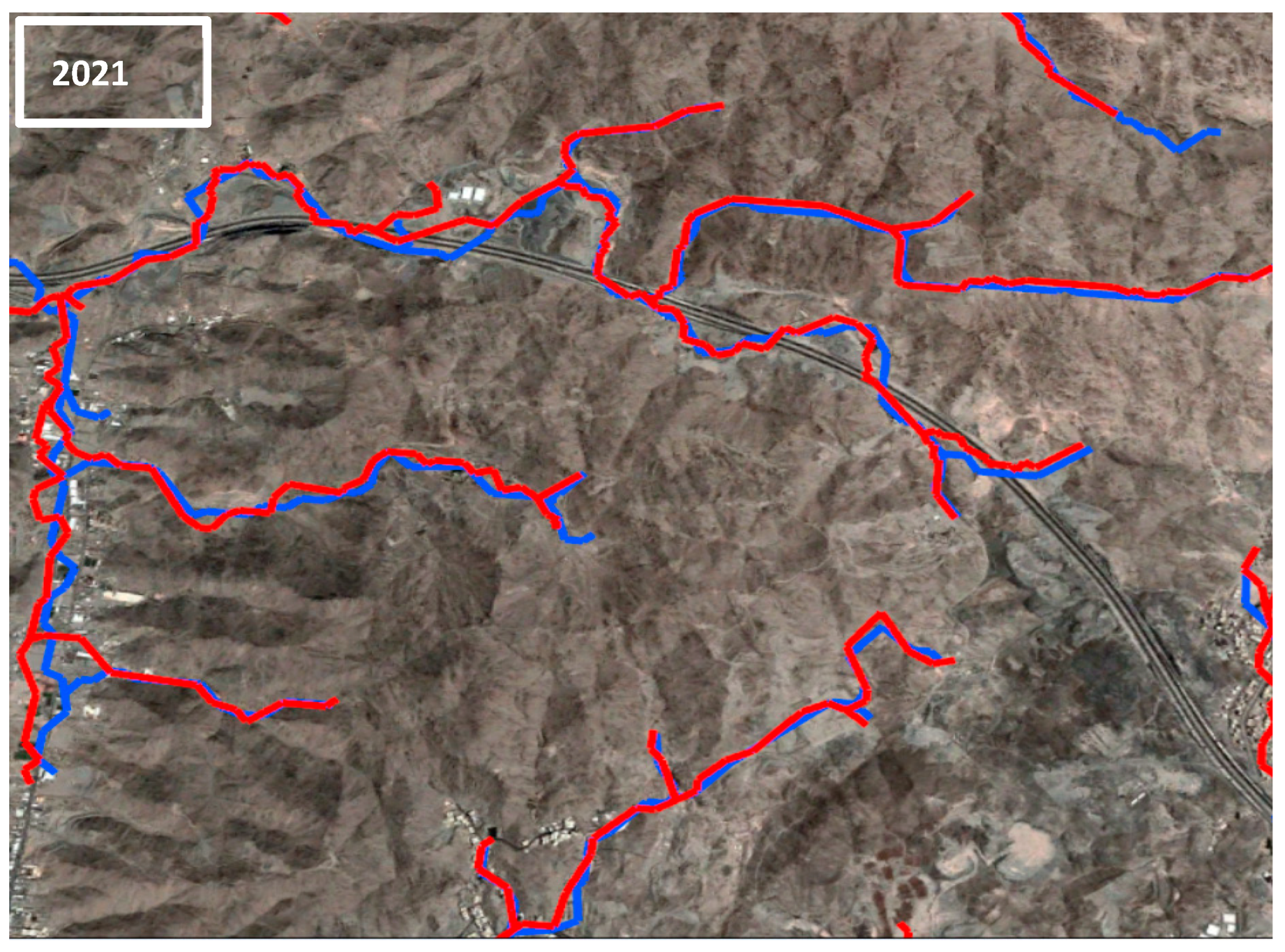
5.2. DEM, GIUH, and Stream Network Comparison
6. Conclusions
- -
- Based on SAR data availability in Makkah City, the best results generated with lower errors compared to other pair images were obtained on 10 December and 22 December 2022. Despite having lower errors, the quality of the Sentinel-1 DEM needs to be improved by using images within a suitable perpendicular baseline, short temporal baseline, and good atmospheric conditions for data acquisition.
- -
- Based on the DEM elevation comparison, Copernicus and SRTM have the highest accuracy, with R2 = 0.9788 and 0.9765 and the lowest RMSE 3.89 m and 4.23 m, respectively. Sentinel-1 and ALOS have the lowest R2 of 0.9028 and 0.9688, and the highest RMSE of 6.31 m and 4.27 m, respectively.
- -
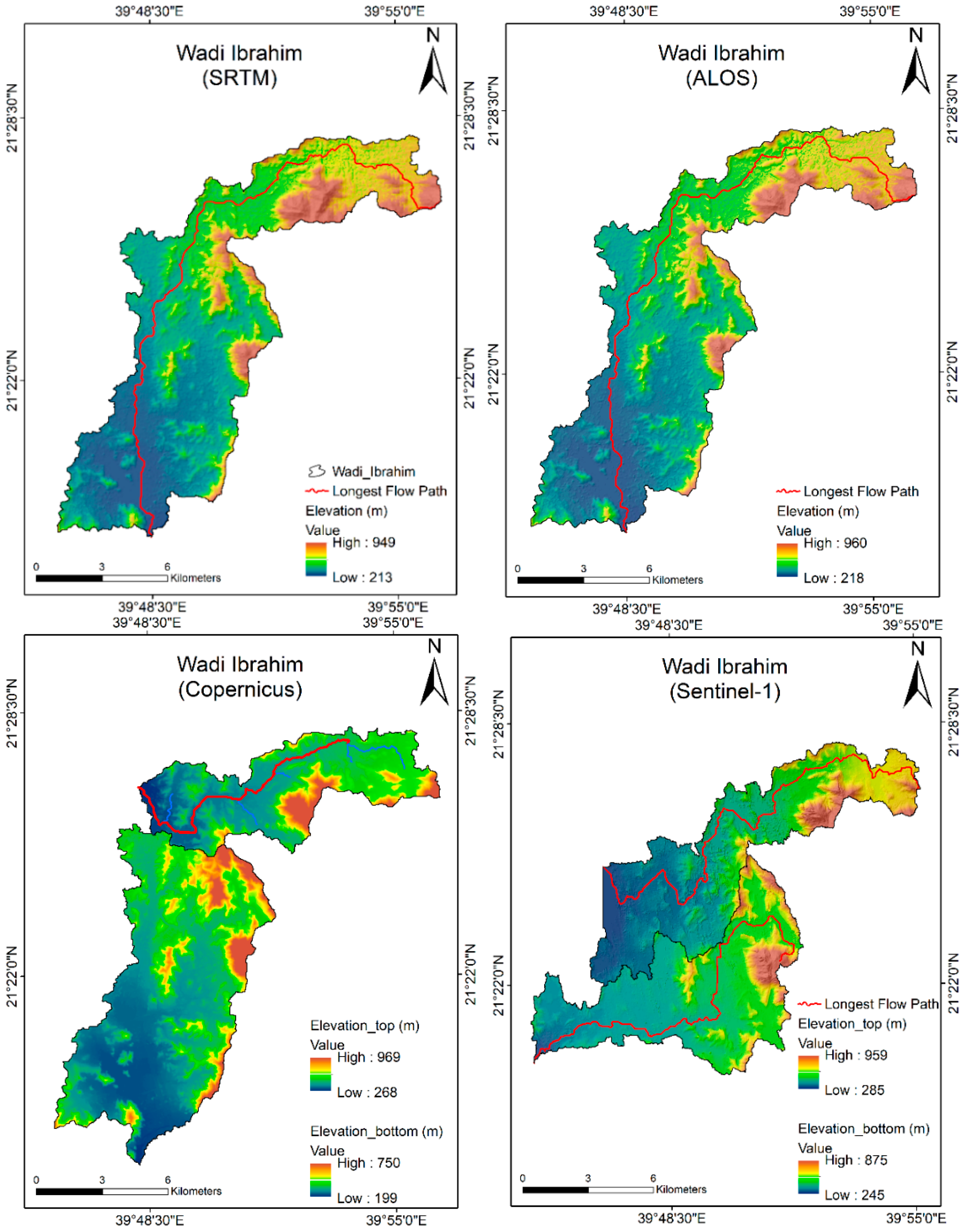
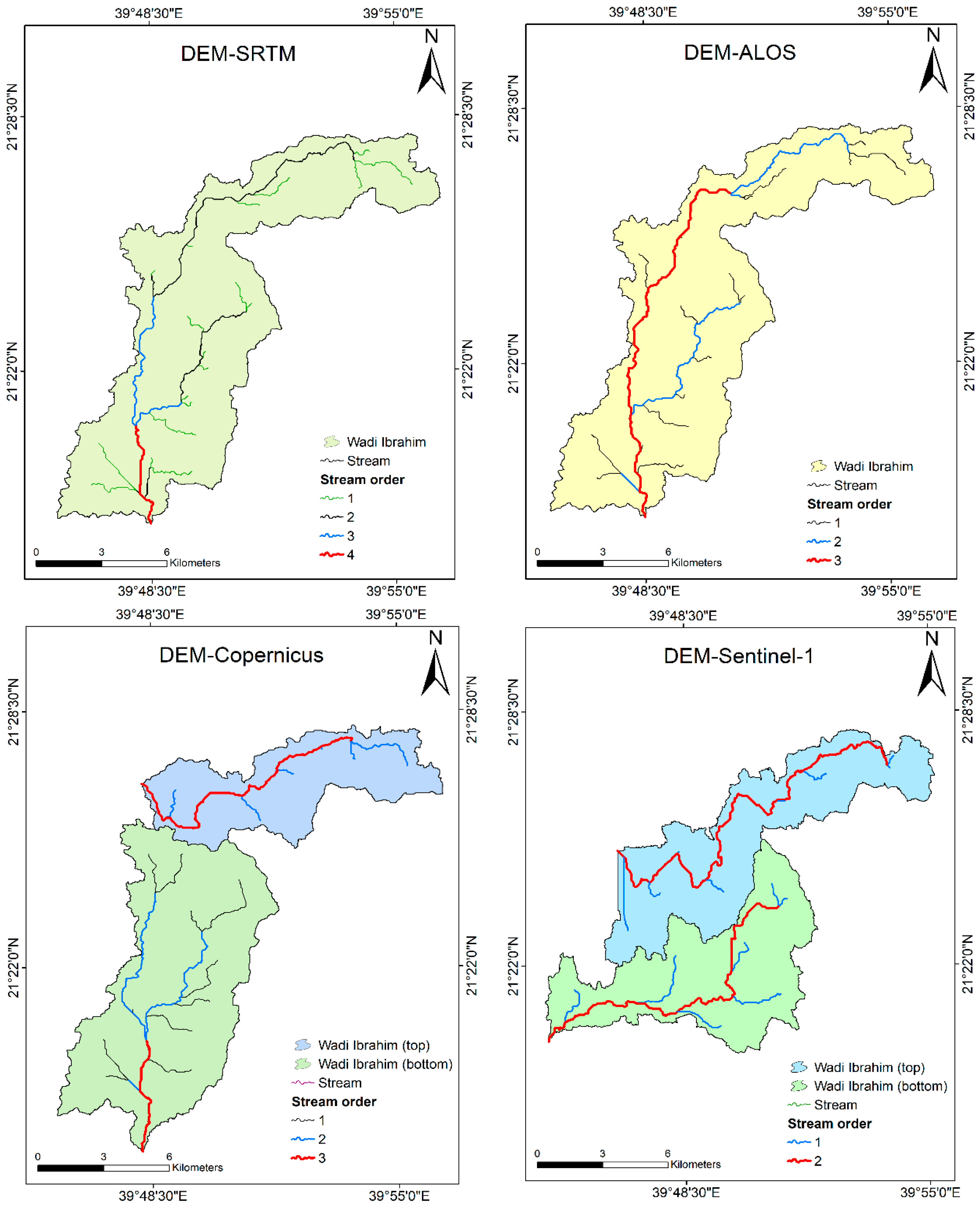
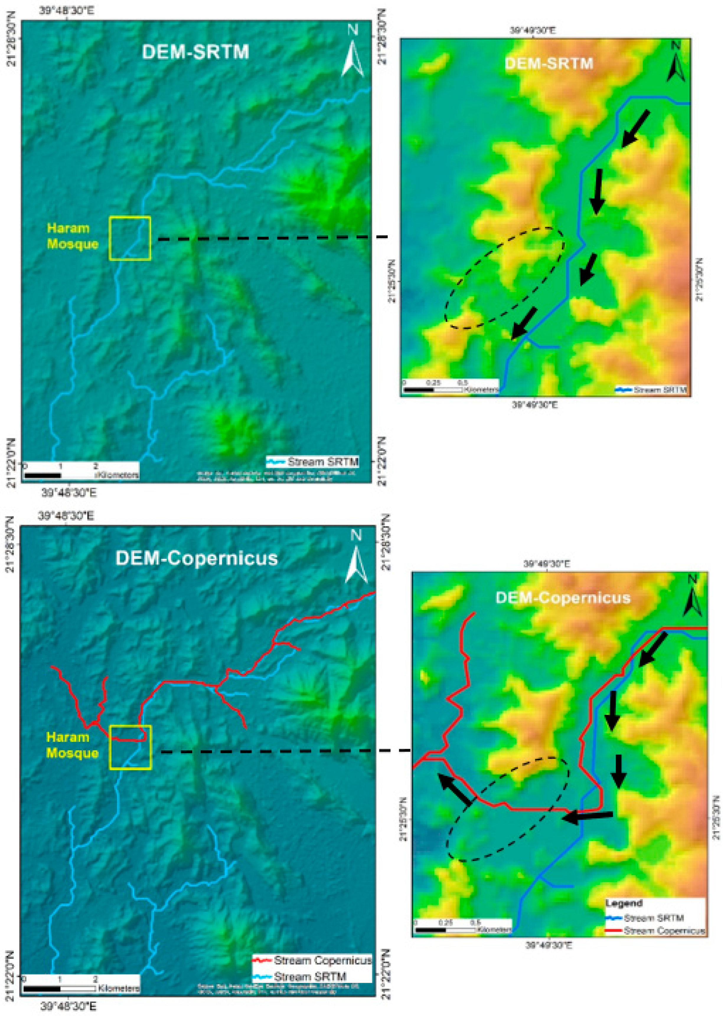
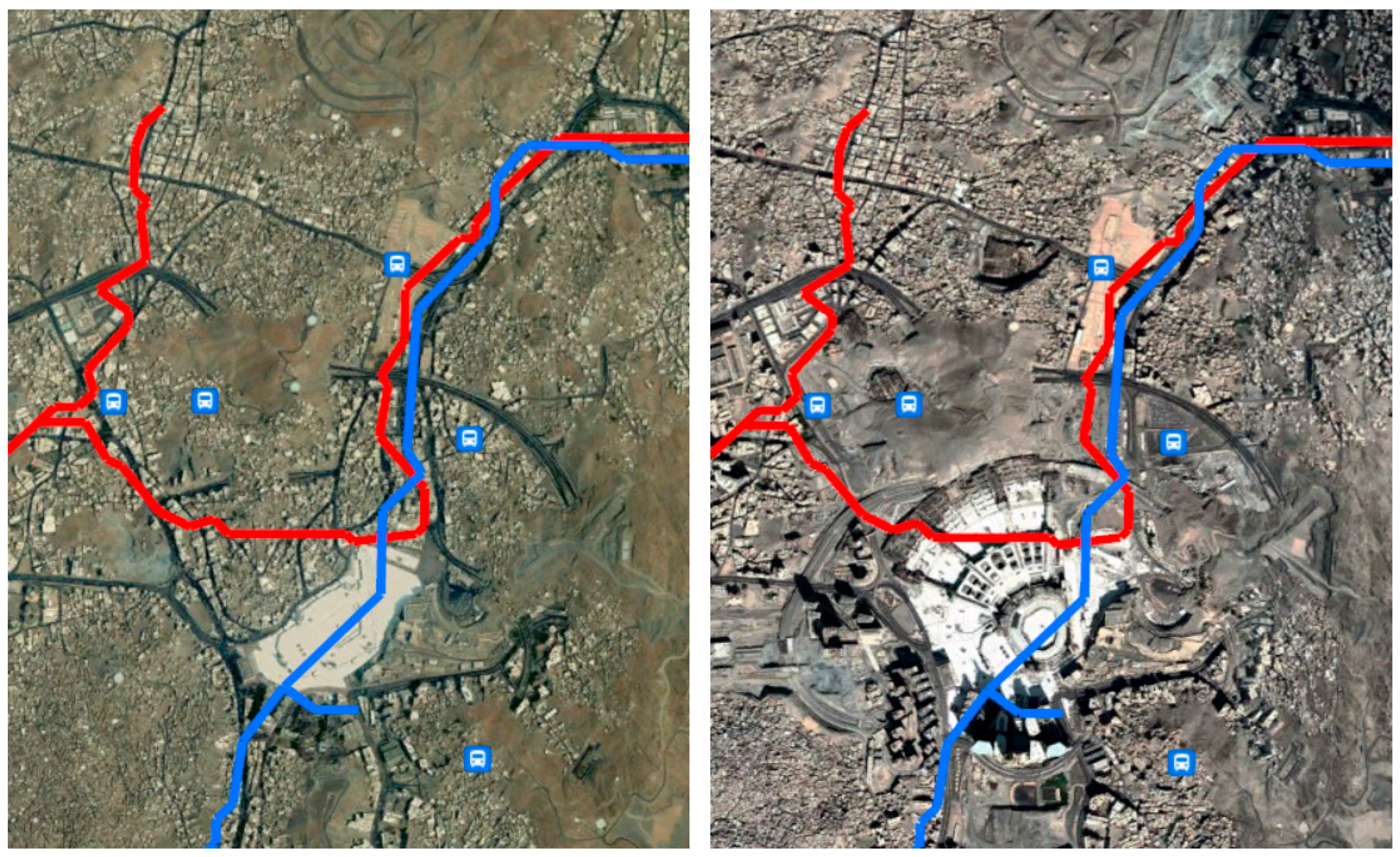
- In Wadi Ibrahim, it was found that the catchment is divided into two sub-wadis based on the Copernicus DEM. This main change in the drainage system in Wadi Ibrahim was due to the continuum of anthropogenic (human) activities around the holy city of Mecca (the mega project of the holy mosque expansion, demolishing mountains, adding buildings, etc.)
- -
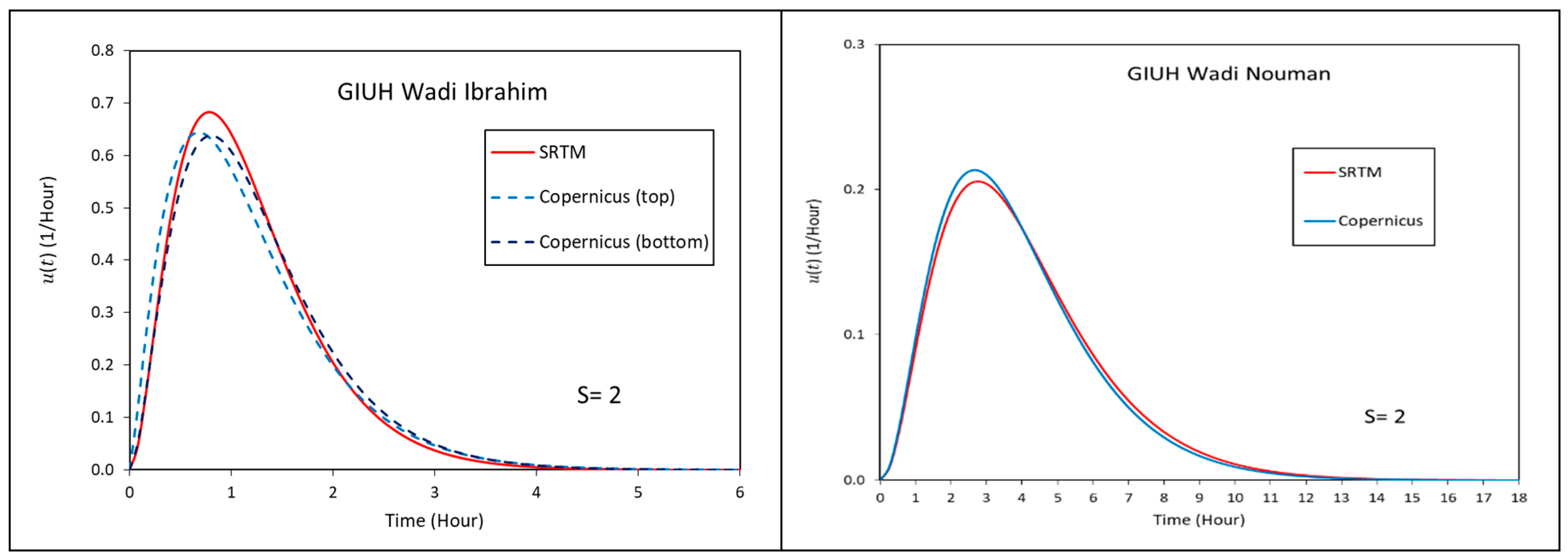
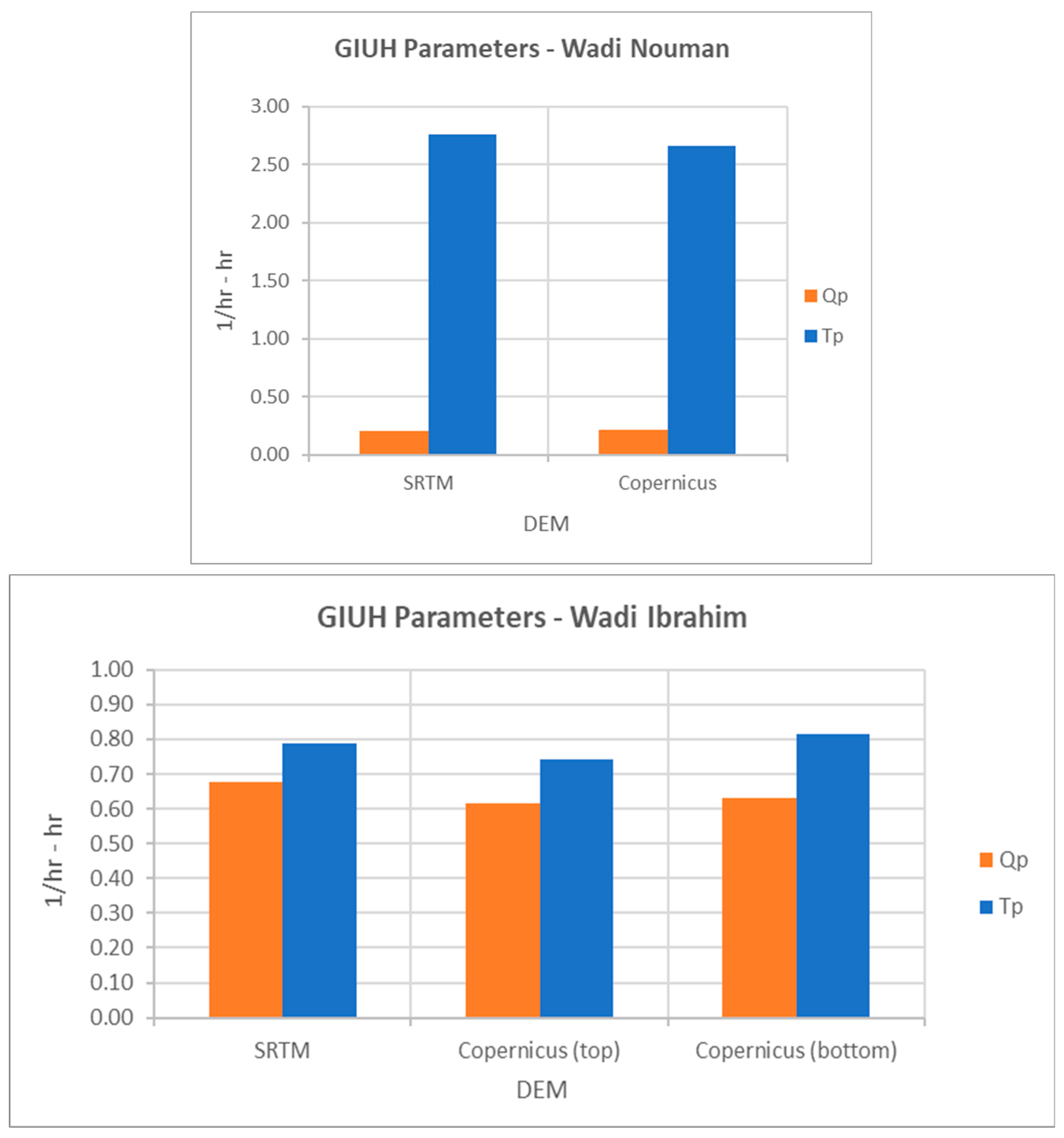
- The stream network and the morphometric parameters (Horton–Strahler ratios) of the catchments vary for both Copernicus and SRTM DEMs and influence the shape of the GIUH.
- -
- The Copernicus DEM for Wadi Nouman has a higher and lower (0.21 and 2.66) than SRTM (0.20 and 2.75). In Wadi Ibrahim, the SRTM has a greater and lower than Copernicus due to the wadi being divided into two sub-wadies.
- -
- The stream network in the mountainous area is quite similar for SRTM and Copernicus due to the dominant influence of the mountainous relief and relatively inconsequential influence of anthropogenic activities and DSM noise. In the urban area, the variation of the stream network is high due to differing DSM noise and significant anthropogenic activities such as urban redevelopment.
- -
- Overall, the Copernicus DEM features the most reliable data quality compared to other open-source data and represents the most recent data.
Author Contributions
Funding
Data Availability Statement
Conflicts of Interest
References
- Chandesris, A.; Van Looy, K.; Diamond, J.S.; Souchon, Y. Small dams alter thermal regimes of downstream water. Hydrol. Earth Syst. Sci. 2019, 23, 4509–4525. [Google Scholar] [CrossRef]
- Elhag, M.; Galal, H.K.; Alsubaie, H. Understanding of morphometric features for adequate water resource management in arid environments. Geosci. Instrum. Methods Data Syst. 2017, 6, 293–300. [Google Scholar] [CrossRef]
- Wang, W.; Shao, Q.; Yang, T.; Peng, S.; Xing, W.; Sun, F.; Luo, Y. Quantitative assessment of the impact of climate variability and human activities on runoff changes: A case study in four catchments of the Haihe River basin, China. Hydrol. Process. 2013, 27, 1158–1174. [Google Scholar] [CrossRef]
- Tang, X.; Fu, G.; Zhang, S.; Gao, C.; Wang, G.; Bao, Z.; Jin, J. Attribution of climate change and human activities to streamflow variations with a posterior distribution of hydrological simulations. Hydrol. Earth Syst. Sci. Discuss. 2021, 2021, 1–37. [Google Scholar] [CrossRef]
- Güler, C.; Kurt, M.A.; Alpaslan, M.; Akbulut, C. Assessment of the impact of anthropogenic activities on the groundwater hydrology and chemistry in Tarsus coastal plain (Mersin, SE Turkey) using fuzzy clustering, multivariate statistics and GIS techniques. J. Hydrol. 2012, 414, 435–451. [Google Scholar] [CrossRef]
- Sadeghi, S.H.; Hazbavi, Z.; Gholamalifard, M. Interactive impacts of climatic, hydrologic and anthropogenic activities on watershed health. Sci. Total Environ. 2019, 648, 880–893. [Google Scholar] [CrossRef] [PubMed]
- Bao, Z.; Zhang, J.; Wang, G.; Fu, G.; He, R.; Yan, X.; Jin, J.; Liu, Y.; Zhang, A. Attribution for decreasing streamflow of the Haihe River basin, northern China: Climate variability or human activities? J. Hydrol. 2012, 460, 117–129. [Google Scholar] [CrossRef]
- Kong, D.; Miao, C.; Wu, J.; Duan, Q. Impact assessment of climate change and human activities on net runoff in the Yellow River Basin from 1951 to 2012. Ecol. Eng. 2016, 91, 566–573. [Google Scholar] [CrossRef]
- Han, Z.; Long, D.; Fang, Y.; Hou, A.; Hong, Y. Impacts of climate change and human activities on the flow regime of the dammed Lancang River in Southwest China. J. Hydrol. 2019, 570, 96–105. [Google Scholar] [CrossRef]
- Xie, J.; Xu, Y.-P.; Wang, Y.; Gu, H.; Wang, F.; Pan, S. Influences of climatic variability and human activities on terrestrial water storage variations across the Yellow River basin in the recent decade. J. Hydrol. 2019, 579, 124218. [Google Scholar] [CrossRef]
- Kumar, A.U.; Jayakumar, K. Hydrological alterations due to anthropogenic activities in Krishna River Basin, India. Ecol. Indic. 2020, 108, 105663. [Google Scholar] [CrossRef]
- Yang, N.; Zhang, Y.; Duan, K. Effect of hydrologic alteration on the community succession of macrophytes at Xiangyang Site, Hanjiang River, China. Scientifica 2017, 2017, 4083696. [Google Scholar] [CrossRef] [PubMed]
- Zhang, Y.; Arthington, A.; Bunn, S.; Mackay, S.; Xia, J.; Kennard, M. Classification of flow regimes for environmental flow assessment in regulated rivers: The Huai River Basin, China. River Res. Appl. 2012, 28, 989–1005. [Google Scholar] [CrossRef]
- Jing, C.; Shortridge, A.; Lin, S.; Wu, J. Comparison and validation of SRTM and ASTER GDEM for a subtropical landscape in Southeastern China. Int. J. Digit. Earth 2014, 7, 969–992. [Google Scholar] [CrossRef]
- Jenson, S.K.; Domingue, J.O. Extracting topographic structure from digital elevation data for geographic information system analysis. Photogramm. Eng. Remote Sens. 1988, 54, 1593–1600. [Google Scholar]
- Farran, M.M.; Elfeki, A.; Elhag, M.; Chaabani, A. A comparative study of the estimation methods for NRCS curve number of natural arid basins and the impact on flash flood predications. Arab. J. Geosci. 2021, 14, 1–23. [Google Scholar] [CrossRef]
- Tarboton, D.G. A new method for the determination of flow directions and upslope areas in grid digital elevation models. Water Resour. Res. 1997, 33, 309–319. [Google Scholar] [CrossRef]
- Elhag, M.; Yilmaz, N. Insights of remote sensing data to surmount rainfall/runoff data limitations of the downstream catchment of Pineios River, Greece. Environ. Earth Sci. 2021, 80, 1–13. [Google Scholar] [CrossRef]
- Erskine, R.H.; Green, T.R.; Ramirez, J.A.; MacDonald, L.H. Comparison of grid-based algorithms for computing upslope contributing area. Water Resour. Res. 2006, 42, W09416. [Google Scholar] [CrossRef]
- Boreggio, M.; Bernard, M.; Gregoretti, C. Evaluating the differences of gridding techniques for Digital Elevation Models generation and their influence on the modeling of stony debris flows routing: A case study from Rovina di Cancia basin (North-eastern Italian Alps). Front. Earth Sci. 2018, 6, 89. [Google Scholar] [CrossRef]
- Hawker, L.; Bates, P.; Neal, J.; Rougier, J. Perspectives on digital elevation model (DEM) simulation for flood modeling in the absence of a high-accuracy open access global DEM. Front. Earth Sci. 2018, 6, 233. [Google Scholar] [CrossRef]
- Saksena, S.; Merwade, V. Incorporating the effect of DEM resolution and accuracy for improved flood inundation mapping. J. Hydrol. 2015, 530, 180–194. [Google Scholar] [CrossRef]
- Purinton, B.; Bookhagen, B. Beyond Vertical Point Accuracy: Assessing Inter-pixel Consistency in 30 m Global DEMs for the Arid Central Andes. Front. Earth Sci. 2021, 9, 758606. [Google Scholar] [CrossRef]
- Karlson, M.; Bastviken, D.; Reese, H. Error Characteristics of Pan-Arctic Digital Elevation Models and Elevation Derivatives in Northern Sweden. Remote Sens. 2021, 13, 4653. [Google Scholar] [CrossRef]
- Karki, S.; Acharya, S.; Gautam, A. Evaluation of the Vertical Accuracy of Open Access Digital Elevation Models across Different Physiographic Regions and 2 River Basins of Nepal 3. 2021. Available online: https://www.researchgate.net/profile/Saroj-Karki-5/publication/351927834_Evaluation_of_the_Vertical_Accuracy_of_Open_Access_Digital_Elevation_Models_across_Different_Physiographic_Regions_and_River_Basins_of_Nepal/links/60b51a2092851cde8846dad9/Evaluation-of-the-Vertical-Accuracy-of-Open-Access-Digital-Elevation-Models-across-Different-Physiographic-Regions-and-River-Basins-of-Nepal.pdf (accessed on 17 July 2022).
- Masoud, M.H.; Basahi, J.; Niyazi, B. Assessment and modeling of runoff in ungauged basins based on paleo-flood and GIS techniques (case study of Wadi Al Dawasir-Saudi Arabia). Arab. J. Geosci. 2019, 12, 483. [Google Scholar] [CrossRef]
- Bahrawi, J.; Alqarawy, A.; Chabaani, A.; Elfeki, A.; Elhag, M. Spatiotemporal analysis of the annual rainfall in the Kingdom of Saudi Arabia: Predictions to 2030 with different confidence levels. Theor. Appl. Climatol. 2021, 146, 1479–1499. [Google Scholar] [CrossRef]
- Rodríguez-Iturbe, I.; Valdés, J.B. The geomorphologic structure of hydrologic response. Water Resour. Res. 1979, 15, 1409–1420. [Google Scholar] [CrossRef]
- Moussa, R. Definition of new equivalent indices of Horton-Strahler ratios for the derivation of the Geomorphological Instantaneous Unit Hydrograph. Water Resour. Res. 2009, 45, W09406. [Google Scholar] [CrossRef]
- Shaaban, F.; Othman, A.; Habeebullah, T.M.; El-Saoud, W.A. An integrated GPR and geoinformatics approach for assessing potential risks of flash floods on high-voltage towers, Makkah, Saudi Arabia. Environ. Earth Sci. 2021, 80, 199. [Google Scholar] [CrossRef]
- Elhag, M.; Alshamsi, D. Integration of remote sensing and geographic information systems for geological fault detection on the island of Crete, Greece. Geosci. Instrum. Methods Data Syst. 2019, 8, 45–54. [Google Scholar] [CrossRef]
- El Bastawesy, M.; Al Harbi, K.; Habeebullah, T. The hydrology of Wadi Ibrahim Catchment in Makkah City, the Kingdom of Saudi Arabia: The interplay of urban development and flash flood hazards. Life Sci. J. 2012, 9, 580–589. [Google Scholar]
- Yousef, B. The climate of Mecca area. J. Umm Al-Qura Soc. Sci. 1992, 15, 1–94. [Google Scholar]
- Braun, A. Retrieval of digital elevation models from Sentinel-1 radar data–open applications, techniques, and limitations. Open Geosci. 2021, 13, 532–569. [Google Scholar] [CrossRef]
- Sahoo, R.; Jain, V. Sensitivity of drainage morphometry based hydrological response (GIUH) of a river basin to the spatial resolution of DEM data. Comput. Geosci. 2018, 111, 78–86. [Google Scholar] [CrossRef]
- Bamufleh, S.; Al-Wagdany, A.; Elfeki, A.; Chaabani, A. Developing a geomorphological instantaneous unit hydrograph (GIUH) using equivalent Horton-Strahler ratios for flash flood predictions in arid regions. Geomat. Nat. Hazards Risk 2020, 11, 1697–1723. [Google Scholar] [CrossRef]
- Horton, R.E. Erosional development of streams and their drainage basins; hydrophysical approach to quantitative morphology. Geol. Soc. Am. Bull. 1945, 56, 275–370. [Google Scholar] [CrossRef]
- Nash, J.E.; HRS. A unit hydrograph study, with particular reference to British catchments. Proc. Inst. Civ. Eng. 1960, 17, 249–282. [Google Scholar] [CrossRef]
- Rosso, R. Nash model relation to Horton order ratios. Water Resour. Res. 1984, 20, 914–920. [Google Scholar] [CrossRef]
- Stilla, U.; Soergel, U.; Thoennessen, U. Potential and limits of InSAR data for building reconstruction in built-up areas. ISPRS J. Photogramm. Remote Sens. 2003, 58, 113–123. [Google Scholar] [CrossRef]
- Castellazzi, P.; Arroyo-Domínguez, N.; Martel, R.; Calderhead, A.I.; Normand, J.C.; Gárfias, J.; Rivera, A. Land subsidence in major cities of Central Mexico: Interpreting InSAR-derived land subsidence mapping with hydrogeological data. Int. J. Appl. Earth Obs. Geoinf. 2016, 47, 102–111. [Google Scholar] [CrossRef]
- Hanssen, R.F. Radar Interferometry: Data Interpretation and Error Analysis; Springer: Berlin/Heidelberg, Germany, 2001; Volume 2. [Google Scholar]
- Elhag, M.; Bahrawi, J.; Aljahdali, M.H.; Eleftheriou, G.; Labban, A.H.; Alqarawy, A. Vertical displacement assessment in temporal analysis of the transboundary islands of Tiran and Sanafir, Egypt-Saudi Arabia. Arab. J. Geosci. 2022, 15, 1–13. [Google Scholar] [CrossRef]
- del Rosario Gonzalez-Moradas, M.; Viveen, W. Evaluation of ASTER GDEM2, SRTMv3. 0, ALOS AW3D30 and TanDEM-X DEMs for the Peruvian Andes against highly accurate GNSS ground control points and geomorphological-hydrological metrics. Remote Sens. Environ. 2020, 237, 111509. [Google Scholar] [CrossRef]
- Elhag, M.; Hidayatulloh, A.; Bahrawi, J.; Chaabani, A.; Budiman, J. Using inconsistencies of wadi morphometric parameters to understand patterns of soil erosion. Arab. J. Geosci. 2022, 15, 1–14. [Google Scholar] [CrossRef]
- Bahrawi, J.; Ewea, H.; Kamis, A.; Elhag, M. Potential flood risk due to urbanization expansion in arid environments, Saudi Arabia. Nat. Hazards 2020, 104, 795–809. [Google Scholar] [CrossRef]
- Marešová, J.; Gdulová, K.; Pracná, P.; Moravec, D.; Gábor, L.; Prošek, J.; Barták, V.; Moudrý, V. Applicability of Data Acquisition Characteristics to the Identification of Local Artefacts in Global Digital Elevation Models: Comparison of the Copernicus and TanDEM-X DEMs. Remote Sens. 2021, 13, 3931. [Google Scholar] [CrossRef]
- Mutar, A.Q.; Mustafa, M.T.; Hameed, M.A. The impact of (DEM) Accuracy on the Watersheds areas as a function of spatial data. Period. Eng. Nat. Sci. 2021, 9, 1118–1130. [Google Scholar] [CrossRef]


| DEM | Parameter | ||||
|---|---|---|---|---|---|
| Resolution | Sources | Acquisition Year | Released Year | Band | |
| SRTM | 30 m | NASA | 2000 | 2013 | C |
| ALOS | 12.5 m | JAXA | 2009 | 2014 | L |
| Copernicus | 30 m | ESA | 2011–2014 | 2021 | X |
| Sentinel-1 | 13.5 m | ESA | 2015–Now | 2015 | C |
| Steps | Descriptions |
|---|---|
| Read data | Read data from two different SAR images |
| TOPSAR Split | Select the area of interest (IW2 and IW3, bursts 2–5, VV Polarization) |
| Apply Orbit File | Correct satellite and orbit geometry |
| Back Geocoding | Make over stack between two images |
| Interferogram | Generate phase and coherence |
| TOPSAR deburst | Remove the seamline/space between the bursts |
| TOPSAR merge | Merge the subswath IW2 and IW3 |
| Goldstein Phase Filtering | Reduce the phase noise |
| Multilooking | Reduce the inherent speckle noise |
| Snaphu unwrapping | Export, unwrapping, and import of phase |
| Phase to Elevation | Convert phase to elevation (DEM) |
| Terrain Correction | Geometric correction to project the map into WGS84 |
| Basin Parameters | Wadi Nouman | |||
|---|---|---|---|---|
| SRTM | ALOS | Copernicus | Sentinel-1 | |
| Low Elevation (m) | 282 | 284 | 263 | 504 |
| High Elevation (m) | 2605 | 2611 | 2611 | 2787 |
| Area (km) | 678.6 | 695.7 | 694.9 | 747.7 |
| Perimeter (km) | 210.7 | 212.6 | 217.9 | 229.3 |
| Longest flow path (km) | 68.7 | 68.5 | 67.2 | 68.3 |
| Basin Length (km) | 47.4 | 47.2 | 49.3 | 41.2 |
| Basin Parameters | Wadi Ibrahim | |||||
|---|---|---|---|---|---|---|
| SRTM | ALOS | Copernicus | Copernicus | Sentinel | Sentinel | |
| (top) | (bottom) | (top) | (bottom) | |||
| Low Elevation (m) | 213 | 218 | 268 | 199 | 285 | 245 |
| High Elevation (m) | 949 | 960 | 969 | 750 | 959 | 875 |
| Area (km) | 110.8 | 110.3 | 41 | 79.6 | 56.5 | 53.1 |
| Perimeter (km) | 107.2 | 110.7 | 57 | 71.9 | 85.2 | 76.1 |
| Longest flow path (km) | 34.6 | 34.2 | 21.2 | 21.6 | 28.6 | 22.6 |
| Basin Length (km) | 28.6 | 28.8 | 15.8 | 16.4 | 18.7 | 14.9 |
| Statistical Parameters | DEM | |||
|---|---|---|---|---|
| SRTM | ALOS | Copernicus | Sentinel-1 | |
| ZError (m) | 2329 | 2371 | 1963 | 5174 |
| MAE (m) | 17.92 | 18.24 | 15.1 | 39.8 |
| RMSE (m) | 4.23 | 4.27 | 3.89 | 6.31 |
| R | 0.9765 | 0.9687 | 0.9788 | 0.9028 |
| Basin | DEM | Horton Ratios | |||
|---|---|---|---|---|---|
| RL | RB | RA | LΩ (m) | ||
| Wadi Nouman | SRTM | 2.61 | 4.62 | 5.28 | 33,672 |
| Copernicus | 2.58 | 4.8 | 5.44 | 31,740 | |
| Wadi Ibrahim | SRTM | 1.55 | 2.74 | 3.27 | 5407 |
| Copernicus (top) | 9.7 | 6 | 11.28 | 14,409 | |
| Copernicus (bottom) | 1.65 | 3.32 | 4.28 | 5939 | |
Publisher’s Note: MDPI stays neutral with regard to jurisdictional claims in published maps and institutional affiliations. |
© 2022 by the authors. Licensee MDPI, Basel, Switzerland. This article is an open access article distributed under the terms and conditions of the Creative Commons Attribution (CC BY) license (https://creativecommons.org/licenses/by/4.0/).
Share and Cite
Hidayatulloh, A.; Chaabani, A.; Zhang, L.; Elhag, M. DEM Study on Hydrological Response in Makkah City, Saudi Arabia. Sustainability 2022, 14, 13369. https://doi.org/10.3390/su142013369
Hidayatulloh A, Chaabani A, Zhang L, Elhag M. DEM Study on Hydrological Response in Makkah City, Saudi Arabia. Sustainability. 2022; 14(20):13369. https://doi.org/10.3390/su142013369
Chicago/Turabian StyleHidayatulloh, Asep, Anis Chaabani, Lifu Zhang, and Mohamed Elhag. 2022. "DEM Study on Hydrological Response in Makkah City, Saudi Arabia" Sustainability 14, no. 20: 13369. https://doi.org/10.3390/su142013369
APA StyleHidayatulloh, A., Chaabani, A., Zhang, L., & Elhag, M. (2022). DEM Study on Hydrological Response in Makkah City, Saudi Arabia. Sustainability, 14(20), 13369. https://doi.org/10.3390/su142013369