Article

Cheating under Regulation: Evidence from “Yin-and-Yang” Contracts on Beijing’s Housing Market

School of Business, Shanghai University of International Business and Economics, Shanghai 201620, China
*
Author to whom correspondence should be addressed.
Sustainability 2022, 14(20), 13346; https://doi.org/10.3390/su142013346
Submission received: 6 September 2022 / Revised: 5 October 2022 / Accepted: 10 October 2022 / Published: 17 October 2022
(This article belongs to the Section Economic and Business Aspects of Sustainability)

Abstract

:
This paper reveals the role of Yin-and-Yang contracts in evading transaction regulations in China’s housing market. Using micro-observations of Beijing’s housing resales, we find buyers are engaged in “Yin-and-Yang” contracts with higher degree of under-reporting during “the most stringent regulation in history”. We then estimate the extra tax loss from this further under-reporting as an unexpected side effect of regulation policies. Moreover, since “Yin-and-Yang” contracts put more liquidity pressure on the buyers, we also investigate the potential crowding-out effect and enlarged inequality after regulation.

1. Introduction

The development of China’s real estate market has been accompanied by various regulations, and this has occurred even more frequently during the recent housing boom [1,2]. While previous studies mainly focus on whether strict regulations can hinder the rapid growth of housing prices or enhance the affordability of low- and moderate-income households, a consensus has not been reached [3,4,5,6,7]. This paper suggests that regulations can be evaded at the outset through the cheating behavior of market participants, with “Yin-and-Yang” contracts acting as the key instrument.
In Yin-and-Yang contracts, participants in the housing market under-report the transaction price to the government’s real estate management center. The real price that occurs between two parties of a transaction is called a “Yang” contract, while the corresponding “Yin” contract with a lower contract price is recorded by the government. As a good way to evade high taxes in housing transactions, Yin-Yang contracts are widespread in the housing market worldwide [8,9].
This paper shows that under-reporting to a greater extent also helps the buyers to evade purchase regulation because “Yin” contracts are outside of the government’s supervision. This unfortunately leads to some unexpected side effects of regulation policies, such as extra tax loss and enlarged inequality. It is also worth noting that, since Yin-and-Yang contracts disguise the prices of most observed transactions, identification of direct causality between policy implementation and the tendency of housing prices may be empirically challenged.
We consider Beijing’s regulation implemented on 30 April 2010, which has been called “the most stringent regulation in history”, as a policy shock to explore market participants’ cheating under regulation. Our micro data on Beijing’s housing resales are from a major real estate broker that has recorded both real transaction prices and contract prices. When comparing transactions within a clean time window before and after the regulation, we find that the price gap between the real price and the contract price are increasing faster after the policy implementation, suggesting that market participants are under-reporting housing prices to an increasing extent. This phenomenon is more pronounced for houses that are more likely to be regulated and for families who have less liquidity pressure.
We further note that the close relationship between “Yin-and-Yang” contracts and buyers’ liquidity causes inequality concerns after regulation. Households with sufficient liquidity enjoy tax-saving and regulation-evasion benefits through further cheating, while households facing liquidity pressure cannot do so and thus may be crowded out of the market under strict price control. Another consequence resulting from the deeper level of cheating is the government’s tax loss. Although almost all transactions originally engage in Yin-and-Yang contracts to evade tax, further under-reporting after regulation causes considerable extra tax loss, which we estimate to account for approximately 1–1.5% of Beijing’s yearly fiscal income.
Time-varying omitted variables may be the key challenge in empirical studies. In this paper, we employ three methods to eliminate this concern. First, we conduct our empirical study based on a clean time window during which the targeted regulation is the only policy that occurs on the housing market. Second, we pay special attention to two groups of houses that respond differently because of their probability of being affected and find that houses that are more likely to be affected are subject to more severe under-reporting of price. Third, we conducted two placebo tests and found that there is no similar phenomenon around other cutoff time points. These methods help to confirm that further cheating on housing prices is caused by this stringent regulation instead of other omitted variables.
This paper highlights that Yin-and-Yang contracts help the market participants to evade regulations on the housing market, which contributes to a large body of literature that discusses various housing market regulations and their outcomes. While some literature acknowledges that restrictions on the housing market may have taken effect on transaction prices and volumes [3,10,11,12], other research points out that, similar to regulations in other fields, the key failure of housing regulations is in preventing resources from being allocated to those who value them the most [13,14,15,16,17]. Price and rent controls lead to both shortage [18,19,20] and misallocation of housing units [14], in which some non-price features, such as ethnic background, education or family structure, are considered in housing allocation. This means that regulations may lead to inequality and ultimately harm those they aim to protect [21,22,23,24]. Finally, existing research has found that whether intervention policies in the property market result in desired outcomes depends on the whole structure of social relations among market participants as well as situational factors of housing [12,25,26].
This paper provides new evidence for the failure of regulatory policies, by researching the stringent regulation that attempts to control housing prices and enhance affordability but eventually increases the difficulty of purchasing a home for liquidity-constrained families. To evade price control, both buyers and brokers are motivated to further under-report transaction prices, and some provisions in the policy make wealthy buyers more willing and able to cut contract prices further. As a result, after these regulations, families with liquidity pressures are crowded out by a higher requirement on down payment ratios.
This paper contributes to the literature in other three ways (we organize the relevant literature into a sequence diagram, see Appendix A for details). First, this paper provides further details on the relationship between households’ liquidity and home-purchase choices. Research on credit conditions or households’ liquidity has emphasized their role in the housing market boom [27,28,29]. Therefore, policies on mortgage lending as well as other methods to change households’ liquidity are commonly employed by governments to stimulate or regulate the housing market as needed [30]. Previous studies have found that such policies may have unequal effects on families that vary in age, income, wealth, homeownership, or other features [31,32]. We provide further evidence by showing that an increase in the borrowing cost has asymmetric impacts: households with adequate liquidity would like to further reduce the contract price and make the deal (increased borrowing cost reduces the opportunity cost of engaging in a “Yin-and-Yang” contract, which will be explained in detail in Section 2), while those with liquidity pressure are crowded out.
Second, this paper is one of the first studies of the Yin-and-Yang contracts in China’s housing market. Since most previous research pays attention to under-reporting because of its tax-evasion benefit [33,34,35], this paper enriches our knowledge of Yin-and-Yang contracts from the regulation-evasion perspective.
A recent study by Agarwal et al. [9] also studied the Yin-and-Yang contracts in China’s housing resales, but our paper differs from theirs fundamentally in the research question. The hypothesis in their paper is that, since the home-buyers under-report contract price for a tax-evasion purpose, a policy change implemented in 2013 that increases capital gains tax would encourage them to under-report to a further extent. Conversely, our research tries to reveal that even if without changes in tax provisions, price regulations also lead to further under-reporting, because Yin-and-Yang contracts also help the market participants to hide the real transaction price, and thus, evade regulations. In our paper, Yin-and-Yang contracts could be an unexpected side effect of price regulations and a key way to avoid regulations. Therefore, the policy implications of this paper are further away from theirs: if any price regulations try to take effect sustainably, the policy makers should fully consider the reaction of market participants, especially whether they can evade regulation by hiding actual prices through Yin-and-Yang contracts.
Finally, the conclusion and implications of this paper are also of great value in the context of the COVID-19 epidemic. For example, when emerging literature focuses on the debate whether the pandemic has a positive or negative effect on the housing prices [36,37,38,39], the growing “Yin-and-Yang” contracts mentioned in our research remind us not to misjudge the price trends because of market participants’ under-reporting. Some other articles have pointed out that the COVID-19 has stimulated higher demand for better-quality houses, and thus, may cause crowding out of low-income buyers [40,41,42,43]. This paper contributes to the crowding out story from the households’ liquidity perspective, as under-reporting transaction price requires higher liquidity while the pandemic has decreased households’ income and liquidity to a great extent [44,45]. Besides, the fluctuating property market under the background of COVID-19 may lead to more intervention policies [46], and therefore, understanding how market participants evade regulation through misreporting transaction prices is critical to evaluate their potential effects.
The rest of this paper is organized as follows. Section 2 introduces the stringent regulations on the Chinese housing market implemented in April 2010 and buyers’ decisions on Yin-and-Yang contracts, especially within the context of regulations. Section 3 provides intuitional descriptions of the patterns of “Yin-and-Yang” contracts according to our micro data. Section 4 presents the empirical strategy, followed by the empirical results in Section 5. Section 6 provides an estimation of the extra tax loss caused by further cheating after regulation. Section 7 concludes the paper.

2. “Yin-and-Yang” Contracts against the Background of Stringent Regulations

2.1. House-Purchasing Regulations in 2010

The real estate market of first-tier cities such as Beijing and Shanghai has seen a dramatic increase in housing prices in the recent decade, leading to widespread concerns about asset bubbles and inequality issues. Beijing’s housing prices appreciated nearly 55% in the year 2009 (according to the “China Quality-Controlled Housing Price Index” released by Hang Lung Center for Real Estate, Tsinghua University, http://www.cre.tsinghua.edu.cn/publish/cre/9252/index.html, accessed on 30 July 2018), almost equaling the total growth of the previous 5 years. The estimated price-to-income ratio for Beijing varied from 10 to 18 in early 2010 [47], resulting in a noticeable affordability problem for middle- and low-income citizens. To cool the overheated housing market, Beijing’s government implemented the most stringent regulations in history on 30 April 2010. Within this bundle of policies, there are three main types of methods to regulate the housing market.
First, the local government attempts to reduce housing demand both institutionally and financially. On the extensive margin, the regulation rules block many families from the housing market. Families with local Beijing “Hukou” (“Hukou” is a system of household registration in mainland China and Taiwan; it determines whether one can purchase a home and enjoy the public services of the city) could purchase a maximum of 1 more home, while migrants without “Hukou” were not allowed to purchase any more homes. On the intensive margin, regulative policies significantly increase the financial costs of purchasing a home. The required down payment ratio is increased from 20% to 30% for a household’s first home purchase if the house is larger than 90 m2 in size. For a household’s second home purchase, the required down payment ratio is increased from 40% to 50% and the mortgage rate is increased 1.1 times regardless of the house size. In addition, mortgage loans for a household’s third home purchase are prohibited. In this section, we will discuss how the increment in financial costs affects home buyers’ choices in relation to “Yin-and-Yang” contracts.
Second, as required by the central government, Beijing plans to adjust the housing supply structure and increase the share of affordable houses. However, it takes time for the housing supply to come online [48]. To obtain a relatively “clean” effect of the 2010 regulations, we focus on a time window after the previous regulation and before the next one, which is quite short. We believe that within this period, little change could occur in either the amount or the structure of the housing supply.
Third, Beijing has attempted to strengthen supervision of housing transactions. In particular, developers and brokers are warned or even punished for price rigging. The overly rapid growth of recorded housing transaction prices for any agent may result in economic punishment or administrative penalty. Thus, market participants must mind their behavior after the policy implementation. As a direct outcome, they are motivated to cheat on transaction prices to avoid regulation.

2.2. “Yin-and-Yang” Contracts

The primary incentive to engage in a Yin-and-Yang contract during second-hand housing transactions is to evade some transaction-related taxes. Each transaction should be filed in the local government’s real estate management center and taxed according to the recorded price (referred to as the “contract price” below). Taxes in second-hand housing transactions have three components. The contract tax is calculated as a constant share of the contract price, which is 1% for a family’s first house if smaller than 90 m2 in size, 1.5% for a first house if larger than 90 m2, and 3% for a family’s second house. The added-value tax is 5.38% of the contract price for houses resold within 2 years of their previous handover and otherwise is 5.38% of the premium from the previous to the present transaction. The income tax is exempted for houses that are the owner’s only house and that are resold more than 5 years from the last transaction; otherwise, it is 20% of the price difference or 1% of the contract price.
Thus, the transaction-related tax is approximately 5–10% of the contract price recorded in the real estate management center. In our dataset, the average price of a second house in 2010 was approximately 1,800,000 RMB; thus, the transaction-related tax varied from 90,000 RMB to 180,000 RMB, which is a considerably large amount compared to the average personal income of 50,415 RMB for Beijing citizens in 2010 (according to the Beijing Municipal Bureau of Statistics, http://www.bjstats.gov.cn/tjsj/, accessed on 30 July 2018). Due to the inelastic demand of the second-hand housing market [49], buyers bear the burden of all of these taxes.
Because the considerable taxes are calculated as a share of the recorded contract price, buyers are motivated to reduce this price as much as possible. In fact, most buyers engage in a Yin-and-Yang contract to lower their taxes. Specifically, in a Yin-and-Yang contract, the contract price recorded in the local government’s real estate management center is much less than the actual amount that occurs between the two parties of a transaction (referred to as the “real price” below). The difference between the real price and the contract price is paid to the seller in private and is not put on record.

2.3. Trade-Off Concerns of “Yin-and-Yang” Contracts

Buyers who sign a “Yin-and-Yang” contract may face a trade-off between tax-saving benefits and higher one-time payments, which produces a higher liquidity pressure to households. Therefore, we may infer that the extent to which buyers lower their contract prices depends on the relationship between tax-saving benefits and liquidity constraints. When there are fewer tax-saving benefits or higher liquidity pressure, buyers are more conservative in signing “Yin-and-Yang” contracts and vice versa. We provide more details on this trade-off below and illustrate the effects of stringent regulations on engagement in “Yin-and-Yang” contracts.
First, as mentioned above, the price difference paid in private to the seller is another part of the “down payment”. A higher down payment leads to liquidity problems, which means that families without sufficient cash have difficulty engaging in “Yin-and-Yang” contracts. Second, the price difference is also a rearrangement of future payments, with opportunity costs such as returns from saving or investing in other assets for the current period. However, due to a lack of many investment opportunities in China, most buyers are willing to invest in “Yin-and-Yang” contracts to save taxes, which can be observed from our dataset in a later part of the paper. Finally, “Yin-and-Yang” contracts are not protected by law, and some local governments issued documents to crack down on “Yin-and-Yang” contracts in second-hand housing transactions during the period of 2008–2009. However, due to the lack of nationwide regulations and strict implementation, “Yin-and-Yang” contracts are still extremely common during the sample period of this article.
The 2010 regulation on the housing market imposes marginal changes on both the liquidity constraints and the opportunity cost concerns of “Yin-and-Yang” contracts. On the one hand, the increased ratio of down payment puts more liquidity pressure on buyers, which makes it difficult to lower the contract price and pay the difference immediately. On the other hand, the higher mortgage rate increases the cost of future installments, which means the interest expense for every 1 RMB borrowed is higher. Hence, transferring future payments to current payments becomes more attractive.
Taking a house with an average total value of 1.8 million RMB for the year 2010 in Beijing as an example, Table 1 presents the possible payment arrangements for the buyer in different scenarios. If the buyer is not engaged in a Yin-and-Yang contract, the payment is reported in Column (1). The buyer pays a minimum 20% down payment, which is 360,000 RMB, and borrows the other 1.44 million RMB from a commercial bank at a mortgage rate of 4.9% in 2010. The tax would be 90,000 to 180,000 RMB, as stated above.
The buyer could reduce the tax cost by lowering the contract price, as described in Column (2). With a contract price of 1 million RMB, the buyer would pay the other 0.8 million RMB to the seller in private. Accordingly, the tax would be 50,000 to 100,000 RMB. Because the amount of the mortgage loan is also calculated based on the contract price, the buyer could only obtain a loan of 0.8 million from the bank. Thus, the one-time payment would be 1 million RMB, including an official down payment and the price difference paid in private, compared to 0.36 million RMB in Column (1). By engaging in a Yin-and-Yang contract, the buyer transfers 0.54 million RMB from future payments to the current period to save approximately 40,000 to 80,000 RMB in transaction-related tax. Whether the buyer makes such a decision depends on their liquidity constraints and the opportunity cost of the rearranged 0.54 million RMB.
Column (3) reports the payment with the above “Yin-and-Yang” contract in the context of the 2010 regulations. First, the official down payment must be increased to 30% if it is the buyer’s second home, which would be 0.3 million. Compared to Column (2), the one-time payment is increased to 1.1 million, and the other 0.7 million RMB could be borrowed from a bank. The additional 0.1 million would certainly impose more liquidity pressure and discourage the buyer from engaging in the “Yin-and-Yang” contract with such a large price difference. Second, based on the mortgage rate of 4.9% in 2010, the buyer in Column (2) would have to pay an installment of 7,642 RMB/month for the next 30 years. The interest expense for every 1 RMB borrowed is 0.91 RMB. After the regulation was implemented, the mortgage rate was 1.1 times the previous rate, leading to an installment of 3926 RMB/month for the 0.7-million loan. The interest expense for every 1 RMB borrowed is increased to 1.02 RMB, making current payments more attractive than future installments. We can infer from Column (3) that families with high liquidity constraints would have to decrease the price difference of their “Yin-and-Yang” contracts after the 2010 regulation, while those with abundant cash would be motivated to enlarge the price difference.
“Yin-and-Yang” contracts may also serve as a hedge against market regulations. Because the local government supervises the housing market based on the recorded contract prices in the real estate management center, brokers are encouraged to facilitate transactions with “Yin-and-Yang” contracts to a greater extent if the company violates the government’s price-control policies. This implies that buyers who are willing and able to lower the contract price are more likely to make a deal.
As stated above, whether motivated by the higher interest expenses of loans or encouragement by brokers, buyers have incentives to further reduce their contract price relative to the real price after the implementation of the 2010 regulations. However, a buyer’s final decision regarding a “Yin-and-Yang” contract depends on their liquidity constraints. The increase in the required ratio of the down payment after the regulation puts more liquidity pressure on buyers and provides less room for them to further lower the contract price. Therefore, if we observe that the price difference in “Yin-and-Yang” contracts is widened after the regulations; thus, we can infer that families with strong liquidity constraints may have been forced out of the housing market and, on the contrary, those with abundant cash would have more access to facilitate housing transactions. Below, we will describe these patterns first intuitively and then empirically.

3. Data and Intuitional Patterns

Our micro data on resale housing transactions come from a major real estate broker, “
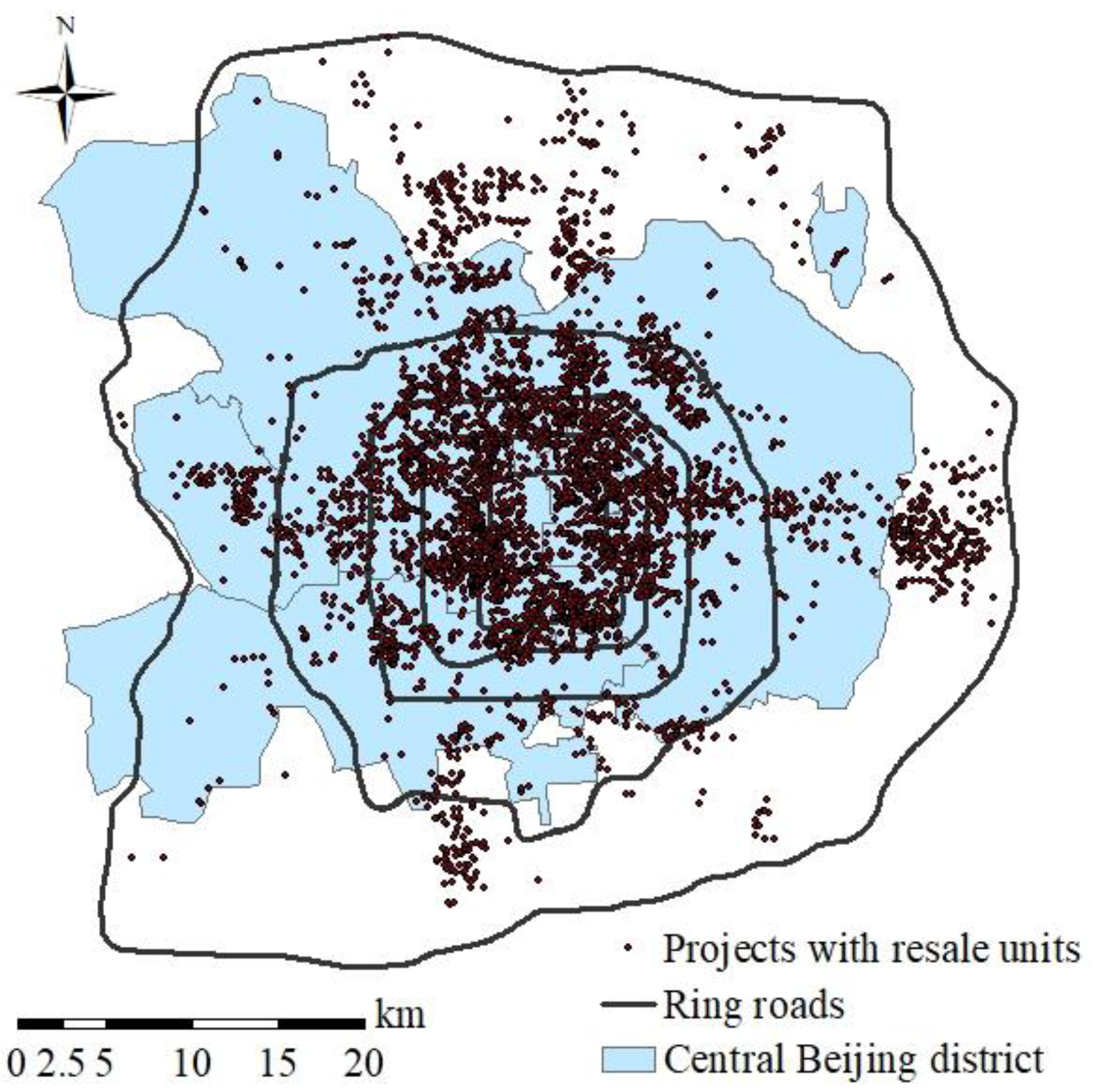
WoAiWoJia”, in Beijing. During our “clean” period from 11 January 2010 to 28 September 2010, the sample contains 5295 resale transactions covering more than 1477 residential complexes (housing development in Chinese cities typically occurs at a large scale and with a high degree of homogeneity within a residential “complex”, and a complex usually contains hundreds or even thousands of units with the same location, architectural design, structure, appliances and finishes), which are distributed all over Beijing. Figure 1 shows the spatial distribution of all the resale transactions in our dataset.
For each transaction, we have detailed information on both the real price (price_real) and the contract price (price_con), so we can observe the extent to which buyers engaged in Yin and Yang contracts. In addition, we have the following key information: address, unit size (size), level of decoration (decoration, decoration = 1 denotes undecorated houses, decoration = 2 indicates simply decorated ones, decoration = 3 indicates moderately decorated houses and decoration = 4 indicates well decorated houses), the orientation of the house (towards, according to the traditional preference of Chinese buyers, houses facing south or southeast are the best, towards = 2, followed by west, east or southwest, towards = 1, and the worst is north, towards = 0), on which floor the housing is located (floor) and whether the housing is on the top floor (top). By geo-coding all resales on Beijing’s GIS map, we construct several location measures for each residential complex, including the distance from each residential complex to the city center (d_CBD) and whether the complex is within 2 km of a “key” primary school (school) or a “Grade-A” hospital (hospital) and within 1 km of a subway stop (subway). The different thresholds are because a reasonable “walkable” distance to key public infrastructures such as hospitals and subway stations is 1 km [50]; however, the school districts of key primary schools are usually the surrounding area, i.e., within 2 km of the corresponding school. Summary statistics are provided in Table 2.

3.1. Patterns of Yin and Yang Contracts

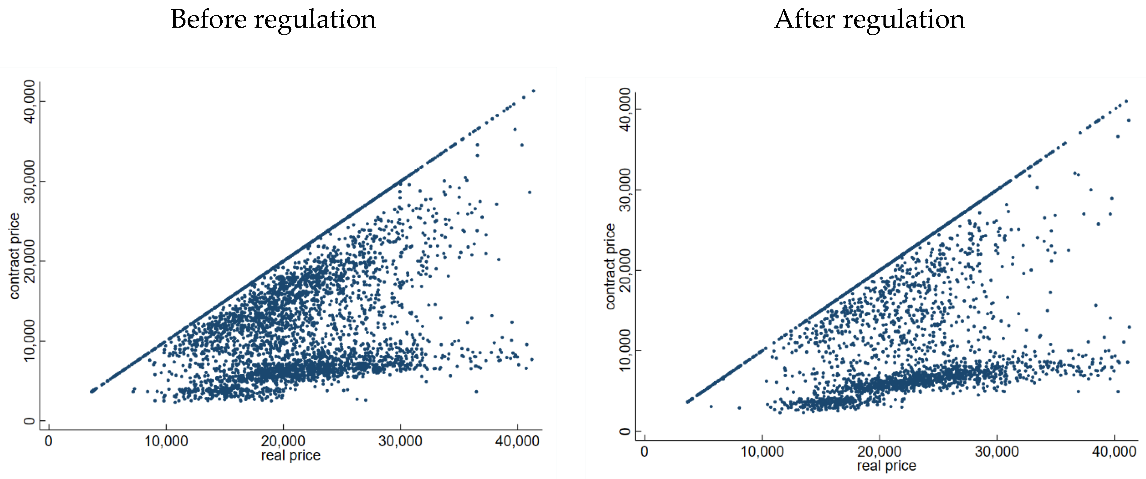
According to our sample, the real price was 15,610 RMB/m2 on average in the period of 2005–2011, while the contract price was only 8958 RMB/m2, which is 57% of the former. We focus on the clean window before and after the 2010 regulation and scatter the two prices of each transaction in Figure 2, with the real price on the horizonal axis and the contract price on the vertical axis. The left panel shows transactions before the regulation implementation, while the right panel includes those after. Obviously, the contract price is not higher than the real price for each micro transaction over the sample period. When comparing the two panels, we find that the transaction volume after the regulation is much less than before, and the proportion of samples with a higher price gap is much larger. On average, the real price is 1.58 times the contract price before the regulation and 1.98 times after.

3.2. Trends of “Yin-and-Yang” Contracts before and after Regulation

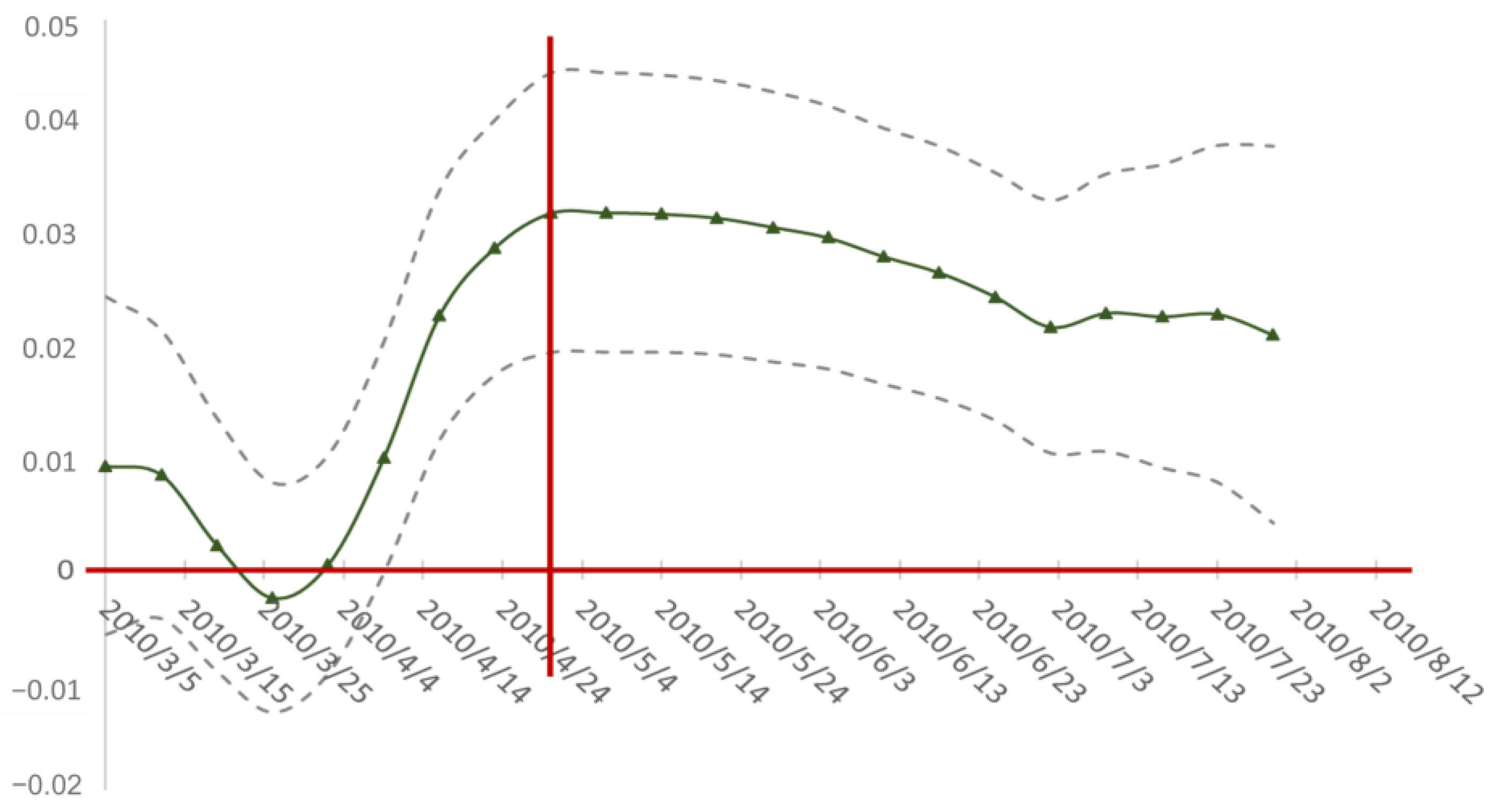
For each transaction, we define a new variable, price gap (pricegap), as the ratio of the real price to the contract price. The higher the value of this variable, the greater the difference between the actual transaction price and the contract price. Figure 3 scatters the weekly average. After the implementation of the house-purchasing regulation (referred to as “HPR” in the following sections), the gap between the two prices initially drops sharply but then increases at a faster rate. The price difference returns to the original gap level in approximately 6 weeks and continues to rise at the higher growth rate. This pattern is quantitively described in the empirical section.
Interestingly, the extent of under-reporting eases shortly after the regulation and then quickly recovers. Recall that Yin-and-Yang contracts are used to save tax at the cost of a higher one-time payment. When the amount of value-added tax is decreased due to a lower premium over the previous sale, buyers are willing to sign a higher contract price to relieve liquidity pressure. However, we cannot observe the repeat-sale samples directly from our data, which means we are unable to test this quantitively. Hence, we provide a rough estimation of the premium over the previous sale: by week and by residential complex, we calculate the average premium over its average price of 1 year before, 2 years before, 3 years before and 4 years before. We plot a city-wide average premium in Figure 4.
The four panels in Figure 4 are very similar in their patterns: the average premium drops sharply immediately after regulation and then recovers quickly, which is consistent with the trend of housing prices after regulation (Sun et al., 2017). Therefore, we infer that in the short period when the premium over the last sale decreases, buyers are less willing to under-report than they are thereafter, which leads the price spread (pricegap) to drop temporarily, as shown in Figure 3.

3.3. Patterns of Houses’ Key Features before and after the Regulation

One concern is that the housing market may experience some structural changes in the physical or location attributes of transacted houses after regulation. If the change in the price difference of the real price and the contract-recorded disclosed price in this article reveals the abovementioned changes rather than the payment transformation of home buyers, we first intuitively observe the data distribution of the physical and locational attributes of these microtransactions as well as their prices before and after the purchase restriction policies, as shown in Figure 5. The figure in the top left indicates that the distribution of the real price shifted to the right significantly after regulation; in other words, the transaction prices became higher. In contrast, transactions with lower contract prices accounted for a larger proportion after the HPR, as shown by the figure in the top right. The figures in the bottom panel reveal that the distribution of two key physical and locational attributes, unit size (size) and distance to the city center (d_CBD), show little change. Therefore, we believe the following empirical results are not induced by the structural changes of resale transactions’ physical or locational features.

4. Empirical Strategy

4.1. Cheating When Regulated

To reveal the more severe cheating under strict regulation in which market participants attempt to avoid regulation by further under-reporting the transaction price, we observe the gap between the real price and the contract price (pricegap) and its trend before and after regulation. A critical concern is that there may be time-varying omitted variables. In this paper, we employ three methods to eliminate this concern. First, we conduct our empirical studies based on a clean time window with only the targeted housing market regulations. Second, we pay special attention to differentiated effects that only result from the policy itself instead of any omitted factors. Third, we conduct two placebo tests and find no similar phenomenon around other cutoff time points.

4.1.1. Baseline Regressions

We choose a clean time window during which the only housing-market policies are regulations implemented on 30 April 2010. The previous policy on Beijing’s housing market took place on 10 January 2010, and the next was on 29 September 2010; hence, our time window is from 11 January 2010 to 28 September 2010. We employ a hedonic function to capture the price difference as in Equation (1):
log ( pricegap i t ) = α 0 + α 1 X i + α 2 L i + α 3 T + α 4 H P R + α 5 H P R × T + μ
where pricegapit is the difference between the real price and the contract price for transaction i occurring at time t, which is calculated as the real price divided by the contract price. Xi is a vector of the physical attributes of the housing transaction, including the house size (size), the decoration status (decoration), the house orientation (towards), the house age (age), the floor where the house is located (floor) and whether the house is on the top floor (top). Li is a vector of the locational attributes of the housing unit, including the distance to the city center (d_CBD), whether the house is within 2 km of a key primary school (keyschool), and whether the house is within 1 km of a subway station (subway) and a “3-A” hospital (hospital). HPR is a dummy variable denoting whether the transaction occurs after the implementation of the house-purchasing regulations in April 2010. T is defined as the Tth week of policy implementation, which captures the time trend of under-reporting. We use the linear weekly trend as the baseline and second-order and third-order weekly polynomial functions of time trends as robustness checks.
We expect the coefficient of HPR × T to be positive, which indicates a rapidly growing price gap in “Yin-and-Yang” contracts, meaning that buyers are further cheating on housing transaction prices under strict regulation. This trend can be qualitatively observed in Figure 3. However, the sign of α 4 may be ambiguous, and the explanation is much more complicated. According to Figure 4, buyers were motivated to narrow the price spread shortly after the policy because the transaction prices were temporarily reduced by the most stringent regulation (Sun et al., 2017) so that the tax burden was eased and buyers were less motivated to under-report in this short period. The short-run effect of regulation on “Yin-and-Yang” contracts is captured by α 4 + α 4 × T and may be negative when T is small; thus, we expect α4, the coefficient of HPR, to be negative or at least not significantly positive.
We further consider a heterogeneous impact of regulations as in Equation (2), where size90 denotes whether the transacted housing unit is larger than 90 m2 (1 = YES). Houses larger than 90 m2 are more likely to be treated because smaller houses can be exempt from a higher ratio of down payment if they are the buyer’s first home, according to the policy rules. The more the government regulates transactions, the keener buyers are to sign “Yin-and-Yang” contracts. Thus, we expect that the coefficient of HPR × T × size90 is also positive.
log ( pricegap i t ) = α 0 + α 1 X i + α 2 L i + α 3 T + α 4 H P R + α 5 H P R × T   + α 6 H P R × T × s i z e 90 + α 7 s i z e 90 + α 8 H P R × s i z e 90   + α 9 T × s i z e 90 + μ
We note that because the heterogeneity between the two groups is manually set by the 2010 regulation, the significant coefficient of HPR × T × size90 also confirms that the positive break in the trend of the price gap results from this policy instead of any potential time-varying omitted variables.

4.1.2. Robustness Checks

First, there may be concerns that the trends are dominated by the intensive margin, which means that those engaged in “Yin-and-Yang” contracts under-report a lower price while more buyers no longer cheat. Therefore, we conduct similar regressions as in Equations (1) and (2), but replace the dependent variable with a dummy D (pricegap > 1), which equals 1 when buyers are under-reporting and 0 otherwise, to test the trend on the extensive margin. We also predict the coefficients of interaction terms to be significantly positive, meaning that more transactions involve “Yin-and-Yang” contracts after regulation.
Second, we adjust the identification by changing the length of our sample period to a symmetric window that is 4 weeks both before and after the regulations and 8 weeks and 12 weeks, respectively. We also change the linear weekly trend into second-order and third-order polynomial functions of weekly trends. We continue to find a positive break in the trend of “Yin-and-Yang” contracts.
Third, we conduct two placebo tests, one each day of our sample period, as a hypothetical cutoff and repeating the regressions of Equations (1) and (2) and the other repeating the baseline regressions in the previous and next year, respectively, with the same date of the year as the cutoff point.
Finally, we duplicate the regressions for another regulation implemented on 27 September 2009 (referred to as “927 policies” below), when the government also tightened the liquidity of home buyers but made no distinction among house sizes. Thus, we expect buyers to cheat on the transaction prices as they did under the 2010 regulations, but there should be no difference among home-buyers of difference house sizes.

4.2. Enlarged Inequality from Cheating under Regulation

The regressions in Equations (1) and (2) aim to investigate the faster-growing trend of the price gap after the most stringent regulation implemented in April 2010, which proves that buyers are further cheating on transaction prices. As mentioned in Section 2, under-reporting the transaction price saves tax at the cost of higher one-time payments. Hence, the faster-growing trend of the price gap may imply that the average liquidity constraints are easier on the market. Considering that tightened financing is included in the housing market regulation, there may be a structural evolution in home buyers in which households with higher liquidity pressure are replaced by those with sufficient money, which can be inferred as enlarged inequality. We provide more evidence on this issue in this section.
First, we try to infer the relationship between “Yin-and-Yang” contracts and buyers’ liquidity through the differences in house size. An enlarged price gap may be attributed to either a higher real price or a lower contract price or to disproportional growth of the two, each of which means quite different things for buyers and challenges our inference about the liquidity issue. Specifically, a lower contract price combined with an unchanged or even higher real price imposes much higher liquidity pressure on buyers and implies an evolution in home-buyers in which liquidity-constrained households are crowded out and less-constrained households flow in. However, any downward trend in the real price will expand the space to reduce the contract price for buyers, which may contradict our hypothesis. We attempt to find the exact reason for the enlarged price gap by investigating the changes in trends for real and contract prices. Specifically, we replace the dependent variable in Equations (1) and (2) with log (real_priceit) and log (contract_priceit) and repeat the baseline regressions as above.
Furthermore, we link buyers’ decisions on “Yin-and-Yang” contracts with their liquidity status. Considering houses’ dual role in investment and consumption, a considerable percentage of buyers’ down payment comes from the proceeds on the sale of their old homes, especially for immigrants [51]. Therefore, we attempt to group buyers according to the value of their old homes. The more valuable their old homes are, the higher liquidity they will have to under-report the transaction price. Because we do not have detailed information on buyers’ income or household assets, we proxy the value of their old homes with the average housing price of their home city. Note that we exclude native Beijing residents. We split the sample into two groups according to the median value of the housing prices of the buyers’ birth cities and replicate the regressions in Equations (1) and (2). We expect the enlarged price gap to be more pronounced for buyers whose old homes have higher value.
Finally, we repeat the regressions for another housing-market-related regulation carried out on 26 January 2011 (referred to as “HPR2011” below) to confirm our suggestion that households with less liquidity pressure gradually crowd out those with higher liquidity constraints after regulation. Having shown that home-buyers further under-report their transaction price to avoid regulation and that this cheating behavior is closely related to their liquidity pressure, we continue to show that if wealthier buyers (those with more sufficient liquidity) are blocked from the housing market, we should not observe a similar phenomenon as above. Compared to the 2010 regulations, the 2011 regulation implements a stricter policy to prohibit households from buying a third home, which can block wealthy families from the housing market; thus, survivors may have less willingness to enlarge the price gap than in 2010. Therefore, we expect the coefficients of HPR2011 × T and HPR2011 × T × size90 to no longer be significantly positive for the 2011 regulation.

5. Empirical Results

5.1. Cheating When Regulated

We first investigate whether buyers are further cheating after the implementation of the house-purchasing regulation. Taking the difference between the real price and the contract price (pricegap = real price/contract price) as the dependent variable, Table 3 presents the estimation results for Equation (1). Here, we employ a clean time window during which the regulation implemented on 30 April 2010, is the only exogenous policy shock, so we can avoid potential time-varying omitted variable concerns.
In Column (1), we include only the physical and locational attributes of houses as control variables. We then add the buyer’s birth city fixed effect and season fixed effect in the regressions in Columns (2) and (3), respectively, and include both in Column (4). Our key coefficients remain statistically significant and almost unchanged quantitatively. Specifically, the coefficient of the interaction term between the regulation dummy (HPR) and the linear weekly trend (T) is significantly positive at the 1% level, implying that buyers cheat on the contract price to an increasing extent after regulation. The magnitude of the coefficient is worth noting. Recall that the mean value of the variable pricegap is 2.26 in our sample period, meaning that the real price is, on average, 2.26 times the corresponding contract price. This multiple increases by 3.24% every week after regulation, as indicated by the coefficient of HPR × T in Column (4). In addition, the coefficients of the regulation dummy (HPR) are significantly negative in the four columns, which is also consistent with our expectation. However, this downward jump is offset in six weeks when more buyers engage in “Yin-and-Yang” contracts to an increasing extent over time.
We further use the intentional difference in policy exposure of different houses to mitigate the potential missing-variable concerns. As previously stated, houses smaller than 90 m2 could be exempted from some part of the transaction tax if they are the first house of the buyer, which makes houses larger than 90 m2 more likely to be exposed to the regulation. Table 4 reports the heterogeneous responses of the price gap to the regulation as in Equation (2). In the four columns, the coefficients of both HPR × T and HPR × T × size90 are positive and statistically significant, as expected, revealing that the impact of the regulation is more pronounced on houses that are more likely to be regulated. Quantitatively, the coefficient of HPR × T × size90 is 0.080 in Column (4), which is twice that of HPR × T, suggesting that the price gap for larger houses is growing twice as fast as that of smaller ones. The above results confirm that the enlarged growth rate of the price gap resulted from the 2010 regulations instead of potential omitted variables during this period because differentiated provisions on the two groups are manually set by this policy.

5.2. Robustness Checks

5.2.1. Extensive Margins on “Yin-and-Yang” Contracts

A potential concern regarding the increasing price gap of “Yin-and-Yang” contracts comes from the intensive margin, whereby those who intend to cheat are cheating more on the transaction price instead of more buyers signing “Yin-and-Yang” contracts. Therefore, we replace the dependent variable of the baseline regressions with a dummy variable indicating whether the buyer is under-reporting to examine the extensive margin. As shown in Table 5, the coefficient of HPR × T is significantly positive in Column (1), which means the probability of signing a “Yin-and-Yang” contract also demonstrates a positive break in the trend after regulation, and the effect is large enough to offset the downward jump in 4 weeks. We also differentiate the responses of larger houses to smaller ones in Column (2), whereby houses larger than 90 m2, which are more exposed to regulation, have “Yin-and-Yang” contracts with a faster-growing price spread. Therefore, we can conclude that buyers are not only more like to engage in a “Yin-and-Yang” contract after regulation (on the extensive margin) but also to cheat on the transaction price to a greater extent (on the intensive margin).

5.2.2. Alternate Time Window and the Polynomial Trend

Now, we check whether the baseline results are robust to alternative empirical specifications. We first consider changing the time window around the regulation and report the results in Table 6. In Columns (1) and (2), we replicate the baseline regressions but consider a ±4-week window. The regression results are in line with those in Table 3 and Table 4. We also adjust the time windows to ±8 weeks and ±12 weeks, and as shown in Columns (3)–(6), our main results still hold. Thus, employing different time windows does not affect our findings in the baseline regressions.
We then replace the linear weekly trend with different orders of polynomial trends because they may better characterize the variation of the price difference before and after the regulation. Table 7 presents the regression results. Specifically, we consider the quadratic trend in Columns (1) and (2) and the cubic trend in Columns (3) and (4). We consistently find significantly positive coefficients on the interactions between HPR and polynomial trends as well as the triple interaction terms. These findings are still in favor of our hypotheses.

5.2.3. Placebo Tests

Nevertheless, we may question whether the key coefficients in Table 3 and Table 4 simply capture some unobserved shocks during our sample period that happen to be more pronounced in larger houses. Thus, we employ two placebo tests to examine whether alternative pivot weeks generate similar results as the baseline regressions.
First, each week of our sample period is taken as the hypothetical policy implementation week in turn, and we repeat the baseline regression 22 times. The coefficients on HPR × T and HPR × T × size90 from these regressions are plotted in Figure 6 and Figure 7 along with their 95% confidence intervals. Obviously, both figures confirm that the trend of the price difference changes sharply in the week the regulation is actually implemented, which means that further under-reporting of the transaction price is indeed generated by the stringent regulation instead of any potential unobserved factors.
Second, we shift the sample period one year forward and backward, taking 30 April 2009 and 30 April 2011 as the hypothetical cutoff time points. With the same specifications employed in the baseline regressions, the results are reported in Table 8. We find no significant break in the price gap trend for either 2009 or 2011 nor for either smaller or larger houses.

5.2.4. Testing the Effects of Another Regulation Policy

Finally, we employ the same specifications to estimate the impact of another regulation implemented on 27 September 2007 (“927 policies”). The mortgage rate was increased by the 927 policies, leading to an increase in the opportunity cost of loans. As stated in Section 2.2, buyers would be motivated to enlarge the price difference as well. However, the 927 policies make no distinction among houses of different sizes; thus, the enlarged price difference should not show any distinction with regard to house size. The regression results reported in Table 9 support our predictions above. The coefficient of HPR927 × T in Column (1) is significantly positive, indicating that the 927 policies produced a similar break of the price difference trend as the 2010 regulations. However, when we further examine the price difference trend among different house sizes, the coefficient of HPR927 × T × size90 in Column (2) is not significant, showing a consistent trend of price difference among all house sizes.
In summary, the above checks lead to the robust conclusion that the difference between the real price and the contract price increased more rapidly after the implementation of the 2010 regulations, as revealed in the baseline regressions. This means that buyers attempt to avoid regulation by further under-reporting the transaction price. In the following sections, we provide evidence on potential outcomes of this further cheating, such as the possibility of enlarged inequality and a considerable amount of extra tax loss.

5.3. Enlarged Inequality

Having shown that buyers under-report their housing transaction prices to an increasing extent under strict regulation, we continue to reveal the relationship between “Yin-and-Yang” contracts and buyers’ liquidity conditions and the resulting inequality issues. We note that Yin-and-Yang contracts impose great liquidity pressure on buyers, despite helping to avoid stringent regulations, which may shut some households out of the housing market and lead to more inequality. In this section, we provide evidence on the enlarged inequality when “rich” households further engage in Yin-and-Yang contracts under stringent regulation while those without sufficient liquidity cannot. The key problem here is that we do not have detailed information about buyers, such as their income or wealth, so we must make some inferences based on different aspects.
We first emphasize that all house buyers face higher liquidity pressure after regulation, regardless of whether they are exposed to the policy. We divide the price difference into the real price and the contract price and explore their responses to housing price regulation, respectively. The estimation results are reported in Table 10. The coefficient of HPR × T is significantly positive in Column (1) but is not significant in Column (2), while the coefficient of HPR × T × size90 in Column (2) is positive and statistically significant, implying that the real price trend break is mainly driven by transactions of houses larger than 90 m2. Interestingly, as shown in Columns (3) and (4), the contract price of small houses exhibits a downward trend, while that of large houses displays an upward trend, but not as much as their relative real price. Therefore, we can infer that for houses smaller than 90 m2, buyers pay roughly the same total price after regulation but with a higher down payment due to a lower contract price. For larger houses, buyers pay a higher total price after regulation. When we further account for the larger increase of the real price than the contract price, the down payment is even higher. This means that buyers of all houses face more liquidity pressure after regulation; thus, households without sufficient liquidity may be shut out of the market.
Second, we examine the link between buyers’ under-reporting and their liquidity by comparing households with different levels of liquidity constraints. A key challenge here is that we do not have detailed information about buyers’ income or assets due to the privacy protection rules of the broker. As mentioned previously, selling a house in one’s hometown is a key means of financing to purchase a home in Beijing for immigrants. Thus, we focus on non-native buyers and measure their liquidity constraints according to the housing prices of their birth city. In Table 11, we split the observations into two groups according to the median value of the average housing price of buyers’ birth cities and check the impact of the regulations for both groups. The coefficients of HPR × T and HPR × T × size90 are not significant in Columns (1) and (2), while they are all significantly positive in Columns (3) and (4), meaning that families with less liquidity constraints are more likely to further enlarge the price gap in their “Yin-and-Yang” contracts. We can easily infer that under the circumstances in which all other buyers are engaged in “Yin-and-Yang” contracts with a large price spread to avoid regulation, those who cannot do so are gradually crowded out of the market.
Thus far, we have claimed that there may have been an evolution of buyers on the housing market after the implementation of the 2010 regulations as families with higher liquidity constraints were crowed out and those with abundant cash flowed in. This phenomenon may disappear if the inflow of wealthy families is prohibited. To test this hypothesis, we focus on another regulation implemented in January 2011, when purchasing a third home was strictly forbidden. Compared to the 2010 regulations, the 2011 regulations blocked more wealthy families from the housing market; thus, survivors may have been less willing to enlarge the price gap than they would have been in 2010. We replicate our baseline regressions with the implementation of the 2011 regulation as the cutoff, and the results are reported in Table 12. The coefficients of both HPR × T and HPR × T × size90 are not significant, showing a quite different pattern from the enlarged inequality resulting from the 2010 regulations.

6. An Estimation of Extra Tax Loss

In addition to the enlarged inequality issues stated in the previous section, further cheating on transaction price leads to extra tax loss to the government, which may be ignored when evaluating the policy outcomes. In this section, we conduct a counterfactual estimation of this extra tax loss according to our baseline regressions and find it quite considerable even compared to Beijing’s total government revenue.
Under-reporting of the transaction price for the purpose of saving tax has been widely observed on the housing market and resulted in great tax loss. We take this as the default and attempt to calculate how much extra tax loss has been caused by the greater extent of cheating after regulation. We graph the real price, the predicted contract price and a counterfactual contract price (we predict the counter-factual contract price based on our empirical results by letting HPR = 0), as shown in Figure 8. The solid line in blue shows the weekly average real price per square meter, which drops temporarily 2–3 weeks after regulation but recovers quickly. The long-dashed line in red represents the predicted contract price when buyers are under-reporting the transaction price to an increasing extent to avoid regulation, as revealed in our baseline regression. The short-dashed line in green denotes our counterfactual estimated contract price, or what the contract price would be if there were no regulations or if people did not cheat more to avoid regulation.
The gap between the solid blue line and the short-dashed green line implies a tax loss when buyers under-report only to evade transaction tax, and the gap between the short-dashed green line and the long-dashed red line implies an extra tax loss when buyers attempt to avoid regulation by further cheating. The former is almost constant, while the latter gap is zero before the regulation but enlarges quickly thereafter.
To estimate the amount of extra tax loss from further under-reporting of transaction prices, we multiply the above price gaps by the tax rate for house resales in Beijing in 2010, as shown in Figure 9. The blue solid line graphs the estimated tax loss of Yin-and-Yang contracts with the purpose of saving tax but without any incentive to avoid house-purchasing regulation, which we find to be approximately constant at approximately 20,000 RMB per transaction. The red dashed line shows the extra tax loss when buyers further under-report the price to avoid regulation: it is zero before the implementation of regulation but grows quickly and reaches 40,000 RMB per transaction.
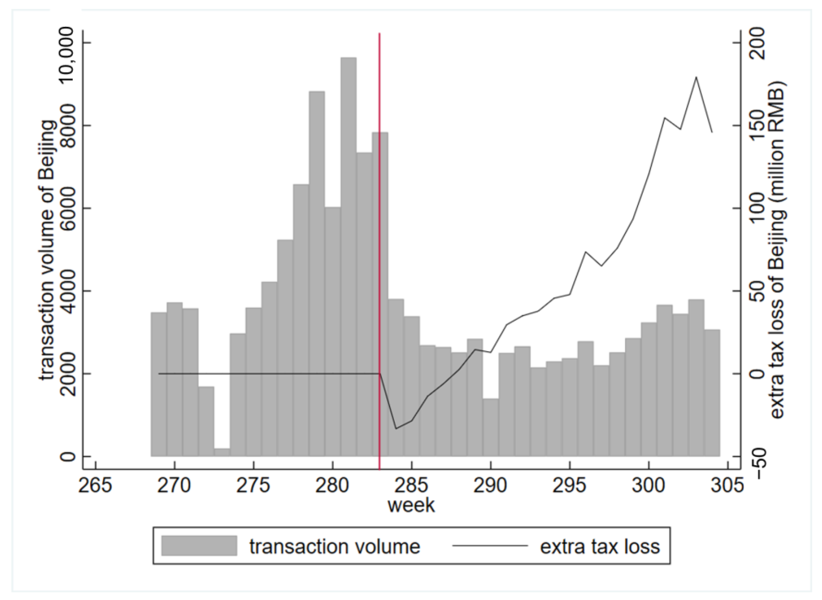
To move forward, we combine the extra tax loss of each transaction and the transaction volumes of Beijing in Figure 10 so that we can estimate the total amount of tax loss. In our clean time window, the Beijing government loses an extra 58 million RMB from people further cheating each week after regulation. Given that the monthly fiscal revenue of Beijing within our time window varies from 15 to 22 billion RMB, the extra tax loss after stringent regulation is considerably large, accounting for approximately 1–1.5% of the government’s total fiscal income. It is worth noting that we take the tax loss from “Yin-and-Yang” contracts as the default and estimate the extra loss from an even lower contract price with regulation. We find that the extra price gap approximately equals the initial price gap without any further incentive to avoid regulation. Thus, the total loss from Yin-and-Yang contracts in housing resales almost accounts for 2–3% of Beijing’s fiscal revenue.

7. Conclusions and Implications

This paper studies the price difference in Yin-and-Yang contracts on the housing market and investigates how price differences grow before and after the implementation of stringent regulation. Despite the initial purpose of reducing transaction-based tax, the market participants further under-report the transaction price to evade regulations. Because Yin-and-Yang contracts and strict regulations both impose liquidity pressure on buyers, we note that the faster-growing price gap implies an inflow of less liquidity-constrained households and a crowding out of more constrained ones on the housing market, which is also a signal of enlarged inequality after regulation.
Empirically, we find a positive break in the linear trend of the price gap with the implementation of regulations, which is more pronounced for houses with a higher probability to be treated and for households with less liquidity constraints. The faster-growing process is prevented if new purchases by richer households are strictly prohibited. We also attempt to estimate the extra tax loss when buyers further under-report the transaction price to evade regulation.
As the first paper to emphasize Yin-and-Yang contracts on the housing market and to use them as an opportunity to observe the enlarged inequality of regulation, this paper has meaningful implications. First, when investigating any policies or events that may affect housing prices, attention should be paid to the actual transaction price, which may be disguised by Yin-and-Yang contracts, leading to a bias in empirical studies. Second, this paper sheds light on the side effects of regulations on the housing market that lead to non-price allocation mechanisms and enlarged inequality, similar to regulations in the other fields, which may even fail directly in controlling prices with the presence of market participants’ cheating behavior.

Author Contributions

Conceptualization, Y.D.; methodology, Y.D.; validation, Y.D.; writing—original draft preparation, Y.X.; writing—review and editing, Y.X.; visualization, Y.X.; funding acquisition, Y.X. All authors have read and agreed to the published version of the manuscript.

Funding

Yangfei Xu acknowledges support from the National Natural Science Foundation of China (#71804107).

Institutional Review Board Statement

Not applicable.

Informed Consent Statement

Not applicable.

Data Availability Statement

The data presented in this study are available only in this article. Please request from the authors if necessary.

Conflicts of Interest

The authors declare no conflict of interest.

Appendix A

Figure A1. World-wide novel research that is related to our research question.
Sustainability 14 13346 g0a1

References

  1. Cao, J. The Chinese Real Estate Market: Development, Regulation and Investment; Routledge: London, UK, 2015. [Google Scholar]
  2. Glaeser, E.; Huang, W.; Ma, Y.; Shleifer, A. A real estate boom with Chinese characteristics. J. Econ. Perspect. 2017, 31, 93–116. [Google Scholar] [CrossRef] [Green Version]
  3. Du, Z.; Zhang, L. Home-purchase restriction, property tax and housing price in China: A counterfactual analysis. J. Econom. 2015, 188, 558–568. [Google Scholar] [CrossRef]
  4. Sun, W.; Zheng, S.; Geltner, D.M.; Wang, R. The housing market effects of local home purchase restrictions: Evidence from Beijing. J. Real Estate Financ. Econ. 2017, 55, 288–312. [Google Scholar] [CrossRef]
  5. Jia, S.; Wang, Y.; Fan, G.-Z. Home-purchase limits and housing prices: Evidence from China. J. Real Estate Financ. Econ. 2018, 56, 386–409. [Google Scholar] [CrossRef]
  6. Cao, X.; Huang, B.; Lai, R.N. The Impact of Exogenous Demand Shock on the Housing Market: Evidence from the Home Purchase Restriction Policy in the People’s Republic of China.2018. Available online: http://hdl.handle.net/10419/190245 (accessed on 1 October 2022).
  7. Chen, Z.; Wang, C. Effects of intervention policies on speculation in housing market: Evidence from China. J. Manag. Sci. Eng. 2022, 7, 233–242. [Google Scholar] [CrossRef]
  8. Leung, C.K.; Leung, T.C.; Tsang, K. Tax-driven bunching of housing market transactions: The case of Hong Kong. Int. Real Estate Rev. 2015, 18, 473–501. [Google Scholar] [CrossRef]
  9. Agarwal, S.; Li, K.; Qin, Y.; Wu, J.; Yan, J. Tax evasion, capital gains taxes, and the housing market. J. Public Econ. 2020, 188, 104222. [Google Scholar] [CrossRef]
  10. Li, V.J.; Cheng, A.W.W.; Cheong, T.S. Home purchase restriction and housing price: A distribution dynamics analysis. Reg. Sci. Urban Econ. 2017, 67, 1–10. [Google Scholar] [CrossRef]
  11. Wu, Y.; Li, Y. Impact of government intervention in the housing market: Evidence from the housing purchase restriction policy in China. Appl. Econ. 2018, 50, 691–705. [Google Scholar] [CrossRef]
  12. Li, Y.; Zhu, D.; Zhao, J.; Zheng, X.; Zhang, L. Effect of the housing purchase restriction policy on the Real Estate Market: Evidence from a typical suburb of Beijing, China. Land Use Policy 2020, 94, 104528. [Google Scholar] [CrossRef]
  13. Friedman, M.; Stigler, G.J. Roofs or Ceilings? The Current Housing Problem; Foundation for Economic Education: New York, NY, USA, 1946. [Google Scholar]
  14. Glaeser, E.L.; Luttmer, E.F. The misallocation of housing under rent control. Am. Econ. Rev. 2003, 93, 1027–1046. [Google Scholar] [CrossRef] [Green Version]
  15. Bardey, D.; Bommier, A.; Jullien, B. Retail price regulation and innovation: Reference pricing in the pharmaceutical industry. J. Health Econ. 2010, 29, 303–316. [Google Scholar] [CrossRef] [Green Version]
  16. Golec, J.; Hegde, S.; Vernon, J.A. Pharmaceutical R & D spending and threats of price regulation. J. Financ. Quant. Anal. 2010, 45, 239–264. [Google Scholar] [CrossRef]
  17. Davis, L.W.; Kilian, L. The allocative cost of price ceilings in the US residential market for natural gas. J. Political Econ. 2011, 119, 212–241. [Google Scholar] [CrossRef] [Green Version]
  18. Gyourko, J.; Linneman, P. Equity and efficiency aspects of rent control: An empirical study of New York City. J. Urban Econ. 1989, 26, 54–74. [Google Scholar] [CrossRef]
  19. Sims, D.P. Out of control: What can we learn from the end of Massachusetts rent control? J. Urban Econ. 2007, 61, 129–151. [Google Scholar] [CrossRef]
  20. Arnott, R.; Shevyakhova, E. Tenancy rent control and credible commitment in maintenance. Reg. Sci. Urban Econ. 2014, 47, 72–85. [Google Scholar] [CrossRef] [Green Version]
  21. Eriksen, M.D.; Rosenthal, S.S. Crowd out effects of place-based subsidized rental housing: New evidence from the LIHTC program. J. Public Econ. 2010, 94, 953–966. [Google Scholar] [CrossRef]
  22. Jacob, B.A.; Ludwig, J. The effects of housing assistance on labor supply: Evidence from a voucher lottery. Am. Econ. Rev. 2012, 102, 272–304. [Google Scholar] [CrossRef] [Green Version]
  23. Öst, C.E.; Söderberg, B.; Wilhelmsson, M. Household allocation and spatial distribution in a market under (“soft”) rent control. J. Policy Model. 2014, 36, 353–372. [Google Scholar] [CrossRef]
  24. Cao, J.A.; Keivani, R. The limits and potentials of the housing market enabling paradigm: An evaluation of China’s housing policies from 1998 to 2011. Hous. Stud. 2014, 29, 44–68. [Google Scholar] [CrossRef]
  25. Chisholm, E.; Howden-Chapman, P.; Fougere, G. Tenants’ responses to substandard housing: Hidden and invisible power and the failure of rental housing regulation. Hous. Theory Soc. 2020, 37, 139–161. [Google Scholar] [CrossRef]
  26. Kettunen, H.; Ruonavaara, H. Rent regulation in 21st century Europe. Comparative perspectives. Hous. Stud. 2021, 36, 1446–1468. [Google Scholar] [CrossRef]
  27. Mian, A.; Sufi, A. The consequences of mortgage credit expansion: Evidence from the US mortgage default crisis. Q. J. Econ. 2009, 124, 1449–1496. [Google Scholar] [CrossRef]
  28. Favara, G.; Imbs, J. Credit supply and the price of housing. Am. Econ. Rev. 2015, 105, 958–992. [Google Scholar] [CrossRef] [Green Version]
  29. Glaeser, E.L.; Nathanson, C.G. Housing bubbles. In Handbook of Regional and Urban Economics; Elsevier: Amsterdam, The Netherlands, 2015; Volume 5, pp. 701–751. [Google Scholar] [CrossRef]
  30. Davis, M.A.; Van Nieuwerburgh, S. Housing, finance, and the macroeconomy. In Handbook of Regional and Urban Economics; Elsevier: Amsterdam, The Netherlands, 2015; Volume 5, pp. 753–811. [Google Scholar] [CrossRef]
  31. Silos, P. Housing, portfolio choice and the macroeconomy. J. Econ. Dyn. Control 2007, 31, 2774–2801. [Google Scholar] [CrossRef]
  32. Chambers, M.; Garriga, C.; Schlagenhauf, D.E. Accounting for changes in the homeownership rate. Int. Econ. Rev. 2009, 50, 677–726. [Google Scholar] [CrossRef] [Green Version]
  33. Cunningham, C.R.; Engelhardt, G.V. Housing capital-gains taxation and homeowner mobility: Evidence from the Taxpayer Relief Act of 1997. J. Urban Econ. 2008, 63, 803–815. [Google Scholar] [CrossRef]
  34. Dachis, B.; Duranton, G.; Turner, M.A. The effects of land transfer taxes on real estate markets: Evidence from a natural experiment in Toronto. J. Econ. Geogr. 2012, 12, 327–354. [Google Scholar] [CrossRef] [Green Version]
  35. Best, M.C.; Kleven, H.J. Housing market responses to transaction taxes: Evidence from notches and stimulus in the UK. Rev. Econ. Stud. 2018, 85, 157–193. [Google Scholar] [CrossRef]
  36. Verma, R.; Husain, R. The Resilience and Strength of the New Housing Market during the Pandemic; Statistics Canada/Statistique Canada: Ottawa, ON, Canada, 2020. [Google Scholar]
  37. Yang, M.; Zhou, J. The impact of COVID-19 on the housing market: Evidence from the Yangtze river delta region in China. Appl. Econ. Lett. 2022, 29, 409–412. [Google Scholar] [CrossRef]
  38. Hu, M.R.; Lee, A.D.; Zou, D. COVID-19 and housing prices: Australian evidence with daily hedonic returns. Financ. Res. Lett. 2021, 43, 101960. [Google Scholar] [CrossRef]
  39. Qian, X.; Qiu, S.; Zhang, G. The impact of COVID-19 on housing price: Evidence from China. Financ. Res. Lett. 2021, 43, 101944. [Google Scholar] [CrossRef]
  40. Arcaya, M.C.; Nidam, Y.; Binet, A.; Gibson, R.; Gavin, V. Rising home values and Covid-19 case rates in Massachusetts. Soc. Sci. Med. 2020, 265, 113290. [Google Scholar] [CrossRef]
  41. Wang, B. How does COVID-19 affect house prices? A cross-city analysis. J. Risk Financ. Manag. 2021, 14, 47. [Google Scholar] [CrossRef]
  42. Madeddu, M.; Clifford, B. Housing quality, permitted development and the role of regulation after COVID-19. Town Plan. Rev. 2021, 92, 41–48. [Google Scholar] [CrossRef]
  43. Kaklauskas, A.; Lepkova, N.; Raslanas, S.; Vetloviene, I.; Milevicius, V.; Sepliakov, J. COVID-19 and Green Housing: A Review of Relevant Literature. Energies 2021, 14, 2072. [Google Scholar] [CrossRef]
  44. Li, J.; Song, Q.; Peng, C.; Wu, Y. COVID-19 pandemic and household liquidity constraints: Evidence from micro data. Emerg. Mark. Financ. Trade 2020, 56, 3626–3634. [Google Scholar] [CrossRef]
  45. Brewer, M.; Tasseva, I.V. Did the UK policy response to Covid-19 protect household incomes? J. Econ. Inequal. 2021, 19, 433–458. [Google Scholar] [CrossRef]
  46. An, X.; Gabriel, S.A.; Tzur-Ilan, N. COVID-19 rental eviction moratoria and household well-being. Available online: https://www.researchgate.net/publication/349973336_COVID-19_Rental_Eviction_Moratoria_and_Household_Well-Being (accessed on 1 October 2022).
  47. Wu, J.; Gyourko, J.; Deng, Y. Evaluating conditions in major Chinese housing markets. Reg. Sci. Urban Econ. 2012, 42, 531–543. [Google Scholar] [CrossRef] [Green Version]
  48. Glaeser, E.L. A nation of gamblers: Real estate speculation and American history. Am. Econ. Rev. 2013, 103, 1–42. [Google Scholar] [CrossRef] [Green Version]
  49. Hansen, J.L.; Formby, J.P.; Smith, W.J. Estimating the income elasticity of demand for housing: A comparison of traditional and Lorenz-concentration curve methodologies. J. Hous. Econ. 1998, 7, 328–342. [Google Scholar] [CrossRef]
  50. Alshalalfah, B.; Shalaby, A. Relationship of walk access distance to transit with service, travel, and personal characteristics. J. Urban Plan. Dev. 2007, 133, 114–118. [Google Scholar] [CrossRef]
  51. Stein, J.C. Prices and trading volume in the housing market: A model with down-payment effects. Q. J. Econ. 1995, 110, 379–406. [Google Scholar] [CrossRef] [Green Version]
Figure 1. Spatial distribution of house resales. This figure plots the spatial distribution of our micro transaction samples. Beijing’s housing units are organized into “residential complexes”, each containing hundreds or even thousands of units. To protect buyers’ privacy, addresses are only provided at the complex level; thus, transactions in one complex share the same address and are represented by one dot in this figure. Our dataset contains transactions all over urban Beijing.
Sustainability 14 13346 g001
Figure 2. Comparison of real price and contract price. This figure scatters each transaction with the real price on the horizontal axis and the contract price on the vertical axis. We put transactions before the 2010 regulation in the left panel and those after regulation in the right panel. Obviously, the contract price is lower than the corresponding real price in most cases and is at least no more than the real price. In addition, the right panel shows a higher proportion of transactions for which the difference between the two prices is larger. Intuitively, this figure suggests that market participants under-report the transaction price to a greater extent after regulation.
Sustainability 14 13346 g002
Figure 3. Faster-growing gap between the real price and contract price. This figure plots the weekly average price gap (pricegap) between the real price and the contract price, which is defined as the real price divided by the contract price. We provide linear fitting lines for the pricegap before and after regulation. It is obvious that the spread between the real price and the contract price grows faster after regulation, which means, as this paper highlights, that market participants under-report the transaction price to an increasing extent. However, a remaining puzzle is that the price gap drops temporarily in the week of policy implementation. We provide a simple explanation in the following figure.
Sustainability 14 13346 g003
Figure 4. Average appreciation of resale houses with various turnover periods. We aim to exhibit the trend of housing price premiums from the last sale. Lacking detailed information on each resale for a house, we make some approximations. To proxy the premium from the previous sale 1 year before, we use the difference between a unit’s current transaction price and the weekly average price of the residential complex where the unit is located 1 year before the transaction. Proxies for the premium from 2 years before, 3 years before and 4 years before are constructed in the same way.
Sustainability 14 13346 g004
Figure 5. Distribution of several key variables before and after HPR. Figure 5 shows the data distribution of several key variables associated with the micro transactions, which are the real transaction price, the contract price, the house size and the distance to the city center, respectively. Compared to before the regulation, the distribution of real prices shifts to the right significantly, implying that the transaction price increases despite stringent regulations. The distribution of contract prices shifts to the left, indicating that market participants under-report the transaction price to an increasing extent. Both of these changes contribute to a larger gap between the real price and the contract price, and thus, impose a heavier liquidity pressure on buyers. However, the distributions of house size and distance to the city center do not demonstrate a significant shift before and after regulation, meaning that the change in “Yin-and-Yang” contracts does not result from a systematic evolution of houses transacted on the market.
Sustainability 14 13346 g005
Figure 6. Coefficients of HPR × T of placebo test I: regressions for hypothetical cutoffs. Figure 6 and Figure 7 plot the coefficients of key variables in our first placebo test. Our baseline regressions report that after the implementation of stringent regulations (on 30 April 2010), the gap between the real price and the contract price increases faster (revealed by the significantly positive coefficient of HPR × T), and the phenomenon is more pronounced for houses larger than 90 m2 (revealed by the significantly positive coefficient of HPR × T × size90). We take each date during our clean sample period as the cut-off time point in turn and repeat the baseline regressions; the coefficients of HPR × T are reported in this figure. We find that none of the hypothetical cut-off time points lead to a similar outcome as the actual cut-off.
Sustainability 14 13346 g006
Figure 7. Coefficients of HPR × T × size90 of placebo test I: regressions for hypothetical cutoffs. Figure 6 and Figure 7 plot the coefficients of key variables in our first placebo test. Our baseline regressions show that after the implementation of stringent regulations (on 30 April 2010), the gap between the real price and the contract price increases faster (revealed by the significantly positive coefficient of HPR × T), and the phenomenon is more pronounced for houses larger than 90 m2 (revealed by the significantly positive coefficient of HPR × T × size90). We take each date during our clean sample period as the cut-off time point in turn and repeat the baseline regressions; the coefficients of HPR × T × size90 are reported in this figure. We find that none of the hypothetical cut-off time points lead to a similar outcome as the actual cut-off.
Sustainability 14 13346 g007
Figure 8. Counterfactual estimation of contract price. We show the extent to which the market participants further under-report the transaction price after regulation. The blue solid line in Figure 8 depicts the trend in the real price (per square meter), the red long dashed line shows a predicted contract price from our baseline regression, while the green short dashed line shows a counterfactual contract price based on the regression, with the dummy variable HPR equaling 0. We find that the gap between the real and contract price more than doubles after regulation compared to the counterfactual without regulation.
Sustainability 14 13346 g008
Figure 9. Counterfactual estimation of extra tax loss. This figure shows the weekly average of tax loss per transaction from price under-reporting. Under the circumstances without any regulation, the tax loss per transaction from under-reporting equals the tax rate times the gap between the real price (as shown by the blue solid line in Figure 8) and the counterfactual contract price (as shown by the green short dashed line in Figure 8). We plot the calculation as the blue solid line in Figure 9. Under the stringent regulation of this paper, the tax loss increases as the market participants under-report more. The extra tax loss per transaction from regulation equals the tax rate times the gap between the predicted contract price with regulation (as shown by the red long dashed line in Figure 8) and the counterfactual contract price without regulation (as shown by the green short dashed line in Figure 8). We plot the extra tax loss as the red dashed line in Figure 8. Adding the two parts of tax loss together, we obtain the total tax loss per transaction from cheating.
Sustainability 14 13346 g009
Figure 10. Extra tax loss from further cheating after regulation. The total transaction loss from extra under-reporting equals the extra tax loss per transaction times the volume of transactions. The gray bars in this figure denote the transaction volumes of Beijing’s second-hand houses per week, multiplied by the extra tax loss per transaction from Figure 8. We obtain the total extra tax loss per week resulting from further cheating under regulation, as shown by the black solid line in this figure.
Sustainability 14 13346 g010
Table 1. Payment arrangements in different scenarios.
(1)(2)(3)
Whether the regulations are implementedNONOYES
Whether the buyer records the contract price lower than the real priceNOYESYES
Real price1,800,0001,800,0001,800,000
Contract price1,800,0001,000,0001,000,000
Down payment360,000200,000300,000
Price difference paid to seller in private0800,000800,000
One-time payment360,0001,000,0001,100,000
Amount of loan1,440,000800,000700,000
Installment per month764253073926
Transaction-related taxes90,000–180,00050,000–100,00050,000–100,000
Interest expense for every 1 RMB borrowed0.910.911.02
Note: This table describes the possible payment arrangements for the buyer in different scenarios. Column (1) denotes the situation in which the buyer is not engaged in a “Yin-and-Yang” contract; thus, the contract price exactly equals the real price. Column (2) describes the payment when the buyer signs a contract price lower than the corresponding real price. We show the payment with the same “Yin-and-Yang” contract but in the context of the 2010 regulation in Column (3).
Table 2. Summary statistics.
VariableDefinitionObs.MeanStd.MinMax
pricegapDifference between real price and contract price. pricegap = real price/contract price52952.26 1.28 15.45
HPRWhether the transaction occurs after regulations. YES = 152950.38 0.48 01
sizeHouse size (m2)529581.19 33.39 30.24 199.67
decorationDecoration status. 1 = blank; 2 = simple decoration; 3 = middle decoration; 4 = fine decoration52951.58 0.91 03
towardsHouse orientation. 0 = north, northeast or northwest; 1 = west, east or southwest; 2 = south or southeast52951.06 0.83 02
ageHouse age529510.12 6.64 033
topWhether the unit is on the top floor. YES = 152950.11 0.32 01
floorFloor on which the unit is located52958.04 6.33 132
d_cbdDistance to the city center (km)529512.54 6.00 0.87 25.55
keyschoolWhether the unit is in the school district of a key primary school. YES = 152950.45 0.50 01
hospitalWhether the unit is within 2 km of a 3-A hospital. YES = 152950.40 0.49 01
subwayWhether the unit is within 1 km of a subway station. YES = 152950.40 0.49 01
hp_birthcityThe average housing price of the buyer’s home city44417.67 5.09 1.16 36.95
Table 3. Baseline regressions: cheating to an increasing extent when regulated.
Dependent Variablelog (pricegap)
(1)(2)(3)(4)
HPR−0.153 ***−0.153 ***−0.155 ***−0.152 ***
(0.0402)(0.0413)(0.0407)(0.0419)
T−0.003370.00124−0.005040.00100
(0.00424)(0.00406)(0.00426)(0.00417)
HPR × T0.0280 ***0.0314 ***0.0308 ***0.0324 ***
(0.00567)(0.00620)(0.00575)(0.00649)
log (size)0.0794 **0.0795 **0.0558 *0.0561 *
(0.0318)(0.0314)(0.0319)(0.0317)
decoration0.0385 ***0.0389 ***0.0412 ***0.0415 ***
(0.00938)(0.00936)(0.00950)(0.00948)
towards0.0207 *0.0209 *0.01820.0185
(0.0123)(0.0123)(0.0125)(0.0125)
age−0.0107 ***−0.0107 ***−0.0105 ***−0.0105 ***
(0.00183)(0.00183)(0.00184)(0.00185)
top−0.106 ***−0.108 ***−0.0893 ***−0.0919 ***
(0.0260)(0.0260)(0.0266)(0.0265)
floor0.001730.001720.002020.00202
(0.00156)(0.00155)(0.00163)(0.00162)
log (d_CBD)−0.0530 ***−0.0532 ***−0.0458 **−0.0462 **
(0.0182)(0.0182)(0.0191)(0.0191)
keyschool−0.0122−0.0119−0.0141−0.0134
(0.0235)(0.0235)(0.0253)(0.0254)
hospital0.008380.00796−0.00386−0.00435
(0.0245)(0.0246)(0.0259)(0.0259)
subway0.0715 ***0.0710 ***0.0746 ***0.0739 ***
(0.0241)(0.0241)(0.0250)(0.0250)
SeasonalityNOYESNOYES
Birth place FE NONOYESYES
Observations5295529552015201
R-squared0.0800.0820.1450.147
Note: (1) Constant is included in the regressions but not reported. (2) Standard errors are clustered by residential complex and reported in parentheses. (3) ***: significant at the 0.1% level; **: significant at the 1% level; *: significant at the 5% level. (4) This table reports the results of our baseline regressions, in which we aim to show the increasing extent of “Yin-and-Yang” contracts after regulation. (5) The independent variable is the logarithm of the pricegap, and the pricegap equals the real price divided by the contract price.
Table 4. Baseline regressions: heterogenous impacts on houses with different sizes.
Dependent Variablelog (pricegap)
(1)(2)(3)(4)
HPR × T × size900.0389 ***0.0388 ***0.0414 ***0.0412 ***
(0.0101)(0.0100)(0.0105)(0.0104)
HPR × T0.0129 ***0.0168 **0.0147 ***0.0169 **
(0.00501)(0.00653)(0.00527)(0.00677)
HPR−0.174 ***−0.172 ***−0.174 ***−0.168 ***
(0.0486)(0.0495)(0.0503)(0.0511)
HPR × size900.03520.02740.02220.0134
(0.0795)(0.0796)(0.0801)(0.0800)
T × size90−0.0271 ***−0.0268 ***−0.0280 ***−0.0276 ***
(0.00732)(0.00722)(0.00772)(0.00761)
T0.00752 **0.0116 ***0.006380.0118 ***
(0.00376)(0.00421)(0.00399)(0.00446)
size90−0.130 **−0.127 **−0.158 **−0.154 **
(0.0590)(0.0583)(0.0633)(0.0624)
Physical attributesYESYESYESYES
Location attributesYESYESYESYES
SeasonalityNOYESNOYES
Birth place FE NONOYESYES
Observations5295529552015201
R-squared0.0870.0880.1510.153
Note: (1) Constant is included in the regressions but not reported. (2) Standard errors are clustered by residential complex and reported in parentheses. (3) ***: significant at the 0.1% level; **: significant at the 1% level; *: significant at the 5% level. (4) This table reports the results of our baseline regressions, in which we aim to show that the impact of regulation on price spread in “Yin-and-Yang” contracts is more pronounced for houses more likely to be treated.
Table 5. Extensive margin: more buyers cheat after regulation.
Dependent VariableD(pricegap > 1)
(1)(2)
HPR × T0.0204 ***0.00230
(0.00523)(0.00525)
HPR × T × size90 0.0477 ***
(0.00978)
HPR−0.0814 **−0.102 **
(0.0358)(0.0397)
T−0.00896 **0.00437
(0.00375)(0.00375)
size90 −0.227 ***
(0.0590)
HPR × size90 0.0184
(0.0673)
T × size90 −0.0339 ***
(0.00733)
Physical attributesYESYES
Location attributesYESYES
SeasonalityYESYES
Birth place FEYESYES
Observations52825282
R-squared0.1080.124
Note: (1) Constant is included in the regressions but not reported. (2) Standard errors are clustered by residential complex and reported in parentheses. (3) ***: significant at the 0.1% level; **: significant at the 1% level; *: significant at the 5% level. (4) This table shows the results for the extensive margin of “Yin-and-Yang” contracts. We replace the independent variable with the dummy D(pricegap > 1), which equals 1 when the buyer signs a contract price lower than the real price.
Table 6. Robustness check I: changes in sample period.
Dependent Variablelog (pricegap)
Time Windows4 Ts8 Ts12 Ts
(1)(2)(3)(4)(5)(6)
HPR × T × size90 0.276 *** 0.158 *** 0.0833 ***
(0.0894) (0.0297) (0.0187)
HPR × T0.246 ***0.106 *0.109 ***0.03690.0656 ***0.0291 *
(0.0436)(0.0636)(0.0213)(0.0235)(0.0149)(0.0151)
HPR−0.0863−0.0216−0.167 **−0.100−0.239 ***−0.229 ***
(0.0859)(0.145)(0.0652)(0.0906)(0.0613)(0.0784)
HPR × size90 −0.171 −0.181 −0.0317
(0.190) (0.120) (0.106)
T × size90 −0.161 *** −0.0681 *** −0.0487 ***
(0.0387) (0.0145) (0.0108)
T−0.147 ***−0.0671 **−0.0511 ***−0.0172−0.009190.0114
(0.0205)(0.0315)(0.0149)(0.0149)(0.00887)(0.00853)
size90 −0.185 * −0.240 *** −0.204 ***
(0.100) (0.0760) (0.0714)
Physical attributesYESYESYESYESYESYES
Location attributesYESYESYESYESYESYES
SeasonalityYESYESYESYESYESYES
Birth place FE YESYESYESYESYESYES
Observations9469462690269035613561
R-squared0.3310.3540.1680.1860.1410.154
Note: (1) Constant is included in the regressions but not reported. (2) Standard errors are clustered by residential complex and reported in parentheses. (3) ***: significant at the 0.1% level; **: significant at the 1% level; *: significant at the 5% level. (4) This table shows the results of the robustness check, in which we limit the sample period to a symmetric window across the cut-off time point. We employ 4-week, 8-week and 12-week windows before and after regulation.
Table 7. Robustness check II: changes in the function form of time trends.
Dependent Variablelog (pricegap)
Polynomial FunctionsSecond-Order PolynomialThird-Order Polynomial
(1)(2)(3)(4)
HPR × size90 × T3 0.00119 ***
(0.000406)
HPR × size90 × T2 0.00434 *** 0.0176 *
(0.00163) (0.00943)
HPR × size90 × T 0.200 *** 0.335 ***
(0.0326) (0.0766)
HPR × T3 0.00170 ***0.000997 ***
(0.000225)(0.000293)
HPR × T20.00542 ***0.00267 *0.0377 ***0.0263 ***
(0.00132)(0.00141)(0.00502)(0.00664)
HPR × T0.180 ***0.0755 **0.356 ***0.168 ***
(0.0304)(0.0314)(0.0467)(0.0608)
HPR−0.0932−0.1060.05350.0792
(0.0707)(0.0928)(0.0801)(0.115)
HPR × size90 −0.0579 −0.175
(0.119) (0.155)
size90 × T3 −0.00102 ***
(0.000366)
size90 × T2 −0.00725 *** −0.0266 ***
(0.00141) (0.00787)
size90 × T −0.121 *** −0.199 ***
(0.0218) (0.0473)
T3 −0.00166 ***−0.00105 ***
(0.000197)(0.000263)
T2−0.00670 ***−0.00271 **−0.0403 ***−0.0244 ***
(0.00131)(0.00134)(0.00445)(0.00605)
T−0.111 ***−0.0421 *−0.276 ***−0.154 ***
(0.0234)(0.0235)(0.0309)(0.0425)
size90 −0.343 *** −0.343 ***
(0.0766) (0.0856)
Physical attributesYESYESYESYES
Location attributesYESYESYESYES
SeasonalityYESYESYESYES
Birth place FEYESYESYESYES
Observations5201520152015201
R-squared0.1600.1720.1760.186
Note: (1) Constant is included in the regressions but not reported. (2) Standard errors are clustered by residential complex and reported in parentheses. (3) ***: significant at the 0.1% level; **: significant at the 1% level; *: significant at the 5% level. (4) This table reports the results of the robustness check, in which we replace the linear time trend with second- and third-polynomial trends.
Table 8. Placebo test II: regressions for the same cutoff point in the previous and post year.
Dependent Variablelog (pricegap)
(1)(2)(3)(4)
HPR × T × size90 0.0227 0.00376
(0.0207) (0.00248)
HPR × T0.007690.002220.000984−0.000382
(0.0147)(0.0161)(0.00252)(0.00280)
HPR0.01710.01540.0273 *0.0486 ***
(0.0702)(0.0854)(0.0153)(0.0187)
HPR × size90 −0.0268 −0.0594 **
(0.142) (0.0247)
T × size90 −0.00765 0.000933
(0.0130) (0.00103)
T−0.0119−0.009480.00534 ***0.00495 ***
(0.0105)(0.0111)(0.00149)(0.00157)
size90 0.0533 0.0540 ***
(0.105) (0.0181)
Physical attributesYESYESYESYES
Location attributesYESYESYESYES
SeasonalityYESYESYESYES
Birth place FE YESYESYESYES
Observations1864186486508650
R-squared0.1560.1590.2130.214
(1) Constant is included in the regressions but not reported. (2) Standard errors are clustered by residential complex and reported in parentheses. (3) ***: significant at the 0.1% level; **: significant at the 1% level; *: significant at the 5% level. (4) This table reports the results of a placebo test in which we examine the trend in “Yin-and-Yang” contracts on April 30, in the year prior to and after 2010.
Table 9. Robustness check III: impact of another housing-market-related regulation.
Dependent Variablelog (pricegap)
(1)(2)
HPR927 × T × size90 −0.00110
(0.00101)
HPR927 × T0.00240 ***0.00286 ***
(0.000671)(0.000787)
HPR9270.0923 ***0.0835 ***
(0.0181)(0.0198)
HPR927 × size90 0.0250
(0.0208)
T × size90 0.000660
(0.000464)
T0.00276 ***0.00249 ***
(0.000300)(0.000322)
size90 0.0332 **
(0.0150)
Physical attributesYESYES
Location attributesYESYES
SeasonalityYESYES
Birth place FE YESYES
Observations80618061
R-squared0.4290.430
(1) Constant is included in the regressions but not reported. (2) Standard errors are clustered by residential complex and reported in parentheses. (3) ***: significant at the 0.1% level; **: significant at the 1% level; *: significant at the 5% level. (4) This table reports the results of a robustness check in which we test the impact of another regulation that is implemented on 27 September 2007, and makes no difference in all house sizes.
Table 10. Trends in real price and contract price.
Dependent Variablelog (real price)log (contract price)
(1)(2)(3)(4)
HPR × T × size90 0.0845 *** 0.0435 ***
(0.0151) (0.00970)
HPR × T0.0246 ***−0.00760−0.00675−0.0234 ***
(0.00693)(0.00574)(0.00658)(0.00687)
HPR−0.102 **−0.149 ***0.06000.0360
(0.0504)(0.0432)(0.0455)(0.0551)
HPR × size90 0.0573 0.0243
(0.0934) (0.0944)
T × size90 −0.0583 *** −0.0303 ***
(0.0112) (0.00699)
T−0.004890.0181 ***−0.00839 *0.00375
(0.00499)(0.00385)(0.00434)(0.00460)
size90 −0.438 *** −0.284 ***
(0.0906) (0.0583)
Physical attributesYESYESYESYES
Location attributesYESYESYESYES
SeasonalityYESYESYESYES
Birth place FE YESYESYESYES
Observations5282528252825282
R-squared0.3440.3840.2700.277
(1) Constant is included in the regressions but not reported. (2) Standard errors are clustered by residential complex and reported in parentheses. (3) ***: significant at the 0.1% level; **: significant at the 1% level; *: significant at the 5% level. (4) This table reports the impact of regulation on the real price and the contract price.
Table 11. Grouping the sample according to average housing prices of the buyers’ home city.
Dependent Variablelog (pricegap)
House Price of Birthplace≤50%>50%
(1)(2)(3)(4)
HPR × T × size90 0.0146 0.0397 **
(0.0161) (0.0166)
HPR × T0.01750.01210.0383 ***0.0255 **
(0.0113)(0.0124)(0.0115)(0.0126)
HPR−0.119−0.171 *−0.0975−0.129
(0.0846)(0.101)(0.0740)(0.0881)
HPR × size90 0.130 0.0674
(0.169) (0.147)
T × size90 −0.0122 −0.0316 ***
(0.0117) (0.0118)
T0.007080.01150.005810.0162 **
(0.00676)(0.00800)(0.00701)(0.00795)
size90 −0.0501 −0.169 *
(0.108) (0.0950)
Physical attributesYESYESYESYES
Location attributesYESYESYESYES
SeasonalityYESYESYESYES
Birth place FE YESYESYESYES
Observations1256125612661266
R-squared0.1840.1860.1760.182
(1) Constant is included in the regressions but not reported. (2) Standard errors are clustered by residential complex and reported in parentheses. (3) ***: significant at the 0.1% level; **: significant at the 1% level; *: significant at the 5% level. (4) This table reports the heterogeneous effects of regulation on the price gap between the real and contract price depending on the liquidity pressure of buyers. We distinguish the different levels of liquidity pressure due to the average housing price of the buyer’s birth city.
Table 12. Trends in price gap when stricter regulation blocks home purchase.
Dependent Variablelog (pricegap)
(1)(2)
HPR2011 × T × size90 0.00572
(0.00652)
HPR2011 × T−0.0105 *−0.0125 **
(0.00578)(0.00620)
HPR2011−0.204 ***−0.203 ***
(0.0425)(0.0508)
HPR2011 × size90 −0.00328
(0.0843)
T × size90 −0.00324
(0.00446)
T0.004430.00559
(0.00333)(0.00377)
size90 0.0752
(0.0499)
Physical attributesYESYES
Location attributesYESYES
SeasonalityYESYES
Birth place FE YESYES
Physical attributesYESYES
Observations5,1025,102
R-squared0.1320.134
(1) Constant is included in the regressions but not reported. (2) Standard errors are clustered by residential complex and reported in parentheses. (3) ***: significant at the 0.1% level; **: significant at the 1% level; *: significant at the 5% level. (4) This table reports the impact of another regulation on “Yin-and-Yang” contracts that restricts home-purchasing more stringently by prohibiting the purchase of a buyer’s third home.
Publisher’s Note: MDPI stays neutral with regard to jurisdictional claims in published maps and institutional affiliations.

