Article

An Ensemble Model with Adaptive Variational Mode Decomposition and Multivariate Temporal Graph Neural Network for PM2.5 Concentration Forecasting

1
Key Laboratory of Public Big Data Security Technology, Chongqing College of Mobile Communication, Chongqing 401420, China
2
Chongqing Key Laboratory of Public Big Data Security Technology, Chongqing 401420, China
3
College of Chemistry and Chemical Engineering and Innovation Laboratory for Sciences and Technologies of Energy Materials of Fujian Province (IKKEM), Xiamen University, Xiamen 361005, China
4
School of Information Science and Technology, Donghua University, Shanghai 201620, China
5
School of Electrical Engineering and Automation, Jiangxi University of Science and Technology, Ganzhou 341000, China
*
Author to whom correspondence should be addressed.
Sustainability 2022, 14(20), 13191; https://doi.org/10.3390/su142013191
Submission received: 24 September 2022 / Revised: 11 October 2022 / Accepted: 11 October 2022 / Published: 14 October 2022

Abstract

:
Accurate prediction of PM2.5 concentration for half a day can provide valuable guidance for urban air pollution prevention and daily travel planning. In this paper, combining adaptive variational mode decomposition (AVMD) and multivariate temporal graph neural network (MtemGNN), a novel PM2.5 prediction model named PMNet is proposed. Some studies consider using VMD to stabilize time series but ignore the problem that VMD parameters are difficult to select, so AVMD is proposed to solve the appealing problem. Effective correlation extraction between multivariate time series affects model prediction accuracy, so MtemGNN is used to extract complex non-Euclidean distance relationships between multivariate time series automatically. The outputs of AVMD and MtemGNN are integrated and fed to the gate recurrent unit (GRU) to learn the long-term and short-term dependence of time series. Compared to several baseline models—long short-term memory (LSTM), GRU, and StemGNN—PMNet has the best prediction performance. Ablation experiments show that the Mean Absolute Error (MAE) is reduced by 90.141%, 73.674%, and 40.556%, respectively, after adding AVMD, GRU, and MtemGNN to the next 12-h prediction.

1. Introduction

The rapid development of the global economy has aggravated the air pollution. According to WHO, the air pollution causes 7 million deaths worldwide every year, mainly due to stroke, heart disease, chronic obstructive pulmonary disease (COPD), lung cancer, and acute respiratory infection [1]. A large number of environmental epidemiology studies have found that PM2.5 can carry viruses from the air into human body, inflicting severe harm to the human body [2]. PM2.5 reaches the throat and lungs via the nasal passage, invading the human circulatory system and causing a variety of adverse health consequences, including increased mortality, pulmonary dysfunction, cardiovascular disease (CVD), and allergic reactions [3,4,5]. A recent study demonstrates high concordance between PM2.5 pollutants and childhood asthma incidence and that PM2.5 reduction to 5 μg/m3 in Cartagena City would reduce 240 cases of childhood asthma per year [6]. The relevant studies show that PM2.5 enters the human body during respiration and triggers a series of cellular oxidative stress responses. Under the stimulation of harmful substances, the human body produces excessive reactive oxygen free radicals, causing physiological and metabolic function disorders in the cells. However, excessive reactive oxygen free radicals harm the reproductive system, and even cause infertility [7,8]. After the onset of ongoing COVID-19 pandemic caused by SARS-CoV-2, it is believed that the viruses are transmitted through the diffusion of respiratory droplets and close contact [9].
So far, some scientific studies on the spread of SARS-CoV-2 viruses in the human body have revealed that the infection is related to the concentration of PMs in the air [10,11]. A few Italian researchers have also found through experiments that the SARS-CoV-2 RNAs can hitch a ride on PMs, and PM10 and PM2.5 are effective carriers for the propagation and diffusion of SARS-CoV-2 viruses [4,12]. The air pollution caused by PM2.5 poses a huge threat to human health. Therefore, there is an urgent need for an accurate and efficient PM2.5 prediction method.
An accurate PM2.5 prediction provides reliable guidance for the government, environmental protection organizations, and other institutions to formulate the environmental governance strategies. In addition, it allows ordinary people to know the PM2.5 concentration in the upcoming half a day, and make travel and work arrangements accordingly in advance, which helps each person to avoid the harm of pollution as much as possible [13,14]. The numerical simulation methods require detailed geographic information for terrain analysis. The model establishment in this type of method is complex and is not universally applicable [15,16]. On the other hand, the model establishment in statistical methods is based on the data obtained through data mining, thus eliminating the need to consider the specific geographical environment. This gives the statistical methods good performance and high universality. In the early stages, some researchers used traditional statistical methods based on multivariate statistical analysis to predict PM2.5 concentration [17,18]. However, using the traditional statistical methods to predict PM2.5 does not yield satisfactory results because PM2.5 time series data are highly nonlinear and unstable due to various factors [19]. Therefore, the space for applying traditional statistical methods in PM2.5 prediction is very limited.
With the rise of artificial intelligence, the traditional machine learning techniques are applied to PM2.5 prediction. The extreme learning machine (ELM) was used to predict the concentrations of air pollutants in an experiment carried out in Hong Kong [20]. As compared with the traditional statistical methods, ELM exhibited better generalization ability, faster learning speed, and higher accuracy in predicting PM2.5 concentration. The emergence of deep learning has led to a leapfrog progress in enhancing the PM2.5 prediction capability. The long short-term memory (LSTM) was used for PM2.5 prediction and it achieved good results [21,22] demonstrating the effectiveness of LSTM network in PM2.5 prediction. Later, the GRU was introduced in the PM2.5 prediction [23], which exhibited better performance in parameter updating, convergence time, and generalization as compared to LSTM. This indicates that the GRU is more suitable for PM2.5 prediction.
In order to pursue more accurate and reliable prediction results, more and more researchers applied integrated models for PM2.5 prediction [24,25]. An integrated model combining CNN and LSTM was proposed for PM2.5 prediction [26]. This model exhibits good feasibility and practicability as compared with SVM, RD, DT, MLP, CNN, and LSTM architectures. The ANN, CNN, LSTM, and other hybrid models are used to extract the spatiotemporal relationship [14] for predicting the air quality for next 48 h. The proposed spatiotemporal model needs complex a priori relationship based on Euclidean distance for extracting the spatial correlation features, which is complex and inefficient. The mutual information was used to analyze various factors affecting PM2.5 concentration, including spatial relationship [27]. A comparison of the air pollutant data in different regions revealed that the PM2.5 data in a region have stronger correlation with the data of other air pollutants in the same region. Therefore, the other air pollutants in the same region should be considered first. However, the process of effectively extracting the correlation between PM2.5 and other features is still a problem to be solved. In order to address this problem, StemGNN, a multivariate time series prediction model that does not need the prior knowledge was proposed [28]. This model uses a self-attention mechanism to automatically construct the graph structure of multivariate time series, and then uses the graph convolution to extract the graph structure features. This model provides a fresh idea for extracting the correlation between PM2.5 and other air pollutants in the same area.
On the other hand, some researchers believed that PM2.5 is a non-stationary time series and considered introducing signal decomposition techniques to decompose the PM2.5 data into a set of stationary IMFs (modes). For example, EMD was used to decompose PM2.5 data into a set of smooth IMFs [29,30]. However, EMD is prone to the mode mixing problem [31], which seriously affects the decomposition effect. Later, VMD was used for quadratic decomposition to solve the modal mixing problem of general decomposition algorithms [32]. As VMD incorporates the bandwidth constraints, it effectively solves the mode mixing problem [33]. However, automatically selecting the decomposition mode number K and the center frequency constraint strength α still needs to be solved.
They are taken together; given the above problems to be solved, this paper further studies the influence of the decomposition algorithm, multivariate variables’ correlation extraction, and long-term and short-term memory characteristics of time series on PM2.5 prediction accuracy. The contributions of this paper are summarized below.
1. A novel AVMD is proposed to automatically find the optimal combination of K and α, which perfectly solves the difficulty of determining the modal number K and bandwidth constraint degree α in VMD decomposition. The PM2.5 data are decomposed into a series of stable IMFs with salient characteristics based on AVMD, which greatly improves the prediction accuracy of the model.
2. In MtemGNN, a self-attention mechanism is used to automatically construct the correlation graph structure of PM2.5 and other air pollutants in the same area. In addition, a graph convolution network (GCN) is used to extract the structural features of the correlation graph of PM2.5 and other air pollutants. The use of GNN provides a fresh idea for extracting data correlation features of PM2.5 and other air pollutants.
3. A GRU is employed to extract the temporal characteristics of long-term time series. This not only solves the problems of gradient disappearance and gradient explosion in the long-term sequence training, but also reduces the number of unnecessary calculations, thus greatly improving the prediction accuracy of multi-step PM2.5 prediction.
4. An experiment using a real dataset acquired in Beijing revealed that the proposed hybrid prediction model is far superior than the existing baseline models. In addition to its high performance for 3-h prediction, the PMNet still maintains a high accuracy in predicting PM2.5 concentration for half a day, giving more time for ordinary people to take protective measures and the government to control air pollution.
The remainder of this paper is organized as follows:
The Section 2 introduces the structure of the PMNet and the research methods. Section 3 describes the experiment results. Section 4 analyzes and discusses the experiment results. Section 5 presents the conclusions.

2. Methods

2.1. Overview of the PMNet

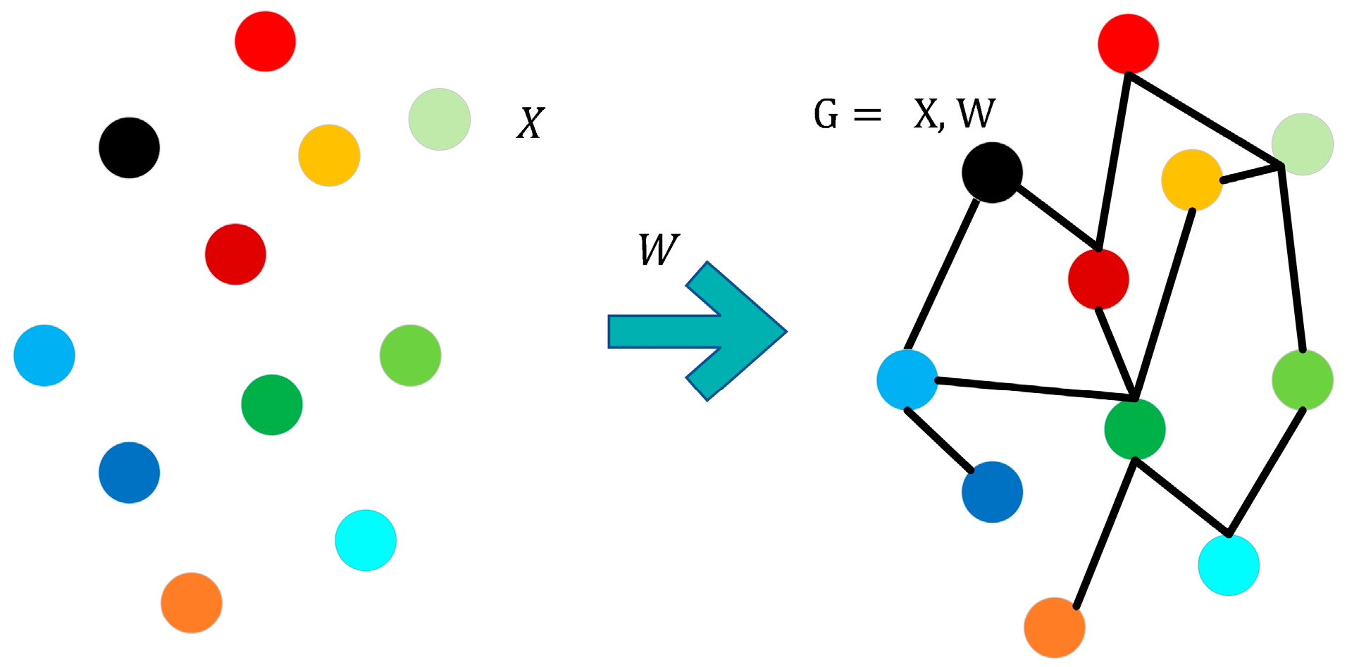
A new hybrid model PMNet is proposed in this paper. The PMNet has two branches. Among them, one is responsible for adaptive decomposition of PM2.5 signal and the other is used for extracting the correlation features of PM2.5 and other air pollutants. The overall framework of the PMNet is shown in Figure 1. The AVMD analyzes the characteristics of the target PM2.5 data, automatically determines the number of signal decomposition modes K and bandwidth constraint strength α, and then decomposes the PM2.5 data into a set of stable IMFs. The correlation extraction unit embedded in MtemGNN automatically extracts the correlation weight matrix W between multivariate time series X and constructs the correlation graph structure G = X , W to represent the correlation between PM2.5 and other air pollutants. The graph structure extracted by the embedded correlation unit is fed to the GCN unit, then transformed by the graph Fourier transform (GFT) into spectral domain for graph convolution feature extraction. The outputs of the two branches are integrated into one piece for GRU to learn the long-term and short-term dependence of the time series, thus obtaining the prediction results. The details of the structure and related method are provided in the subsequent sections.

2.2. AVMD

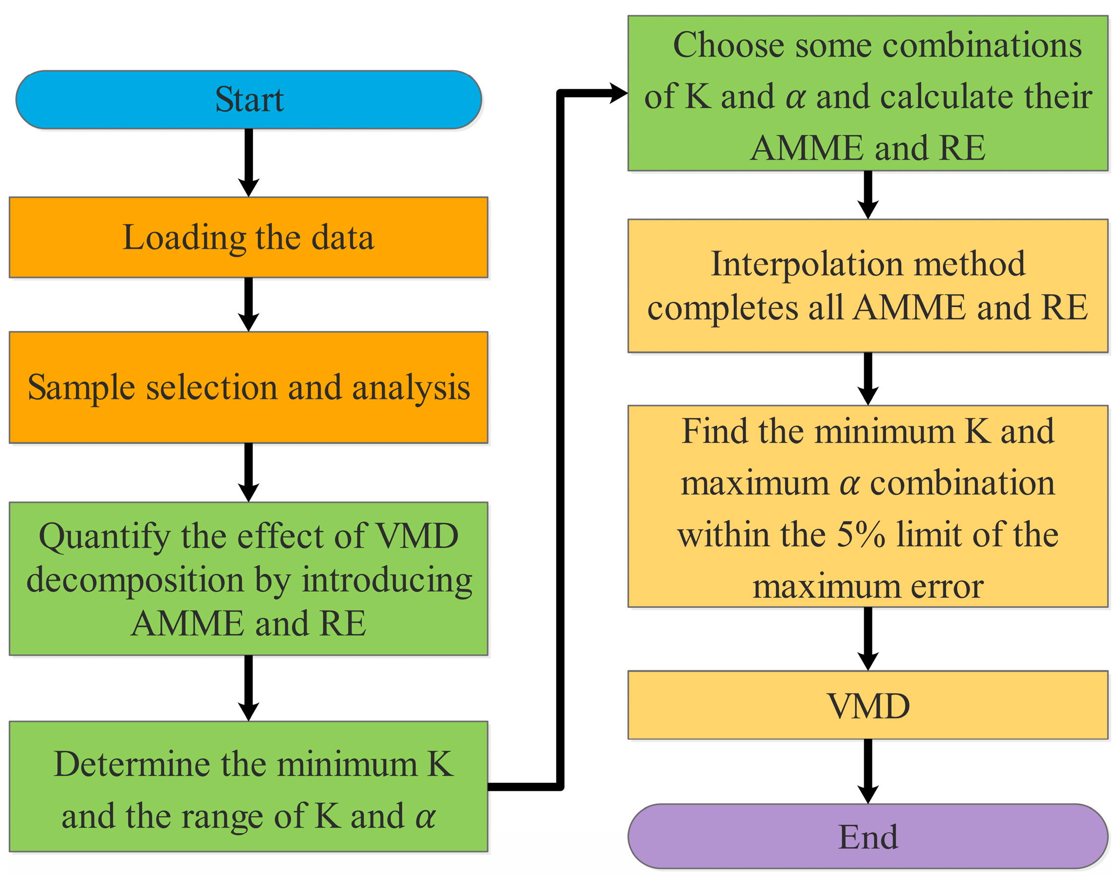
After setting the number of decomposition modes K and the central frequency bandwidth constraint α, VMD [34] decomposes the original non-stationary sequence into K IMFs, each confined in a specific bandwidth around its center frequency. The constraint degree α of the center frequency determines the bandwidth constraining degree of the IMF (please refer to Appendix A for a detailed description of VMD). The constraint strength α of center frequency bandwidth and the decomposition mode number K affect the quality of VMD decomposition considerably. When the value of K is fixed, a big value of bandwidth constraint degree α means that the decomposed modes will lose some information, which will make the sum of all decomposed modes deviate significantly from the real signal. The compensation method used to avoid large deviations is to increase the decomposition mode number K. However, further increasing K leads to over decomposition, which increases the accumulated error in model prediction, thus increasing the difficulty in improving the prediction accuracy of the model. When the value of α is small, although a small value of modal number K can be used, the phenomenon of mode mixing occurs, which is also not conducive to achieving high accuracy in model prediction. In order to solve the difficulty in selecting VMD decomposition parameters, this paper proposes a novel AVMD. The proposed AVMD automatically finds the optimal K-α combination on the basis of quantifying the VMD decomposition effect, and then decomposes the target data. The steps of AVMD decomposition are shown in Figure 2. The key steps include the quantization of VMD decomposition effect and the selection of optimal parameter combination. A detailed description is provided in the two subsequent sections.

2.2.1. Quantification of VMD Decomposition Effect

The reconstruction error (RE) should be considered first to quantify the VMD decomposition effect. In order to make the decomposed signal as close to the original signal as possible, the value of RE should not be too large. The RE is defined as follows:
R E = t = 1 N x ( t ) k = 1 K u k ( t )
where, u k is the k-th sub mode of decomposition, x t is value corresponding to the time t of the original time series, and N is the length of the decomposed time series.
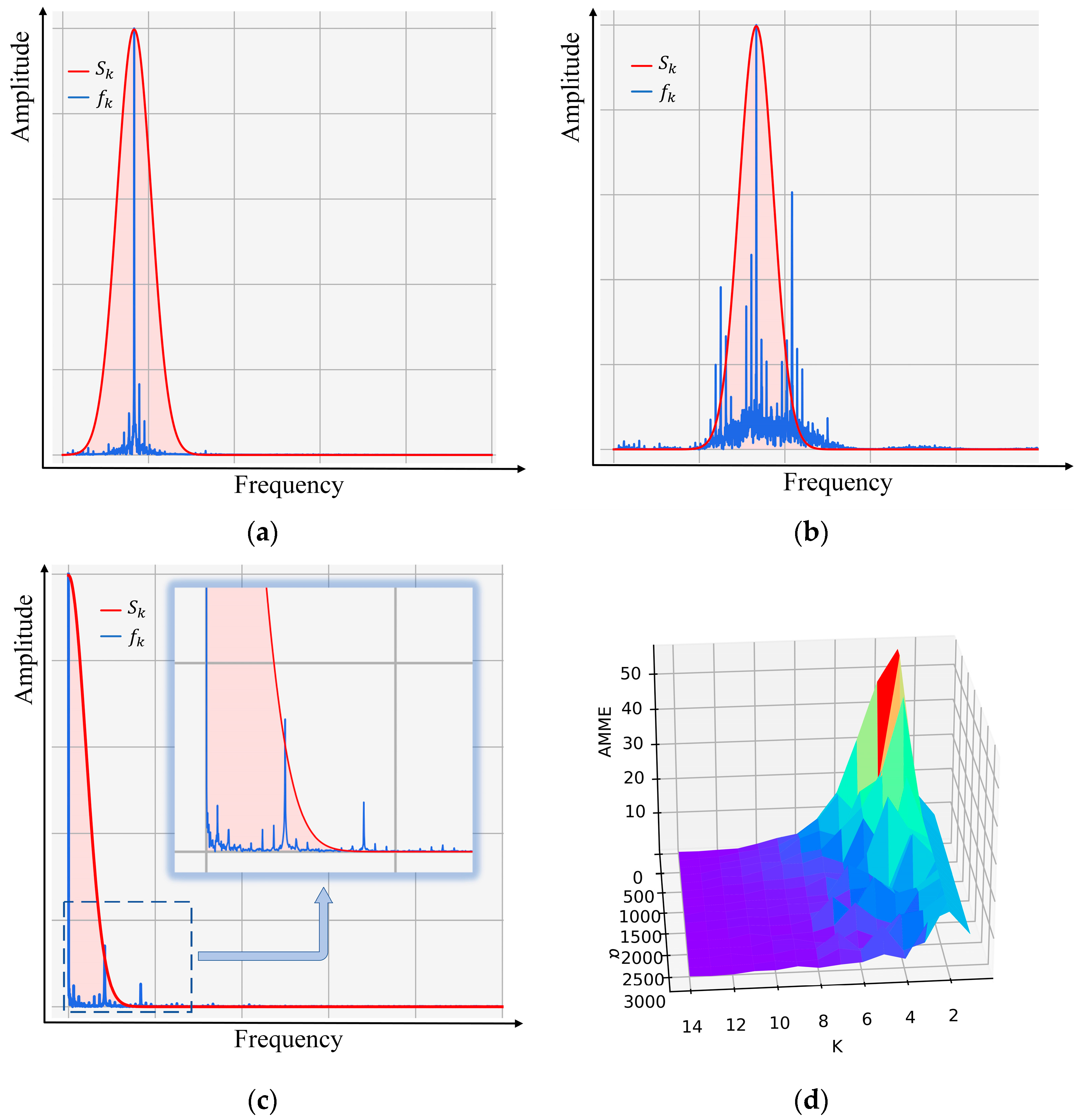
Increasing K or decreasing α continuously makes RE very small, but this may lead to over decomposition or mode mixing. Therefore, it is also necessary to find a metric to measure the degree of modal mixing in VMD decomposition and select the minimum value of K on the premise of ensuring acceptable degree of modal mixing and avoid over decomposition. As discussed, each IMF resulting from decomposition is confined within a specific bandwidth around its center frequency. The IMFs with severe mode mixing usually have more peaks and wider bandwidth, while IMFs with less severe mode mixing usually stay in a narrow bandwidth around the central frequency. Therefore, the spectrums of the IMFs with less severe mode mixing are better encompassed by a specific normally distributed probability density function, as shown in Figure 3a. On the other hand, the spectrums of the IMFs with severe mode mixing are more likely to dwell outside the specific normally distributed probability density function, as shown in Figure 3b.
In this paper, a normally distributed probability density function centering on the location of the central frequency of each IMF is constructed, and the degree of spectrum of IMF dwelling outside the normal distribution is used as the metric to analyze the degree of mode mixing. The relevant mathematical expressions are expressed as follows.
S k = 1 2 π σ exp ( ( m m k ) 2 2 σ 2 )
f k = Rescaling ( Γ ( u k ) )
e k ( m ) = f k ( m ) S k ( m ) , f k ( m ) S k ( m ) 0 0 , f k ( m ) S k ( m ) 0
A M M E = 1 K k = 1 K m = 1 M A k e k ( m ) d
where, S k represents the normally distributed probability density function corresponding to the k-th IMF,   m k represents the location of the center frequency of the k-th IMF, and m is the abscissa metric. For the convenience of normalizing the signal, the variance of the normally distributed probability density function is set to σ = 0.4 , which ensures that the highest point of the normal distribution is equal to that of the normalized IMF. f k   represents the spectrum of the k-th IMF after moralization, Rescaling represents min-max normalization, Γ u k represents the Fourier decomposition of u k , f k m represents the amplitude of the spectrum f k at location m of the frequency metric, and e k m   represents the error between f k m and S k (when the value of the f k m is greater than the S k m ). In order to effectively quantify mode mixing, the distance d between m and the x-axis coordinate of its IMF center frequency is defined to amplify the mode mixing of e k , which is far away from the center frequency. A k   represents the amplitude corresponding to the center frequency of the k-th IMF. The larger the value of A k , the larger is the proportion of the IMF spectrum in the total signal spectrum and more important is the IMF. Therefore, the spectra of IMFs with large A k are less tolerant to mode mixing. The average modal mixing error (AMME) efficiently reflects the severity of mode mixing in VMD. The smaller the value of AMME, the lower is the mode mixing degree in VMD decomposition and vice versa.

2.2.2. Selection of Optimal Parameter Combination

Please note that quantifying the VMD decomposition effect does not mean that the task of finding the optimal combination of decomposition mode number K and center frequency constraint strength α is accomplished. In order to find the K-α combination that yields the optimal VMD decomposition result, one complex and time-consuming method is to calculate the AMME and RE values for all possible parameter combinations. In principle, increasing the decomposition mode number K or decreasing the central frequency constraint strength α reduces the RS value. In addition, the rate of change diminishes continuously, and finally approaches saturation. Increasing the decomposition mode number K or the central frequency constraint strength α reduces the value of AMME, and the rate of change diminishes continuously and finally approach saturation. This phenomenon is similar to the effect of adjusting the filter size and network width in a neural network structure on the model accuracy and time consumption, i.e., the phenomena of supermodularity and submodularity [35]. Therefore, the problem of finding the appropriate K-α combination can be transformed into a submodular optimization problem or supermodular optimization problem. The definitions of supermodularity and submodularity are given in Appendix B.
Based on the supermodularity and submodularity, AMME and RE exhibit the change in K and α. This work selects a part of K-α combinations to compute the corresponding AMME and RE values. Then, the corresponding AMME and RE values are generated for all possible parameter combinations by interpolation and monotonization. Finally, find an appropriate K-α variety within the allowable error range. According to the variation characteristics of RE and AMME obtained by changing the values of K and α, the initial K-α combination should be as uniform as possible and the boundary values should be included. The excessively small values of K should be avoided as other frequency domain signals may be masked by large low-frequency components. When the value of K is too small, it leads to inconsistency between the decomposition result and the theoretical value. As shown in Figure 3c, when the selected value of K is low, most frequency domain signals are masked by low-frequency and large value components. Therefore, they cannot be decomposed and result in abnormal VMD decomposition. As shown in Figure 3d, an abrupt change in AMME occurs when the value of K is small. Therefore, the smallest value of K before abrupt change in AMME is regarded as the initial K.
According to some initial K-α combinations, the original data are decomposed by VMD to calculate the corresponding AMME and RE values, and then the inverse distance weighting interpolation [36] is used to fill the values of AMME and RE corresponding to all combinations within reasonable ranges. Due to the inherent submodularity and supermodularity in AMME and RE, the AMME and RE should show monotonicity with an increase in K or α. Please note that the real values obtained from the experiments are non-monotonic due to various uncertainties. Consequently, a monotonic correction function is required, which replaces the points that do not satisfy the monotonicity by correction values generated based on the monotonic interpolation. Increasing K and decreasing α continuously causes the RE and AMME to decrease monotonically and approach saturation, but over decomposition and excessively weak central frequency constraint may occur. In order to avoid over decomposition, AMME and RE should not be further reduced when the condition of the maximum error (5%) is satisfied. When the maximum allowable error (5%) is satisfied, the minimum value of K and the maximum value of α are selected to form the optimal parameter combination. Finally, the optimal parameter combination is fed to the VMD module to complete signal decomposition.

2.3. MtemGNN

The graph neural network (GNN) that is a relatively new neural network, is a fusion of graph structure and traditional neural network [37]. The introduction of graph structure breaks the traditional representation of Euclidean distance and effectively represents the intrinsic correlation between different objects. MtemGNN uses the graph structure in GNN to represent the correlation characteristics of multivariate time series and is inspired by StemGNN, which is a multivariate time series prediction method [28].
In this study, the spectral sequential cell responsible for learning the frequency characteristics of a single time series in StemGNN is omitted in MtemGNN. There are two reasons for this omission. First, the cell can only learn very limited time series information, which is very inefficient as compared with AVMD’s ability of learning overall frequency characteristics of a time series. More importantly, the frequency of short-term time series is usually unstable, so the cell is not helpful for the extraction of time series features. MtemGNN consists of a latent correlation layer and a GCN layer. As GNN needs a graph structure to construct the correlation representation of multivariate time series, the latent correlation layer is needed to automatically infer the correlation graph representation of multivariate time series. The GCN layer is used to extract the features from a graph structure.

2.3.1. Latent Correlation Layer

For some specific structures, it is feasible to determine the graph structure between them based on the prior knowledge, such as road network in traffic prediction. However, in most circumstances, no prior knowledge is available for constructing the graph structure. Therefore, the self-attention mechanism [38] is used to automatically learn the intrinsic correlation graph structure of multivariate time series. Specifically, the self-attention mechanism automatically calculates the correlation between each time series with all other time series to obtain the correlation representation of the former. The multivariate time series X is sent to the GRU to iteratively update the state of the hidden layer. The state of the last hidden layer R is used to represent the entire time series. Afterwards, the correlation between the time series is calculated by using the self-attention mechanism. The formula for calculating self-attention correlation weight matrix is:
Q = R W Q , Κ = R W Κ , W = Softmax ( Q Κ T d )
where, Q   and K represent “query” and “key”, respectively, which are calculated using the linear projections of the learnable parameters W Q and W K in the attention mechanism. d is the number of hidden dimensions in Q   and K. The adjacent matrix of graph G , W N × N represents the correlation between the time series. The graph structure is represented by correlation weight matrix and multivariate time series, as shown in Figure 4.

2.3.2. GCN Layer

As shown in Figure 1, the GCN layer consists of two stacked GCN blocks [39]. The residual connection mechanism is used to connect two GCN blocks for obtaining a deeper model [40]. Specifically, the second GCN block attempts to construct the residual between the real value and the reconstructed value of the first GCN block. Each block has two branches, i.e., the forecasting branch for predicting future values and the backcasting branch for reconstructing the historical values. The backcasting branch helps to learn the residual representation and adjust the structure of the prediction model. As the number of edges connected to each node in the graph structure varies from node to node, it is impossible to perform convolution with a fixed convolution kernel. One classic and efficient graph convolution method is to first convert the spatial domain data to spectral domain based on GFT and then perform convolution GConv in spectral domain, and finally convert the data back to the spatial domain through inverse graph Fourier transform (IGFT).
Similar to the traditional Fourier transform, the GFT [41] finds a set of orthogonal bases and decomposes the graph based on these orthogonal bases for representation. The process of decomposing the eigenvalues of Laplacian matrix in the graph is the process of finding the orthogonal bases needed to construct the graph. The normalized Laplace matrix [42] is expressed as L s y m = I N D 1 2 W D 1 2 , where I N N × N is the unit matrix and D is a diagonal matrix whose diagonal values represent the number of edges connected with each node. The eigenvalues of Laplace matrix are decomposed into L = U Λ U T , where U N × N   is the eigenvector of the matrix and Λ is the diagonal matrix of eigenvalues. For a given multivariate time series X N × T , GFT, GConv, and IGFT are defined as G F X = U T X = X ^ ,   GConv X ^ = σ L s y m X ^ W l ,   and G F 1 GConv X ^ = U GConv X ^ , respectively, where W l is the learnable parameter matrix and σ is the activation function.

2.4. GRU

The GRU [43] is a variant of the relatively new recurrent neural network and solves the problems of gradient disappearance and gradient explosion during RNN training. The GRU has a learning ability similar to LSTM, but its internal structure is simpler, which means that a smaller number of calculations are required [44].
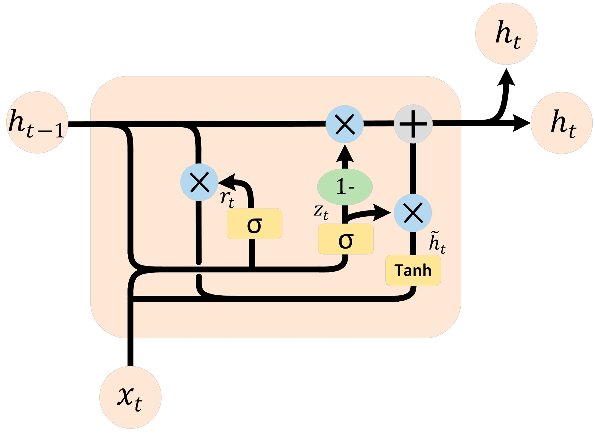
The GRU is composed of an update gate, a reset gate, and an output gate, capable of effectively extracting the long-term and short-term features from a time series [45]. The architecture of GRU is presented in Appendix C.
The update gate has the functions of forgetting and selective memory, which is equivalent to the combination of LSTM input gate and forgetting gate. The calculation formula of the update gate is shown in Equation (7), where z t represents the update gate, which is used to control the extent to which the state information of the previous time is used in the current state. The larger the value of the update gate, more information from the previous state is used. h t 1 represents the output vector of previous time and x t represents the input vector of current time.
z t = σ ( w z 1 h t 1 + w z 2 x t + b )
The calculation process of the reset door is shown in Equation (8), where r t represents the reset gate, which is used to control the amount of information from the previous time used by the candidate information of the current time.
r t = σ ( w r 1 h t 1 + w r 2 x t + b r )
The reserved information h ˜ t at the current time is updated as:
h ˜ t = tanh ( w h 1 r t h t 1 + w h 2 x t + b h )
Considering the retention vector h ˜ t and the output vector after updating the output gate, the output vector h t obtained at the current time is expressed as:
h t = ( 1 z t ) h t 1 + z t h ˜ t
where, w z 2 ,     w r 2 ,   and   w h 2 represent the weight of input x t in each operation. w z 1 ,     w r 1 ,   and   w h 1   represent the weight of output h t in each operation.

3. Experimental Results

3.1. Settings

The deep learning models used in this paper are developed using Python. The experimental environment includes 64-bit Windows 10 operating system, Intel Core i5-10500H processor, and main frequency 2.5 GHz. All the experiments in this work are conducted under the same conditions.
The dataset used in our experiment is acquired during the period from 1 January 2018, to 31 December 2021, in Beijing. The sampling interval was 1 h, i.e., 24 samples were taken every day. The monitoring dataset is released by China Environmental Monitoring Station on https://air.cnemc.cn:18007/ (accessed on 18 September 2022). The average value of all sites was used as the Beijing PM2.5 data in this experiment to prevent a large number of missing data due to the selection of single-site data. The dataset includes the concentrations of AQI, PM2.5, PM10, SO2, NO2, O3, CO, and the average concentration of these pollutants during the prior 8 h and the prior 24 h.
The experimental data are divided into three parts, i.e., 70% of the information is used as a training set, 20% as a verification set, and 10% as the test set. It can be seen from the data in Table 1 that the data of the last 24 h is used as input to predict the PM2.5 during the next 12 h. The initial learning rate, epochs, and batch size are 0.001, 150, and 24, respectively. MSE loss and RMS Prop are used as loss functions and optimizers, respectively.

3.2. AVMD Performance

In the AVMD experiment, a set of PM2.5 data acquired during 4000 consecutive hours is used as an input of AVMD to estimate the best K-α combination. For the convenience of observation, each IMF spectrum’s ordinate and abscissa metrics are normalized. To effectively distinguish the mode mixing, the abscissa scale of the customarily distributed probability density function is shrunken by ten times based on the experimental data. By analyzing the data of PM2.5, power load, and electricity price, and by consulting the relevant published papers in the field of AVMD, it is determined that the reasonable range of α is (100, 3100) and the upper limit of K is (16).
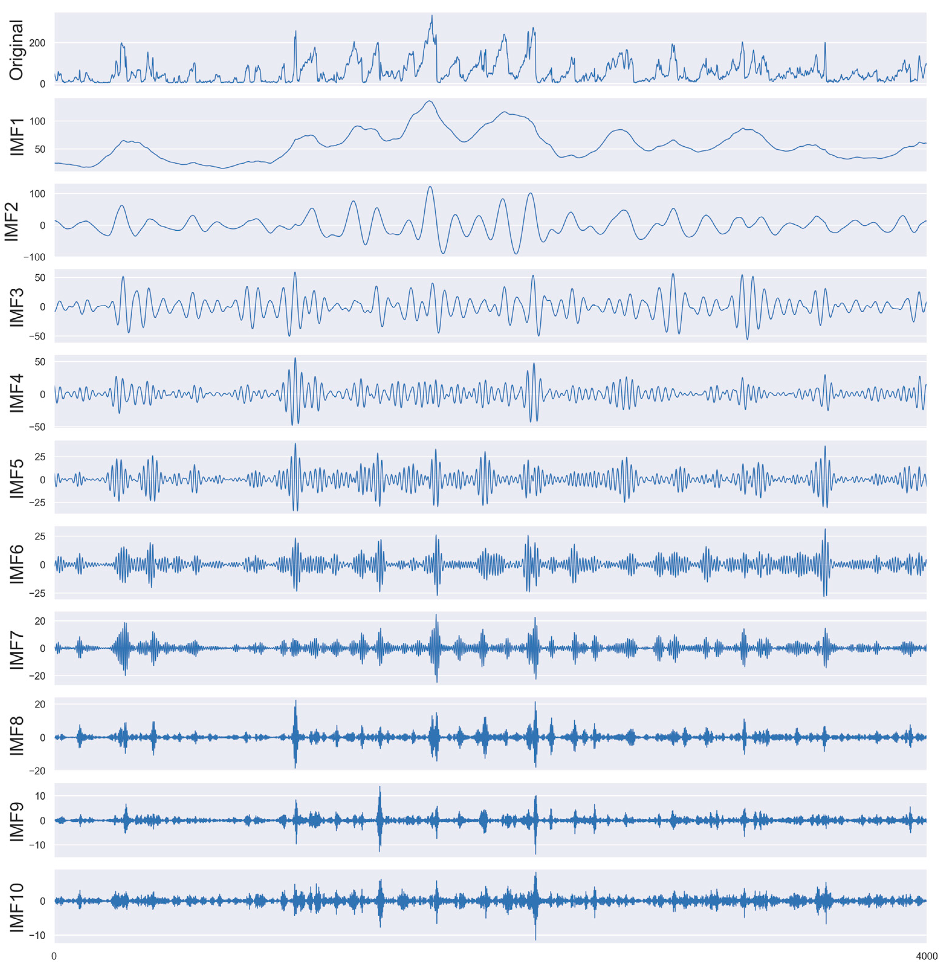
AVMD automatically decomposes the PM2.5 data of Beijing into 10 IMFs with a center frequency bandwidth constraint strength of 1000. The local curves of the original signal and the decomposed IMFs were drawn to observe the stationarity of the IMFs after AVMD decomposition. As shown in Figure 5, the low-frequency signals IMF1 and IMF2 determine the general direction of the original signal, which is more stable than the original signal, helping the model extract the features of the low-frequency signal. The internal signal frequencies of the remaining IMFs are fixed in a particular frequency band, respectively, which is convenient for model feature extraction.
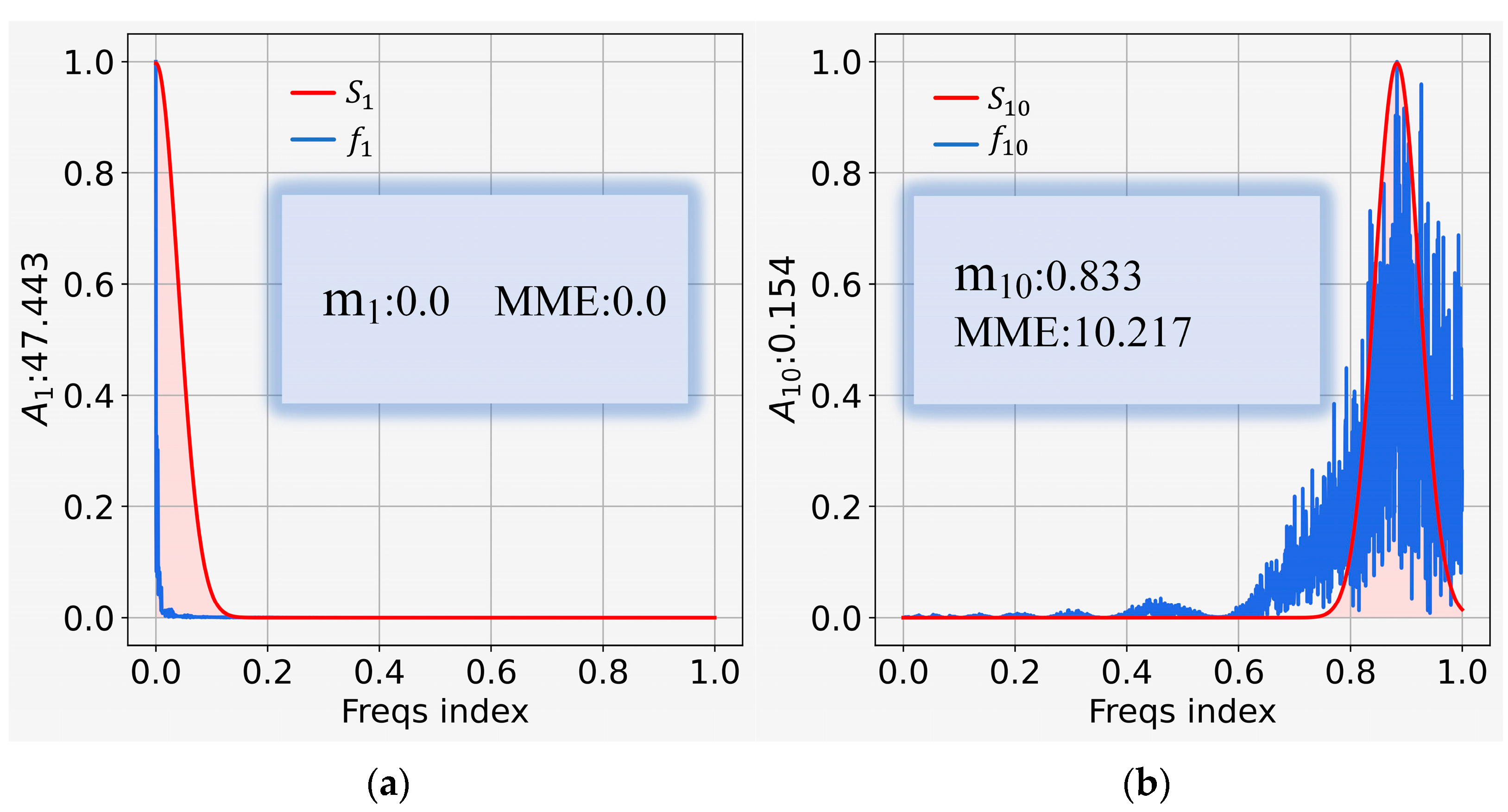
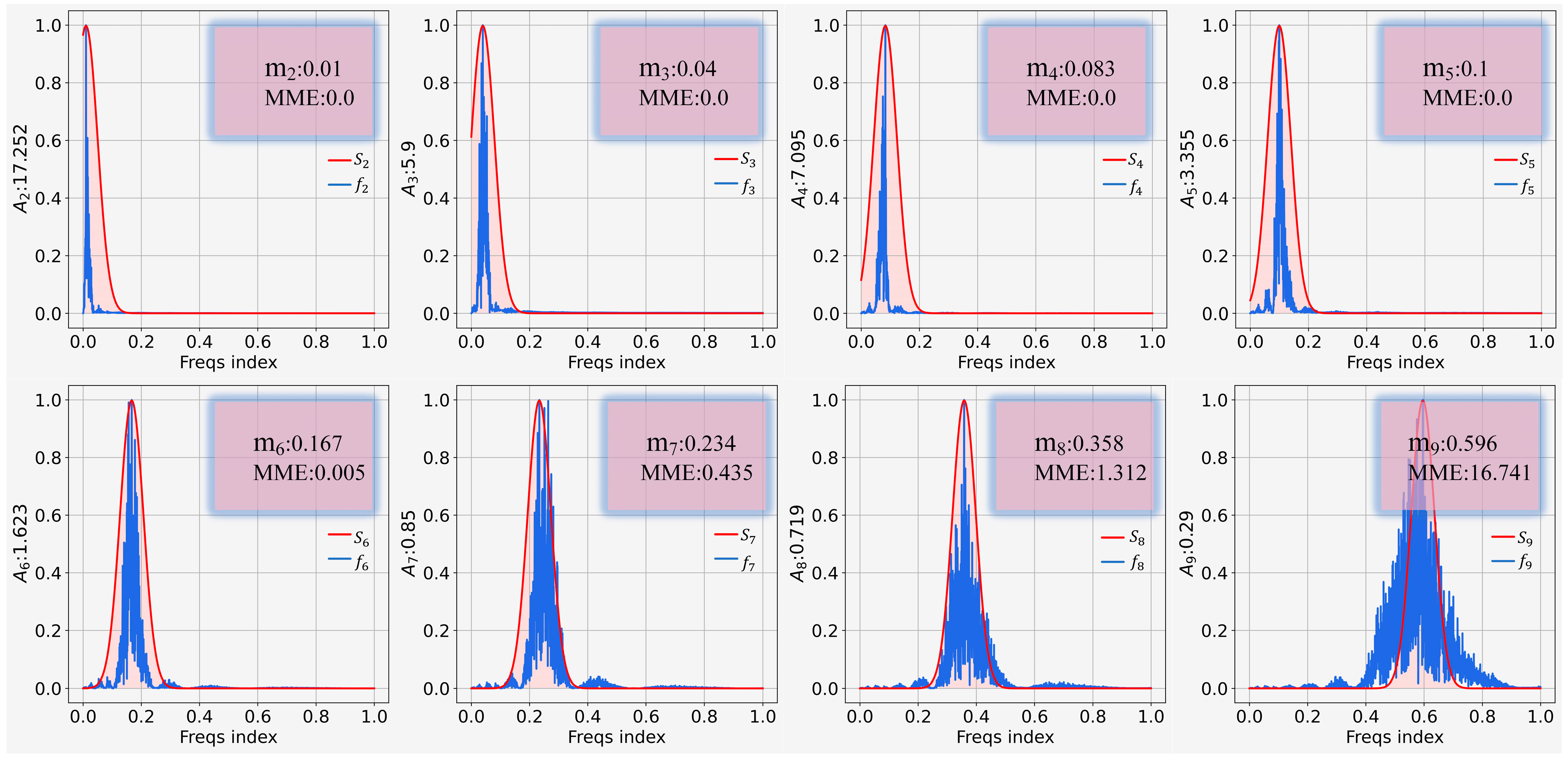
The visualized mode mixing degrees of two typical IMFs are shown in Figure 6. Where A1 and A10 represent the amplitudes of the center frequencies of IMF1 and IMF10, respectively, m1 and m10 represent the indices of the normalized center frequencies, and MME represents the degree of mode mixing of IMFs. The center frequency index in Figure 6a is 0, and the center frequency index in Figure 6b is close to 1. The center frequency indices of the remaining IMFs in Appendix D are scattered between 0 and 1, which verifies that the IMFs obtained by AVMD decomposition have obvious internal frequency characteristics and are easy to extract. As shown in Figure 6a, the spectrum with a larger amplitude value A1 cannot tolerate larger modal mixing, so our AVMD algorithm can better constrain the spectrum within the probability density function of the normal distribution. As shown in Figure 6b, the spectrum with small amplitude values A10 can tolerate a certain degree of mode mixing, thus the over decomposition as a result of pursuing low mode mixing degree can be avoided.
The visualization of two typical cases of mode mixing with different degrees proves that the proposed AVMD not only effectively reduces the phenomenon of mode mixing, but also avoids over decomposition. An existing AVMD quickly finds the value of K automatically by adding a decomposition quality evaluation criterion. However, it ignores the central frequency bandwidth constraint of real α and over decomposition. As a result, the value of K continuously increases in pursuit of low mode mixing degree [46]. Few AVMDs use the prior knowledge obtained from data analysis to fix the value of K and introduce the mode mixing degree evaluation metric to find an appropriate value of α. This type of AVMD is only suitable for processing the data of some specific types and is not universally applicable [47]. The AVMD proposed in this paper is based on sample data analysis instead of prior knowledge. Therefore, it can be automatically and flexibly applied to different types of data.

3.3. Performance Evaluation Indices

In this paper, MAPE, MAE, and RMSE are used as performance evaluation metrics to evaluate the prediction accuracy of the model. These metrics are mathematically expressed as:
M A P E = 1 n i = 1 n y ˜ i y i y i × 100 %
M A E = 1 n i = 1 n y ˜ i y i
R M S E = 1 n i = 1 n y ˜ i y i 2
where, y i ˜ is the i -th prediction value and y i is the i -th real value. It can be seen from the above formulas that the MAE calculates the difference between the predicted value and the real value, and then takes the average value of the sum of absolute values. n is the length of the time series.
Please note that the learning rate affects the experimental results. If the value of learning rate is too large, the neural network does not converge. If the value of learning rate is too small, the neural network is likely to fall into a local minima. In order to avoid the unstable factors caused by improper setting of learning rate, all the tests in the experiment use dynamic learning rate, with the batch size set to 24 and epochs set to 150. The initial value of learning rate is set to 0.0007 and is attenuated by 0.5 times after every 40 epochs.

3.4. Comparison of the PMNet with Other Prediction Methods

Considering their good performance in the previous PM2.5 prediction, LSTM and GRU are used as baseline models to compare with PMNet. In addition, the multivariate time series prediction model StemGNN is also compared. Considering that the multi-step PM2.5 prediction is challenging for the baseline models, the prediction results with a time step of 3 h are chosen for comparison (see Table 2).
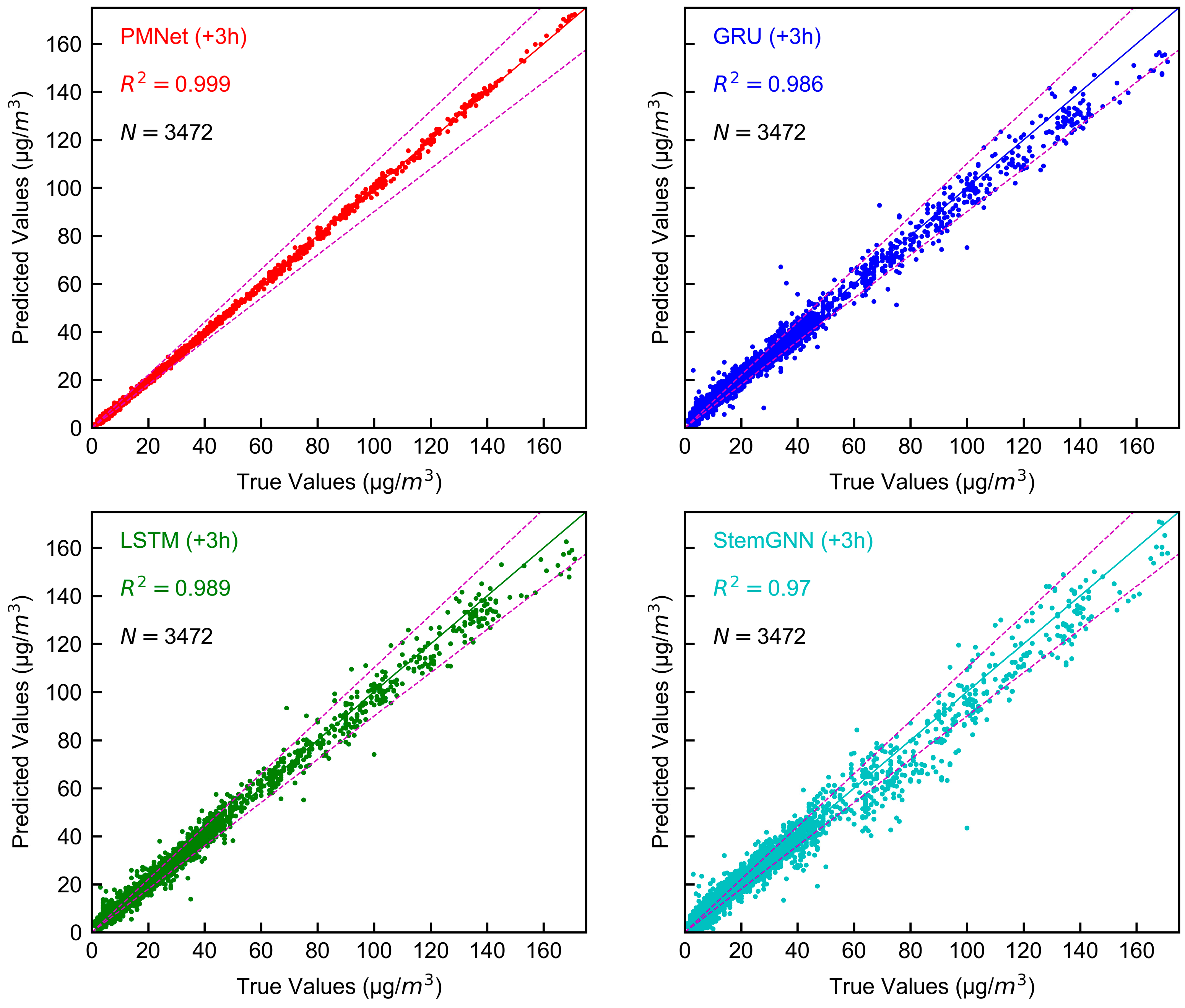
As compared with other models, the PMNet achieves the best performance in terms of all evaluation metrics in the test of 3-h PM2.5 prediction. It is worth noting that the performance of PMNet does not decrease significantly with an increase in time step, and the baseline models exhibit poor performance in multi-step prediction. The value of PM2.5 is comparatively tiny compared to fluctuations, making the value of MAPE more sensitive. The partial real value tracking curves can be seen in Figure 7. The curve predicted by PMNet most of the time follows the natural value curve. LSTM and GRU can track the approximate direction of the actual value but have lower prediction accuracy. The result predicted by StemGNN is considerably different from the real value curve and has the most insufficient confidence. The scatter plot containing the forecast effect at all times of the test data is shown in Figure 8. R2 represents the correlation coefficient between the actual values and the predicted values, and the larger the R2 value, the smaller the error between the predicted values and the actual values. PMNet predicted, and truth values are always clustered around the diagonal, indicating the lowest prediction error and the best prediction performance. LSTM and GRU have a certain discreteness when predicted values are significant, but most scattered points fall within the purple dotted lines on both sides of the MAPE of 10%. Many scatter points in the StemGNN prediction are beyond the dashed lines on both sides of the MAPE of 10%, which has the lowest reference value in the 3-h PM2.5 forecast.

3.5. Ablation Experiment

To better understand the effectiveness of different components in the PMNet, three incomplete versions of the PMNet are designed to compare with the complete PMNet.
The incomplete and complete models are used to perform 12-h P2.5 prediction test. The average errors of the models are calculated and compared. The results are shown in Table 3.
w/o MtemGNN: The MtemGNN module is removed from the PMNet to observe its impact. The Table 3 shows that the addition of the MtemGNN module in the PM2.5 prediction model reduces MAPE, MAE, and RMSE by 38.30%, 40.556%, and 39.282%, respectively. The experimental results show that MtemGNN extracts the correlation features between PM2.5 and other air pollutants efficiently, which greatly improves the accuracy of the model.
w/o GRU: The GRU module is removed from the PMNet to observe its impact. The Table 3 shows that the addition of the GRU module in the PM2.5 prediction model reduces the MAPE, MAE, and RMSE by 71.76%, 73.674%, and 72.624%, respectively. The experimental results show that the GRU learns the long-term time dependence of time series efficiently. Therefore, it significantly improves the accuracy of PM2.5 prediction, which demonstrates that the GRU is an indispensable part of an accurate PM2.5 prediction model.
w/o AVMD: The AVMD module is removed from the PMNet to observe its impact. The Table 3 shows that the addition of the AVMD module in the PM2.5 prediction model reduces MAPE, MAE, and RMSE by 88.093%, 90.141%, and 91.691%, respectively. The experimental results show that the addition of AVMD results into a dramatic improvement in the performance of the PM2.5 prediction model, which can be attributed to the ability of AVMD to transform non-stationary time series into a series of stable IMFs. These IMFs have prominent frequency characteristics and represent the spectral characteristics of time series PM2.5 data, which is of great help to PM2.5 prediction model.
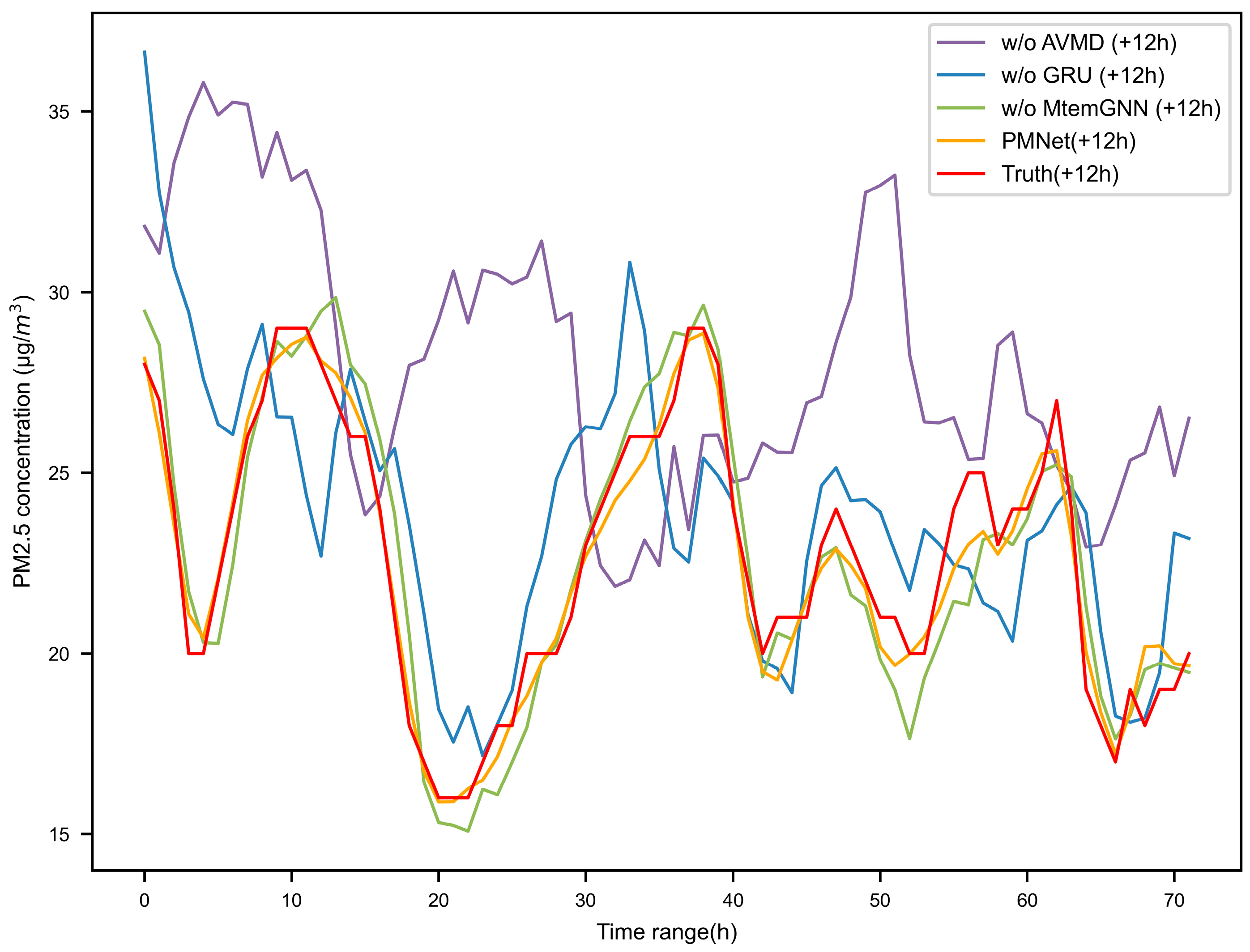
Figure 9 depicts partial (72 h) real value tracking curves of the ablation experiment. Even if PM2.5 is predicted for the 12th hour in the future, the PMNet prediction curve still closely follows the actual value curve, which indicates that the PMNet still has a reliable prediction effect in the PM2.5 prediction at the 12th hour. In general, the model without MtemGNN also has a good prediction effect. However, the prediction performance at the peaks and troughs is still lacking, which reveals that adding MtemGNN significantly improves multi-step prediction. w/o GRU and w/o AVMD did not perform well, highlighting the importance of AVMD and GRU for half-day PM2.5 prediction.
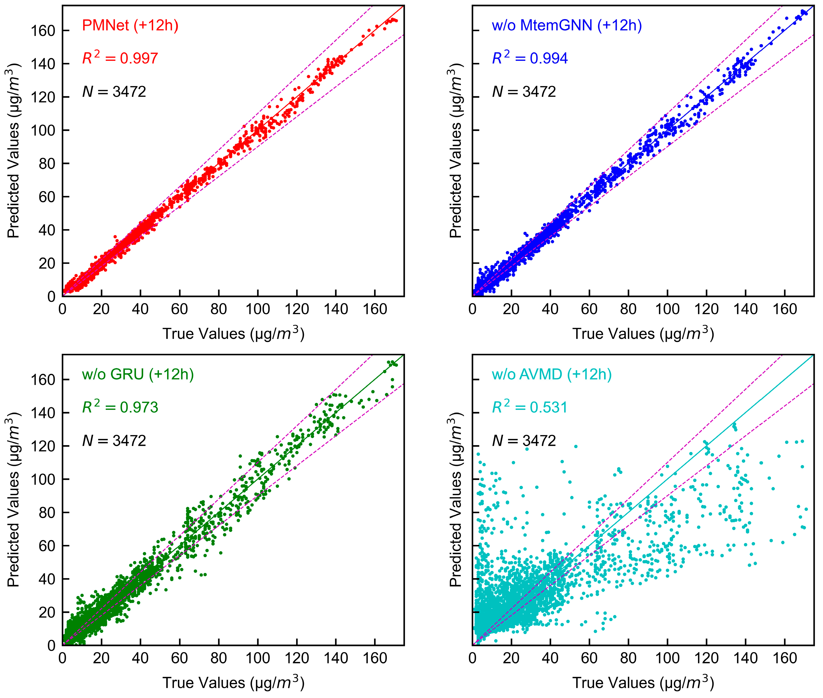
The distribution of all the actual values and the predicted values in the ablation experiment can be further displayed from the scatter plot in Figure 10. Compared with PMNet, w/o MtemGNN has a more significant dispersion of scattered points, which means that the correlation between the predicted and actual values is slightly worse. The prediction effect of w/o GRU is worse than that of w/o MtemGNN, which reveals that the long-term memory properties of time series are more important than the correlation among multivariate time series. The predicted values of w/o AVMD are so different from actual values that the prediction of PM2.5 at 12 h is no longer reliable. This demonstrates that AVMD contributes the most to the model, followed by GRU and MtemGNN last.

4. Discussion

This paper verifies the effect of the PM2.5 prediction model combining AVMD and MtemGNN from multiple perspectives. First, the decomposition development is analyzed by visualizing the sequence and spectra of IMFs in Figure 5 and Figure 6. The proposed AVMD effectively reduces the mode mixing problem while avoiding over-decomposition. This result may be explained by the fact that AVMD considers reconstruction error and mode mixing error to improve the quality of IMFs while choosing the smallest K. Secondly, according to Table 2, Figure 7 and Figure 8, comparing the prediction effects of PMNet and the baseline model, PMNet is the most stable and accurate in multi-step PM2.5 prediction. It is illustrated that AVMD and MtemGNN in the PMNet model have improved the PM2.5 prediction accuracy. Finally, the effect of each component inside PMNet is analyzed through ablation experiments. Finally, the impact of each element inside PMNet is analyzed through ablation experiments. Table 3 presents that AVMD is the most important, followed by GRU and MtemGNN. This result implies that the PM2.5 smoothing process is the first factor that should be considered in PM2.5 prediction, and the long-term and short-term memory characteristics of time series are also required. Adding MtemGNN reduces RMSE by 39.282%, which is still very helpful for improving the accuracy of multi-step PM2.5 prediction.
To discuss the contributions of this paper more broadly, other studies in related fields are described in Table 4. To be sure, all the studies made some progress. A note of caution is due here since the RMSE of Huang et al. is much higher than others in the list, which may be due to the use of the Beijing Capital Airport dataset with large and volatile data values. The RMSE of Yang et al. is the lowest in the list but still slightly worse than the RMSE = 0.731 predicted by PMNet at 1 h. An interesting finding is that the decomposition algorithm was used to stabilize PM2.5 in three studies, which again illustrates the importance of PM2.5 stabilization and the guiding role of AVMD for subsequent analyses. Another important finding is that six studies used variants of recurrent neural networks (LSTM, GRU, biLSTM), which indicates that it is universally adaptable to extract long- and short-term time-dependent features in PM2.5 predictions. Several studies proposed using multiple input variables to predict PM2.5 but did not consider the correlation feature extraction between multivariate inputs that have been proven effective in PMNet. In future research, combining the spatiotemporal relationship to improve PMNet may be an important research direction.

5. Conclusions

This paper proposes a novel PM2.5 prediction model by combining AVMD and MtemGNN, named PMNet. PMNet obtained outstanding results on a real dataset acquired in Beijing. The AVMD not only effectively mitigates the mode mixing, but also avoids the occurrence of over decomposition and effectively solves the difficulty of parameter selection in VMD. The target PM2.5 data are automatically decomposed into a series of stable IMFs by AVMD. Each IMF has prominent frequency domain characteristics. As a result, it is easy to extract the intrinsic features from PM2.5 time series and significantly improve the accuracy of PM2.5 prediction. The addition of GNN provides a fresh idea for presenting the correlation between PM2.5 and other air pollutants, as well as for extracting features from a time series. The results of ablation experiments demonstrate that the addition of MtemGNN to the PM2.5 prediction model significantly improves the prediction accuracy, which proves the effectiveness of MtemGNN. In addition, the use of GRU provides the capability of learning the long-term and short-term characteristics of the time series processed by AVMD and MtemGNN, which further improves the performance of the PMNet. As compared with the baseline models, the proposed hybrid model achieves much better performance in terms of all three-evaluation metrics. The PMNet also achieves very high accuracy in predicting PM2.5 concentration for the next 12 h. This information is used to provide the guidance for ordinary people to take the protective measures and helps the government to control air pollution. All parts of the proposed PM2.5 hybrid prediction model are data-driven, which means that the PMNet can be flexibly applied to PM2.5 prediction in other regions. In future research, multi-task learning will be introduced into PMNet to incorporate the Spatio-temporal correlation and enable PMNet to predict PM2.5 concentrations in multiple regions simultaneously.

Author Contributions

Conceptualization: Y.P.; Data curation: Y.P.; Formal analysis: Y.P.; Funding acquisition: Y.P.; Investigation: C.-J.H.; Methodology: Y.P. and C.-J.H.; Project administration: Y.P., C.-J.H.; Resources: C.-J.H.; Software: C.-J.H., Y.P., Y.S. and Y.M.; Supervision: C.-J.H.; Validation: C.-J.H., Y.P., Y.S., and Y.M.; Visualization: C.-J.H. and Y.P.; Writing—original draft: C.-J.H. and Y.P.; Writing—review and editing: C.-J.H. and Y.P. All authors have read and agreed to the published version of the manuscript.

Funding

This research was funded by Youth Project of Chongqing, grant number: KJQN202202402.

Institutional Review Board Statement

Not applicable.

Informed Consent Statement

Not applicable.

Data Availability Statement

The data is obtained from https://air.cnemc.cn:18007/ (accessed on 18 September 2022).

Conflicts of Interest

The authors declare no conflict of interest.

Appendix A. VMD

VMD is a novel and theoretically sound non-recursive signal decomposition algorithm proposed by Dragomiretskiy and Zosso in 2014 [34]. Contrary to the traditional wavelet decomposition and EMD, VMD uses Wiener filter as the narrowband priori in frequency domain to constrain the decomposed sub-modes in the specific bandwidth around the central frequency, thereby effectively avoiding the mode mixing in signal decomposition. The working principle of VMD is to decompose the original signal into K IMFs, with each IMF being confined within a specific bandwidth around the center frequency.
The idea of constraining the IMF within the bandwidth around the center frequency originates from Wiener filtering, which performs Hilbert transform [54] on each sub-signal u k to obtain the corresponding analytical signal f A .
f A = ( δ ( t ) + j π t ) u k ( t )
Each analytic signal is mixed with the exponential term   e j ω k t for modulating the sub signal spectrum with the baseband. Then, the bandwidth is represented by the Gaussian smoothness. The variational constraint problem is represented by the following expression:
min u k , ω k k t ( δ ( t ) + j π t ) u k ( t ) e j ω k t 2 2
s . t . k u k = f
where, u k   and   ω k represent the set of all modes u k and the set of all center frequencies ω k , respectively.
In order to easily estimate the sub-signal u k and center frequency   ω k , this work uses the augmented Lagrange L to transform the original variational constraint problem into an unconstrained variational problem:
L u k , ω k , λ = α k t δ ( t ) + j π t u k ( t ) e j ω k t 2 2 + λ t , f ( t ) k u k ( t ) + f ( t ) k u k ( t ) 2 2
The augmented Lagrangian saddle point is solved using the alternate direction method of multipliers [55], on the basis of which the sub-signal u k and center frequency ω k are solved.
ω k   is treated as a constant. Thus, the problem of updating u k is transformed into a minimization problem as expressed below:
u k n + 1 = arg min u k X α t δ ( t ) + j π t u k ( t ) e j ω k t 2 2 + f ( t ) k u k ( t ) + λ ( t ) 2 2 2
u k is treated as a constant, thus the problem of updating ω k is also transformed into a minimization problem as expressed below:
ω k n + 1 = arg min ω k t δ ( t ) + j π t u k ( t ) e j ω k t 2 2

Appendix B. Submodularity and Supermodularity

The submodularity and supermodularity are properties of set functions. The submodular function monotonically increases with an increase in the number of set elements. Its second derivative is greater than or equal to zero and approaches saturation with an increase in the number of set elements. The supermodular function is the converse of submodular function. The definitions of these two types of functions are as follows:
Given a set function f :   2 V , if it satisfies A⊆B⊆V, and for all   s V \ B , it satisfies:
f A s f A f ( B s ) f B
then, set function f is a submodular function.

Appendix C. The Architecture of GRU

Sustainability 14 13191 i001

Appendix D. Visualization of Mode Mixing for the Remaining IMFs
Sustainability 14 13191 i002

References

  1. WHO. Available online: https://www.who.int/health-topics/air-pollution#tab=tab_1 (accessed on 18 September 2022).
  2. Meo, S.A.; Almutairi, F.J.; Abukhalaf, A.A.; Alessa, O.M.; Al-Khlaiwi, T.; Meo, A.S. Sandstorm and its effect on particulate matter PM 2.5, carbon monoxide, nitrogen dioxide, ozone pollutants and SARS-CoV-2 cases and deaths. Sci. Total Environ. 2021, 795, 148764. [Google Scholar] [CrossRef] [PubMed]
  3. Yang, B.-Y.; Qian, Z.M.; Li, S.; Fan, S.; Chen, G.; Syberg, K.M.; Xian, H.; Wang, S.-Q.; Ma, H.; Chen, D.-H.; et al. Long-term exposure to ambient air pollution (including PM1) and metabolic syndrome: The 33 Communities Chinese Health Study (33CCHS). Environ. Res. 2018, 164, 204–211. [Google Scholar] [CrossRef] [PubMed]
  4. Schneider, R.; Vicedo-Cabrera, A.; Sera, F.; Masselot, P.; Stafoggia, M.; de Hoogh, K.; Kloog, I.; Reis, S.; Vieno, M.; Gasparrini, A. A Satellite-Based Spatio-Temporal Machine Learning Model to Reconstruct Daily PM2.5 Concentrations across Great Britain. Remote Sens. 2020, 12, 3803. [Google Scholar] [CrossRef]
  5. Guo, H.; Li, W.; Wu, J. Ambient PM2.5 and Annual Lung Cancer Incidence: A Nationwide Study in 295 Chinese Counties. Int. J. Environ. Res. Public Health 2020, 17, 1481. [Google Scholar] [CrossRef] [Green Version]
  6. Aldegunde, J.A.Á.; Sánchez, A.F.; Saba, M.; Bolaños, E.Q.; Caraballo, L.R. Spatiotemporal Analysis of PM2.5 Concentrations on the Incidence of Childhood Asthma in Developing Countries: Case Study of Cartagena de Indias, Colombia. Atmosphere 2022, 13, 1383. [Google Scholar] [CrossRef]
  7. Cao, X.; Shen, L.; Wu, S.; Yan, C.; Zhou, Y.; Xiong, G.; Wang, Y.; Liu, Y.; Liu, B.; Tang, X.; et al. Urban fine particulate matter exposure causes male reproductive injury through destroying blood-testis barrier (BTB) integrity. Toxicol. Lett. 2017, 266, 1–12. [Google Scholar] [CrossRef]
  8. Wei, Y.; Cao, X.-N.; Tang, X.-L.; Shen, L.-J.; Lin, T.; He, D.-W.; Wu, S.-D.; Wei, G.-H. Urban fine particulate matter (PM2.5) exposure destroys blood–testis barrier (BTB) integrity through excessive ROS-mediated autophagy. Toxicol. Mech. Methods 2018, 28, 302–319. [Google Scholar] [CrossRef]
  9. Coccia, M. How do low wind speeds and high levels of air pollution support the spread of COVID-19? Atmos. Pollut. Res. 2021, 12, 437–445. [Google Scholar] [CrossRef]
  10. Namdar-Khojasteh, D.; Yeghaneh, B.; Maher, A.; Namdar-Khojasteh, F.; Tu, J. Assessment of the relationship between exposure to air pollutants and COVID-19 pandemic in Tehran city, Iran. Atmos. Pollut. Res. 2022, 13, 101474. [Google Scholar] [CrossRef]
  11. van Beest, M.R.R.S.; Arpino, F.; Hlinka, O.; Sauret, E.; van Beest, N.R.T.P.; Humphries, R.S.; Buonanno, G.; Morawska, L.; Governatori, G.; Motta, N. Influence of indoor airflow on particle spread of a single breath and cough in enclosures: Does opening a window really ‘help’? Atmos. Pollut. Res. 2022, 13, 101473. [Google Scholar] [CrossRef]
  12. Setti, L.; Passarini, F.; De Gennaro, G.; Barbieri, P.; Perrone, M.G.; Borelli, M.; Palmisani, J.; Di Gilio, A.; Torboli, V.; Fontana, F.; et al. SARS-Cov-2RNA found on particulate matter of Bergamo in Northern Italy: First evidence. Environ. Res. 2020, 188, 109754. [Google Scholar] [CrossRef] [PubMed]
  13. Soh, P.-W.; Chang, J.-W.; Huang, J.-W. Adaptive Deep Learning-Based Air Quality Prediction Model Using the Most Relevant Spatial-Temporal Relations. IEEE Access 2018, 6, 38186–38199. [Google Scholar] [CrossRef]
  14. Zhou, Y.; Chang, F.-J.; Chang, L.-C.; Kao, I.-F.; Wang, Y.-S. Explore a deep learning multi-output neural network for regional multi-step-ahead air quality forecasts. J. Clean. Prod. 2019, 209, 134–145. [Google Scholar] [CrossRef]
  15. Woody, M.C.; Wong, H.-W.; West, J.J.; Arunachalam, S. Multiscale predictions of aviation-attributable PM2.5 for U.S. airports modeled using CMAQ with plume-in-grid and an aircraft-specific 1-D emission model. Atmos. Environ. 2016, 147, 384–394. [Google Scholar] [CrossRef]
  16. Zhou, G.; Xu, J.; Xie, Y.; Chang, L.; Gao, W.; Gu, Y.; Zhou, J. Numerical air quality forecasting over eastern China: An operational application of WRF-Chem. Atmos. Environ. 2017, 153, 94–108. [Google Scholar] [CrossRef]
  17. Yu, S.; Mathur, R.; Schere, K.; Kang, D.; Pleim, J.; Young, J.; Tong, D.; Pouliot, G.; McKeen, S.A.; Rao, S.T. Evaluation of real-time PM 2.5 forecasts and process analysis for PM 2.5 formation over the eastern United States using the Eta-CMAQ forecast model during the 2004 ICARTT study. J. Geophys. Res. 2008, 113, D06204. [Google Scholar] [CrossRef] [Green Version]
  18. Cobourn, W.G. An enhanced PM2.5 air quality forecast model based on nonlinear regression and back-trajectory concentrations. Atmos. Environ. 2010, 44, 3015–3023. [Google Scholar] [CrossRef]
  19. Aldegunde, J.A.Á.; Sánchez, A.F.; Saba, M.; Bolaños, E.Q.; Palenque, J.Ú. Analysis of PM2.5 and Meteorological Variables Using Enhanced Geospatial Techniques in Developing Countries: A Case Study of Cartagena de Indias City (Colombia). Atmosphere 2022, 13, 506. [Google Scholar] [CrossRef]
  20. Zhang, J.; Ding, W. Prediction of Air Pollutants Concentration Based on an Extreme Learning Machine: The Case of Hong Kong. Int. J. Environ. Res. Public Health 2017, 14, 114. [Google Scholar] [CrossRef]
  21. Li, X.; Peng, L.; Yao, X.; Cui, S.; Hu, Y.; You, C.; Chi, T. Long short-term memory neural network for air pollutant concentration predictions: Method development and evaluation. Environ. Pollut. 2017, 231, 997–1004. [Google Scholar] [CrossRef]
  22. Kristiani, E.; Lin, H.; Lin, J.R.; Chuang, Y.H.; Huang, C.Y.; Yang, C.T. Short-Term Prediction of PM2.5 Using LSTM Deep Learning Methods. Sustainability 2022, 14, 2068. [Google Scholar] [CrossRef]
  23. Zhou, X.; Xu, J.; Zeng, P.; Meng, X. Air Pollutant Concentration Prediction Based on GRU Method. J. Phys. Conf. Ser. 2019, 1168, 032058. [Google Scholar] [CrossRef]
  24. Gocheva-Ilieva, S.; Ivanov, A.; Stoimenova-minova, M. Prediction of Daily Mean PM10 Concentrations Using Random Forest, CART Ensemble and Bagging Stacked by MARS. Sustainability 2022, 14, 798. [Google Scholar] [CrossRef]
  25. Zhao, J.; Yuan, L.; Sun, K.; Huang, H.; Guan, P.; Jia, C. Forecasting Fine Particulate Matter Concentrations by In-Depth Learning Model According to Random Forest and Bilateral Long- and Short-Term Memory Neural Networks. Sustainability 2022, 14, 9430. [Google Scholar] [CrossRef]
  26. Huang, C.-J.; Kuo, P.-H. A Deep CNN-LSTM Model for Particulate Matter (PM2.5) Forecasting in Smart Cities. Sensors 2018, 18, 2220. [Google Scholar] [CrossRef] [PubMed] [Green Version]
  27. Pak, U.; Ma, J.; Ryu, U.; Ryom, K.; Juhyok, U.; Pak, K.; Pak, C. Deep learning-based PM2.5 prediction considering the spatiotemporal correlations: A case study of Beijing, China. Sci. Total Environ. 2020, 699, 133561. [Google Scholar] [CrossRef] [PubMed]
  28. Cao, D.; Wang, Y.; Duan, J.; Zhang, C.; Zhu, X.; Huang, C.; Tong, Y.; Xu, B.; Bai, J.; Tong, J.; et al. Spectral Temporal Graph Neural Network for Multivariate Time-series Forecasting. Adv. Neural Inf. Process. Syst. 2021, 33, 17766–17778. [Google Scholar]
  29. Zhu, S.; Lian, X.; Liu, H.; Hu, J.; Wang, Y.; Che, J. Daily air quality index forecasting with hybrid models: A case in China. Environ. Pollut. 2017, 231, 1232–1244. [Google Scholar] [CrossRef]
  30. Huang, G.; Li, X.; Zhang, B.; Ren, J. PM2.5 concentration forecasting at surface monitoring sites using GRU neural network based on empirical mode decomposition. Sci. Total Environ. 2021, 768, 144516. [Google Scholar] [CrossRef]
  31. Li, G.; Chen, L.; Yang, H. Prediction of PM2.5 concentration based on improved secondary decomposition and CSA-KELM. Atmos. Pollut. Res. 2022, 13, 101455. [Google Scholar] [CrossRef]
  32. Zheng, G.; Liu, H.; Yu, C.; Li, Y.; Cao, Z. A new PM2.5 forecasting model based on data preprocessing, reinforcement learning and gated recurrent unit network. Atmos. Pollut. Res. 2022, 13, 101475. [Google Scholar] [CrossRef]
  33. Shen, Y.; Ma, Y.; Deng, S.; Huang, C.-J.; Kuo, P.-H. An Ensemble Model based on Deep Learning and Data Preprocessing for Short-Term Electrical Load Forecasting. Sustainability 2021, 13, 1694. [Google Scholar] [CrossRef]
  34. Dragomiretskiy, K.; Zosso, D. Variational Mode Decomposition. IEEE Trans. Signal Process. 2014, 62, 531–544. [Google Scholar] [CrossRef]
  35. Hu, W.; Jin, J.; Liu, T.-Y.; Zhang, C. Automatically Design Convolutional Neural Networks by Optimization With Submodularity and Supermodularity. IEEE Trans. Neural Netw. Learn. Syst. 2020, 31, 3215–3229. [Google Scholar] [CrossRef]
  36. Shepard, D. Two-dimensional interpolation function for irregularly-spaced data. In Proceedings of the 1968 23rd ACM National Conference, online, 1 January 1968; pp. 517–524. [Google Scholar]
  37. Scarselli, F.; Gori, M.; Ah Chung Tsoi; Hagenbuchner, M.; Monfardini, G. The Graph Neural Network Model. IEEE Trans. Neural Netw. 2009, 20, 61–80. [Google Scholar] [CrossRef] [Green Version]
  38. Vaswani, A.; Shazeer, N.; Parmar, N.; Uszkoreit, J.; Jones, L.; Gomez, A.N.; Kaiser, L.; Polosukhin, I. Attention Is All You Need. Adv. Neural Inf. Process. Syst. 2017, 30, 5999–6009. [Google Scholar]
  39. Kipf, T.N.; Welling, M. Semi-supervised classification with graph convolutional networks. In Proceedings of the 5th International Conference on Learning Representations, ICLR 2017, Toulon, France, 24–26 April 2017; pp. 1–14. [Google Scholar]
  40. Oreshkin, B.N.; Carpov, D.; Chapados, N.; Bengio, Y. N-BEATS: Neural basis expansion analysis for interpretable time series forecasting. arXiv 2019, arXiv:1905.10437. [Google Scholar]
  41. Defferrard, M.; Bresson, X.; Vandergheynst, P. Convolutional Neural Networks on Graphs with Fast Localized Spectral Filtering. Nat. Commun. 2016, 8, 15679. [Google Scholar]
  42. Ando, R.K.; Zhang, T. Learning on Graph with Laplacian Regularization. In Advances in Neural Information Processing Systems 19; The MIT Press: Cambridge, MA, USA, 2007; pp. 25–32. ISBN 9780262195683. [Google Scholar]
  43. Cho, K.; van Merrienboer, B.; Bahdanau, D.; Bengio, Y. On the Properties of Neural Machine Translation: Encoder–Decoder Approaches. In Proceedings of the SSST-8, Eighth Workshop on Syntax, Semantics and Structure in Statistical Translation, Doha, Qatar, 25 October 2014; pp. 103–111. [Google Scholar] [CrossRef]
  44. Chung, J.; Gulcehre, C.; Cho, K.; Bengio, Y. Empirical Evaluation of Gated Recurrent Neural Networks on Sequence Modeling. arXiv 2014, arXiv:1412.3555. [Google Scholar]
  45. Huang, C.-J.; Shen, Y.; Chen, Y.; Chen, H. A novel hybrid deep neural network model for short-term electricity price forecasting. Int. J. Energy Res. 2021, 45, 2511–2532. [Google Scholar] [CrossRef]
  46. Sun, N.; Zhou, J.; Chen, L.; Jia, B.; Tayyab, M.; Peng, T. An adaptive dynamic short-term wind speed forecasting model using secondary decomposition and an improved regularized extreme learning machine. Energy 2018, 165, 939–957. [Google Scholar] [CrossRef]
  47. Wang, J.; Zhang, Y.; Zhang, F.; Li, W.; Lv, S.; Jiang, M.; Jia, L. Accuracy-improved bearing fault diagnosis method based on AVMD theory and AWPSO-ELM model. Measurement 2021, 181, 109666. [Google Scholar] [CrossRef]
  48. Yang, H.; Wang, C.; Li, G. A new combination model using decomposition ensemble framework and error correction technique for forecasting hourly PM2.5 concentration. J. Environ. Manag. 2022, 318, 115498. [Google Scholar] [CrossRef]
  49. Gao, X.; Li, W. A graph-based LSTM model for PM2.5 forecasting. Atmos. Pollut. Res. 2021, 12, 101150. [Google Scholar] [CrossRef]
  50. Zhu, M.; Xie, J. Investigation of nearby monitoring station for hourly PM2.5 forecasting using parallel multi-input 1D-CNN-biLSTM. Expert Syst. Appl. 2023, 211, 118707. [Google Scholar] [CrossRef]
  51. Lei, T.M.T.; Siu, S.W.I.; Monjardino, J.; Mendes, L.; Ferreira, F. Using Machine Learning Methods to Forecast Air Quality: A Case Study in Macao. Atmosphere 2022, 13, 1412. [Google Scholar] [CrossRef]
  52. Ho, C.H.; Park, I.; Kim, J.; Lee, J.B. PM2.5 Forecast in Korea using the Long Short-Term Memory (LSTM) Model. Asia-Pac. J. Atmos. Sci. 2022, 1, 1–14. [Google Scholar] [CrossRef] [PubMed]
  53. Yeo, I.; Choi, Y.; Lops, Y.; Sayeed, A. Efficient PM2.5 forecasting using geographical correlation based on integrated deep learning algorithms. Neural Comput. Appl. 2021, 33, 15073–15089. [Google Scholar] [CrossRef]
  54. Unser, M.; Sage, D.; Van De Ville, D. Multiresolution Monogenic Signal Analysis Using the Riesz–Laplace Wavelet Transform. IEEE Trans. Image Process. 2009, 18, 2402–2418. [Google Scholar] [CrossRef] [Green Version]
  55. Rockafellar, R.T. A dual approach to solving nonlinear programming problems by unconstrained optimization. Math. Program. 1973, 5, 354–373. [Google Scholar] [CrossRef]
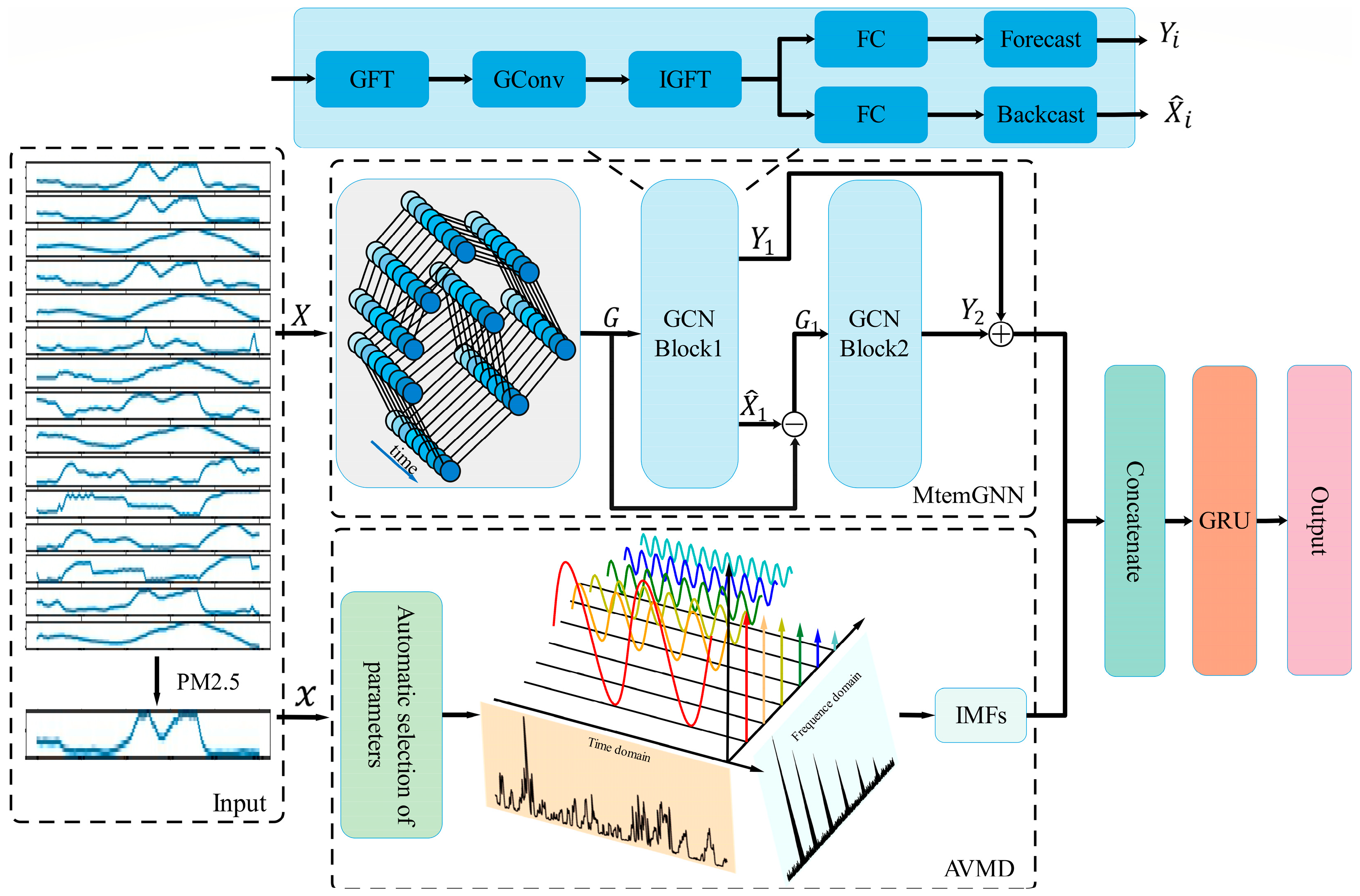
Figure 1. The structure of the PMNet.
Sustainability 14 13191 g001
Figure 2. The decomposition steps of AVMD.
Sustainability 14 13191 g002
Figure 3. The visualization of different degrees of mode mixing and abrupt change in the minimum value of K. (a) IMF with almost no mode mixing; (b) IMF with serious mode mixing; (c) Low-frequency large-value IMFs affecting other frequency band division when the value of K is too small; (d) AMME anomaly caused by excessively small value of K.
Sustainability 14 13191 g003
Figure 4. The establishment of graph structure.
Sustainability 14 13191 g004
Figure 5. Visualization of original signals and IMFs.
Sustainability 14 13191 g005
Figure 6. Visualization of mode mixing of two typical IMFs. (a) Low mode mixing degree of large amplitude IMFs; (b) Small amplitude IMFs tolerating a certain degree of mode mixing.
Sustainability 14 13191 g006
Figure 7. Comparison of partial real value tracking curves of different models.
Sustainability 14 13191 g007
Figure 8. Scatter plot comparison of different models.
Sustainability 14 13191 g008
Figure 9. Comparison of partial real value tracking curves of ablation experiment.
Sustainability 14 13191 g009
Figure 10. Scatter plot comparison of ablation experiment.
Sustainability 14 13191 g010
Table 1. The main parameters of PMNet.
Parameter NameValue
Initial learning rate0.001
Epochs150
Batch size24
Loss functionMean squared error (MSEloss)
OptimizerRoot Mean Square Propagation (RMSProp)
Window size24 h
Forecast horizon12 h
Table 2. The results of different models for PM2.5 concentration prediction in different time periods.
MethodsMetric+1 h+2 h+3 hAverage
StemGNNMAPE(%)16.12622.16730.21222.835
MAE2.0143.2684.7263.336
RMSE2.9175.2287.8085.681
LSTMMAPE(%)11.99119.33224.61818.647
MAE1.7282.7553.9112.798
RMSE2.5984.8117.0015.129
GRUMAPE(%)12.59417.51325.68818.598
MAE1.8022.8054.0592.889
RMSE2.7904.6976.9905.122
PMNetMAPE(%)5.4015.1125.1035.205
MAE0.5580.6460.6660.623
RMSE0.7310.8550.8630.816
Table 3. A comparison of the average effect of different models predicting PM2.5 in the next 12 h.
MethodsMAPE (%)MAERMSE
PMNet7.3480.8341.201
w/o MtemGNN11.9091.4031.978
w/o GRU26.0203.1684.387
w/o AVMD61.7118.45914.454
Table 4. The recent studies on PM2.5 forecasting.
Authors and Ref.Forecast HorizonData SourcesOutcomeAlgorithms
Huang et al. [30]One hourBeijingRMSE = 11.372EMD-GRU
Li et al. [31]One dayBeijingRMSE = 1.2289CEEMDAN-DSE-BVMD-CSA-KELM 1
Yang et al. [48]One hourXi’anRMSE = 0.8909AIVMD-RBF-IOWA-LSTM-EC 2
Gao et al. [49]One hourGansu RMSE = 3.405Graph-based Long Short-Term Memory (GLSTM)
Zhu et al. [50]One hourShanghaiRMSE = 4.24891D-CNN-biLSTM
Lei et al. [51]One hourMacaoRMSE = 3.72Random forest (RF)
Ho et al. [52]One dayKoreaRMSE = 8.2LSTM
Yeo et al. [53]One hourSeoulRMSE = 7.962CNN-GRU
1 Complete ensemble empirical mode decomposition with adaptive noise (CEEMDAN), differential symbolic entropy (DSE), variational mode decomposition improved by butterfly optimization algorithm (BVMD), and kernel extreme learning machine optimized by crow search algorithm (CSA-KELM). 2 Agreement index variational mode decomposition (AIVMD), radial basis function neural network (RBF), induced ordered weighted averaging (IOWA) operator, long short-term memory neural network (LSTM) and error correction (EC).
Publisher’s Note: MDPI stays neutral with regard to jurisdictional claims in published maps and institutional affiliations.