The SEIR Dynamic Evolutionary Model with Markov Chains in Hyper Networks

Abstract

In real life, individuals play an important role in the social networking system. When an epidemic breaks out the individual’s recovery rate depends heavily on the social network in which he or she lives. For this reason, in this paper a nonlinear coupling dynamic model on the hyper network was built. The upper layer is the dynamic social network under the hypernetwork vision, and the lower layer is the physical contact layer. Thus, the dynamic evolutionary coupling mechanism between the social network and epidemic transmission was established. At the same time, this paper deduced the evolution process of the dynamic system according to the Markov chain method. The probability equation of the dynamic evolution process was determined, and the threshold of epidemic spread on the non-uniform network was obtained. In addition, numerical simulations verified the correctness of the theory and the validity of the model. The results show that an individual’s recovery state will be affected by the individual’s social ability and the degree of information forgetting. Finally, suitable countermeasures are suggested to suppress the pandemic from spreading in response to the coupling model’s affecting factors.

1. Introduction

The intricate interactions between human behavior and its determinants (such as information acquisition, risk perception, perceived advantages, and costs of diverse behaviors) and the spread and control of infectious diseases are persistent study topics in epidemic diseases. People have achieved significant advancements in the study of epidemiology along with the evolution of society. In 1927, W.O. Kermack et al. [1] first proposed the classic warehouse model, which included three states: susceptible state, infection state, and recovery state. This model has been applied broadly so far. Later, under the inspiration of this model, more and more scholars carried out further research on this model and built the SEIR model with a latent state, and a SIS model that can be infected again, etc. [2,3,4]. A major factor in the spread of epidemics is human behavior. To improve control effects, it may be necessary to better understand how behavior affects the spread of disease, particularly when it comes to the human-to-human information sharing that occurs in the dual-network mode that includes the transmission layers of awareness and epidemics [5,6,7,8,9,10]. Among them, the research in [5] has shown that in places with large populations, individual awareness has a certain inhibitory effect on the scale of epidemic outbreaks, and even completely prevents the spread of the epidemic. In places with sparse populations, there is less exposure to the epidemic. The outbreak’s minimal effects demonstrate the importance of word-of-mouth propagation for the epidemic’s spread to some extent. According to the research in [8], the risk information that people have access to significantly affects how infectious diseases spread and develop.

Initially, people explored the process of epidemics in the context of complex networks [11,12,13] and explored how neighboring nodes affected the structure of the network by using a common infectious disease dynamics model. However, with the development of science and technology and the emergence of the high-speed rail network communication between people has further deepened. However, at the same time, these factors cause pandemics to spread more quickly once they start. Therefore, scholars’ research on the spread of epidemics is not limited to single-layer networks but has turned to research on the spread of epidemics in multiple networks [14,15,16,17]. In order to investigate the impact of individual awareness on the transmission of infectious diseases through Markov chains, a two-layer infectious disease model was developed in [15]. This study showed that individual awareness is related to the threshold of epidemic transmission. Multilayer networks, which are commonly unidirectional or bidirectional models between human social activities and disease transmission, study the interaction between the two layers to further explore the significance of disease to individuals in society. In multiple networks, scholars use the Markov chain method [18,19,20,21,22] and the average approximate field theory to dynamically analyze the model. They can study the outbreak process and the communication situation by collecting the percentages of the various states throughout each period. Then, particular countermeasures are suggested for the effect of awareness on the scope of communication. For example, when the new crown pneumonia broke out in 2019, the government reported the spread of the epidemic and adopted corresponding measures, such as home isolation, to quickly control the spread of the epidemic and ensure people’s life and health to the greatest extent. With the rapid development of information today, the role of social networks in the spread of epidemics cannot be ignored. Social media is the channel for most people to obtain information.

The accuracy and timeliness of the media’s coverage of epidemics are vital to the spread of epidemics [23,24,25,26,27], and it is a positive way for people. The study in [23] demonstrated the involvement of the media in the spread of an epidemic: social media can be very helpful in preventing the spread of an epidemic by increasing people’s sensitivity to environmental changes and, in turn, boosting awareness of the risk of infection to some level. Meanwhile, the measure is still a negative measure that can cause a certain amount of interference: we need to avoid being deceived by false information. In the social network system, the appearance of individual knowledge and information will have an antagonistic effect, and the ability to correctly identify information can play a positive role in preventing the spread of the epidemic [28,29]. Due to the existence of individual heterogeneity, various factors in social networks will not only affect the outbreak of epidemics. Similarly, the spread of epidemics will also have a corresponding impact on the social behavior of individuals [30,31,32]. In [30], the authors considered the impact of asymptomatic infected individuals and individual heterogeneity on the spread of the epidemic, and then further enriched the study by discussing and comparing two cases, making the article more relevant. Therefore, researchers have proposed a dual-layered infectious disease coupling mechanism. According to the study in [33], the researchers found through the construction of a multi-network coupling model and associated simulation experiments that people’s awareness will vary depending on their personal states, and weak information awareness will cause a pandemic outbreak. Unlike complex social networks, this paper describes the dynamic social network process under the vision of the hyper network to portray the interrelationship between multiple nodes and to construct a two-layer coupling mechanism. The spreading threshold of the epidemic is determined using the Markov method and dynamics as a theoretical foundation. Finally, simulation experiments support the theory’s veracity and the model’s efficacy further.

The contributions of this article are as follows:

(1)

With the support of the microscopic Markov theory, a two-layer SEIR (Susceptible-Exposed-Infected-Recovered) model including the coupling of the information layer and the physical contact layer is proposed. An interacting relationship exists between the model’s layers;

(2)

A social network model is constructed under the hyper network vision, including three dynamic evolution processes: the addition of hyperedges, the disappearance of hyperedges, the entry, and the exit of nodes;

(3)

Taking into account the heterogeneity and time-varying of individuals, the probability of node state transition in this study is no longer a fixed constant, but a time-varying parameter affected by the current state and degree of each node;

(4)

The effects of different parameters are tested in turn. The simulation results show that the strength of social networks has a certain impact on the recovery of individuals. As a result, the person’s social abilities can be adequately enhanced.

The rest of this article is organized as follows: the second part is the theoretical background of the model, the third part is the construction of the model of the coupling mechanism, the fourth part is the simulation analysis using MATLAB, and the fifth part is the conclusion and prospects.

2. Theoretical Background

This part includes an introduction to some of the paper’s parameters, a description of the theoretical context, and a presentation of the model that was established for this paper. An introduction to the relevant parameters and their physical meanings in the paper is given in

Table 1. Parameters and their physical meanings in simulation experiments.

Parameter	Physical Meanings
$\theta$	Probability of transition from state S to state E
$\beta$	Probability of transition from state E to state I
$\gamma$	Probability of transition from state I to state R
$\eta$	Probability of transition from conscious social to unconscious social
$\delta$	Probability of forgetting information
$\lambda$	Probability of not spreading information
$w^A$	Probability of individual awareness activity intensity
$s^{*}$	Social intimacy threshold

.

2.1. Hyper-Graph and Hyper-Network

Let $V=\{v_1,v_2,\dots ,v_n\}$ be a finite set, $E_i=\{v_{i1},v_{i2},\dots ,v_{ij}\},(v_{ik}\in v,k\in N^{*})$ is a family of non-empty subsets of $V$, and $E^h=\{E_1,E_2,\dots ,{\mathrm{E}}_m\}$ represents the set of hyperedges, then we define the binary relation $H=\{V,E^h\}$ as a hypergraph. The characteristic of a hypergraph is that it can contain any number of nodes, so it is more suitable for real life. Hypernetworks are complex systems described by hypergraphs. In other words, a hypernetwork is a network system made up of a collection of hyper-edges and hyper-nodes. The non-uniform hypergraph is used in this article.

2.2. Social Networks

Social networking plays an important role in people’s lives. It has become a part of people’s lives and has an inestimable impact on people’s information acquisition, thinking, and life. At the same time, it has become a window for people to obtain information, show themselves, and promote marketing. In the social network system, everyone is both the recipient and creator of information and is subject to change and uncertainty. Therefore, this paper proposes a dynamic social network with three deductive modes under the hyper network [34]. 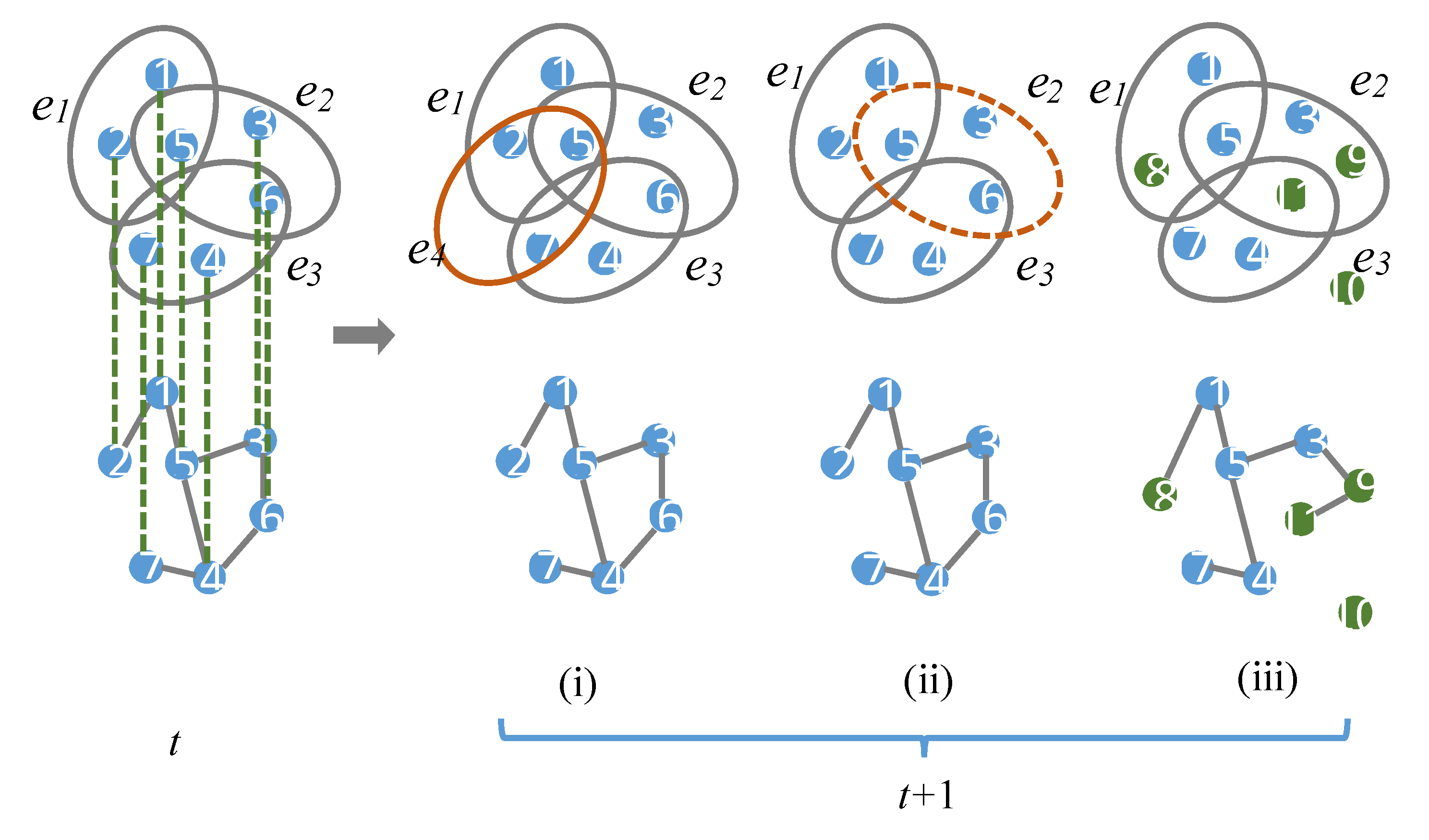As shown in Figure 1, the model includes the following three dynamic processes: (1) the addition of hyper edges; (2) the disappearance of hyperedges; and (3) the entry and exit of nodes.

In real life, these three dynamic evolutionary processes often happen to everyone. For example, when a person joins a new group, a new social network relationship—or new hyperedge—is formed with the members of the new group. The disappearance of the hyperedge can be described as when the relationship between the individual and the existing individual within the hyperedge is broken so that a good social environment cannot exist between the two, and the hyperedge of the social network disappears. The node’s entry and exit mean that there is still a constant flow of new people joining social network systems where there is a relationship between the old person and the current network. For example, when an individual is in a company, it often happens that the old individual resigns, and the new individual enters. In this way, the existing social network of colleague relations will be changed accordingly.

The upper layer of the model is the social network layer, and the lower layer is the individual activity layer. There is a one-to-one correspondence between the two layers of networks. At time t, there are seven individuals (1–7) in the upper system of the model and three hyperedges ($e_1~e_3$) containing these individuals; the individuals in the lower network system are connected by links. At time t + 1, the system will perform the following situations with a certain probability: (i) add $m=1$ hyperedge with probability $p$, and the hyper-edge $e_4$ is represented by an orange solid line; (ii) delete $m=1$ hyper-edge with probability $q$, the deleted hyper edge $e_2$ is represented by orange dashed line; (iii) add $u=4$ (8–11) new nodes with probability $1-p-q$ and delete $m_1=2$ (2, 6) original individuals and their links, at the same time some new nodes are added to the existing hyperedges in the system, and the newly entered nodes are shown in green.

In the social network system, the degree of node and the degree of hyper edge, respectively, describe the number of nodes connected by the hyper edge and the number of hyperedges containing the node and characterize the strength of the individual’s aware activity and the individual’s social ability. The more hyperedges an individual is connected to, the stronger the individual’s social connections, which means that he or she will have stronger social skills in the social network. Here, the following equation is used to describe the individual’s active intensity and social skills:

$$w(d_j(t,t_i))=\frac{d_j(t,t_i)}{\max (d(t))}$$

(1)

where $d_j(t,t_i)$ represents the node degree.

$$w(h_j(t,t_i))=\frac{h_j(t,t_i)}{\max (h(t))}$$

(2)

Among them, $h_j(t,t_i)$ represents the node over-degree. For the sake of simple calculation, $w(h_j(t,t_i))$ is abbreviated as $w^A$ here.

Individual social networks are not formed for nothing, whether it is introductions to friends, passive social interaction, etc. Therefore, the social ability of an individual is divided into aware socializing $w^A$ and unaware socializing $w^U$ where $w^U=\mu w^A$, $\mu \in (0,1)$ is the conversion coefficient.

2.2.1. Jaccard Similarity Coefficient

It is common knowledge that a person’s personality, temperament, and other characteristics are all influenced by their social network environment. In addition, his social network is made up of individuals with the same personality. For example, more self-disciplined people are more likely to be friends with people who have a planned life, and people who have irregular lives are more difficult to have the same social network environment. People are always more likely to be in the same social network environment with people who are similar to them. In a social network, if individuals $i$ and $j$ have more common neighbor nodes, it means that individuals $i$ and $j$ have a closer social circle, and the higher the similarity between users, is the easier it is to become close friends, and then enrich your social network system. Given this, this paper uses the Jaccard similarity coefficient [35] to calculate the connection strength based on the number of common neighbors.

$$s_j=\frac{\max \_s_j}{sum(s_j)}$$

(3)

Equation (3) is described as traversing all the social network systems of node $j$, further calculating the public nodes of node $j$ and other nodes, selecting the largest number of public nodes($\max \_s_j$), and calculating the number of nodes in common between node $j$ and other nodes (except node $j$).

2.2.2. Node Connection Probability

Individual heterogeneity is the differences between individuals, including personality, temperament, and so on. In the complex social network, the heterogeneity of individuals makes social network relationships no longer describable by a fixed parameter. Therefore, it is not only their factors that will affect the social relationship between individuals and other new individuals, but also the characteristics of other new individuals. It is crucial for the development of social networks. Therefore, the probability of forming a social network relationship between individual $j$ and other individuals consists of two parts, one is the individual’s social ability, and the other is the degree of intimacy between individuals, that is:

$$w=\left\{\begin{array}{cc}{s}^{*}& s_j<s^{*}\\ \frac{h_j(t,t_i)+1}{{\displaystyle \sum _j{h}_j(t,t_i)+1}}+s_{\mathrm{j}}& s_j\ge s^{*}\end{array}\right.$$

(4)

where $s^{*}$ is the boundary value. We establish a lower bound on the closeness between individuals to prevent a scenario in which the closeness is zero.

2.3. SEIR Model

2.3.1. DB Policy Updates Mechanism

When a user posts new information on a social network, the network’s ability to spread that information depends heavily on how other users respond, whether they forward the information or not. For an individual, whether to forward information is affected by many factors, including the user’s interest in the content of the information, and his/her neighbors’ users’ interest in information forwarding. In other words, the likelihood that the person will transfer the information will be considerably increased if they believe that their neighbors will do so.

DB (Death–Birth) strategy update mechanism: randomly select a node, first abandon its strategy, and then select its neighbor strategy with a probability proportional to the fitness. For the sake of simplicity, the neighbors here will be defaulted to not carry out information dissemination. For each individual, a piece of information contains two cases of spreading and non-spreading, that is, spreading $S_f$ and non-spreading as $S_n$. Let the initial social network have $k_f$ propagation nodes, then the initial income matrix is:

$$U=\left[\begin{array}{cc}{u}_{ff}& u_{fn}\\ u_{nf}& u_{nn}\end{array}\right]$$

(5)

Here, the information content is an epidemic-related topic, and the information content is closely related to people. Then forwarding the information can effectively prevent the spread of the epidemic. The corresponding income matrix has the following characteristics: $u_{ff}>u_{fn}>u_{nn}$. Therefore, let $u_{ff}=0.5,u_{fn}=u_n{}_f=0.3,u_{nn}=0.2$.

The fitness function represents the size of an individual’s interest in disseminating information. The fitness function used in this article is as follows: $\pi =1-\alpha +\alpha ·A$.

Among them, $A$ represents the individual’s income, which is determined by the information forwarding between the individual and its neighbors. According to the evolutionary dynamics, the fitness of the central user who adopts the strategies $S_f$ and $S_n$ can be expressed as:

$${\pi }_f=1-\alpha +\alpha [k_f·u_{ff}+(N-k_f)·u_{fn}]$$

(6)

$${\pi }_n=1-\alpha +\alpha [k_f·u_{fn}+(N-k_f)·u_{nn}]$$

(7)

where $N$ is the total number of individuals in the network. According to the DB policy update mechanism, according to the above information, the probability of not disseminating information is

$$P_n=\frac{(N-k_f)·{\pi }_n}{k_f·{\pi }_f+(N-k_f)·{\pi }_n}=\lambda .$$

(8)

2.3.2. SEIR Model

Epidemics can be spread via the air, water, food, contact, soil, vertical transmission, etc. To stop some illnesses from spreading, the epidemic prevention department must stay up to date on their incidence and take prompt action. In the pre-epidemiological time, the combined transmission of disease and information was taken into consideration, but it tended to concentrate on single-layer networks [36,37]. Different networking layers were involved in both the spread of disease and the propagation of information. Granell et al. [38] therefore attempted to research the coupled dynamics behavior on two-layer networks with the dissemination of disease information and the propagation of disease. The SEIR (Susceptible-Exposed-Infected-Recovered) model with individuals with latent states is constructed here [39,40]. As shown in Figure 2:

Among them, the letter $S$ stands for susceptible individuals, which are those who have not gotten the disease, but lack immunity and are susceptible to infection after contact with infected persons; the letter $E$ stands for latent individuals, which refers to persons who have been exposed to infections and have a certain probability of transforming into the category $I$ individuals; the letter $I$ represents infected individuals, which refers to a person infected with an infectious disease, which can be transmitted to a member of the $S$ category, turning it into an $E$ or $I$ individual; the letter $R$ represents a recovered individual, and refers to a person who has recovered from the disease and has immunity. For each individual, the cognition of its state is not completely clear. Therefore, it is divided into aware individual (Awareness) and unaware individual (Unawareness) according to the individual’s awareness.

According to the above diagram, the individual state transition can be described as the susceptible individual $S$ becoming a latent individual with probability $\theta w^A$, the latent individual $E$ becoming an infected individual with probability $\beta$, and the infected individual $I$ transforming into a recovered individual $R$ with probability $\gamma$. The aware individual $A$ can be transformed into unaware individual $U$ with probability $\delta \lambda$, where $\delta$ is the probability that the individual forgets the disease information and $\lambda$ is the probability of not disseminating information in the DB strategy update mechanism, that is, the awareness of information dissemination is weak. At the same time, the unaware individual $U$ can also be transformed into aware individual $A$ with probability $1-r_i(t)$ and $r_i(t)$ is the infection attenuation factor, that is, the probability of knowing the infection probability, and the node status is not changed when the node status is $U$. When $x>0$, the value of $H(x)$ is 1, otherwise, the value of $H(x)$ is 0, that is, unknowing individuals will be aware of the epidemic through their neighbors. It can be seen from the above model that the upper and lower state couplings can have the following eight state individuals: aware susceptible individuals AS (Aware Susceptible), aware exposed individuals AE (Aware Exposed), aware infected individuals AI (Aware Infectious), and aware recovered individuals AR (Aware Recovered), unaware susceptible individuals US (Unaware Susceptible), unaware exposed individuals UE (Unaware Exposed), unaware infected individuals UI (Unaware Infectious), and unaware recovered individuals UR (Unaware Recovered).

3. Discussion

According to the dynamic evolution mechanism of social networks and the spread of epidemics, this paper constructed a two-way coupling mechanism as shown in Figure 3. In the coupling model, the upper layer represents the individual behavior layer, and the lower layer is the physical contact layer. The degree of information forgetting, and the person’s social aptitude are used to achieve the two-way influence. This article assumes that the total number of nodes in the hyper network is $N(t)$, and each hyper edge contains $\mu +1$ nodes.

The hyper-degree $h_j(t,t_i)$ is a continuous real variable that may be affected by the process (1)–(3). Therefore, $h_j(t,t_i)$ satisfies the following kinetic equation:

(i)

Addition of hyper edges

$$\frac{\partial h_j(t,t_i)}{\partial t}=pm·({\lambda }_1-{\lambda }_2)·\frac{1}{N(t)}+pm·({\lambda }_1-{\lambda }_2)·u·w$$

(9)

The first item on the right represents a random selection of a node among $N$ nodes while selecting $u$ nodes in the original network system to link $m$ new hyperedges with probability $p$. Where ${\lambda }_1$ describes the entry rate of the node, ${\lambda }_2$ describes the exit rate of the node, and w represents the link probability between nodes. Duplicate hyper edges are not allowed.

(ii)

Deletion of hyper-edge

$$\frac{\partial h_j(t,t_i)}{\partial t}=qs·({\lambda }_1-{\lambda }_2)·(-\frac{1}{N(t)})+qs·({\lambda }_1-{\lambda }_2)·u·(-w)$$

(10)

The first item on the right represents the random selection of a node from $N$ nodes and deleting it, and at the same time selecting $u$ nodes on the same hyper edge as the node to delete $s$ ($s<m$) new hyper edges with probability $q$. Duplicate hyper edges are not allowed.

(iii)

Entry and exit of nodes

$$\frac{\partial h_j(t,t_i)}{\partial t}=(1-p-q)\left\{{\lambda }_2·(-\frac{m_1}{N(t)})+{\lambda }_1·u·w\right\}$$

(11)

The process evolves with a probability of $1-p-q$. The first item on the right indicates that $m_1$ nodes are randomly selected from $N$ nodes for deletion, and $u$ new nodes are flooded into the social network system to join the original hyper edge.

In summary, we can obtain:

$$\begin{array}{l}\frac{\partial h_j(t,t_i)}{\partial t}=({\lambda }_1-{\lambda }_2)·(pm-qs)·\frac{1}{N(t)}+(1-p-q)·{\lambda }_2·(-\frac{m_1}{N(t)})\\ \hspace{1em}\hspace{1em}\hspace{1em}+\left\{pm·({\lambda }_1-{\lambda }_2)-qs·({\lambda }_1-{\lambda }_2)+(1-p-q){\lambda }_2\right\}·u·w\end{array}$$

(12)

where $N(t)=({\lambda }_1-{\lambda }_2)·t$, ${\displaystyle \sum _j{h}_j(t,t_i)}\approx \left[pm-qs+(1-p-q)m_1\right]\times E\left[N(t)\right]$.

The above equation can be written as:

$$\frac{\partial h_j(t,t_i)}{\partial t}=\left\{A+\frac{B}{C}·(h_j(t,t_i)+1)\right\}·\frac{1}{t}+B·s_j$$

(13)

where $A=(pm-qs)-\frac{(1-p-q)·m_1·{\lambda }_2}{({\lambda }_1-{\lambda }_2)}$, $B=\left\{({\lambda }_1-{\lambda }_2)(pm-qs)+(1-p-q)·{\lambda }_1\right\}·u$, $C=\left[pm-qs+(1-p-q)m_1\right]\times ({\lambda }_1-{\lambda }_2)$.

By integrating at both ends, you can obtain:

$$h_j(t,t_i)=\left\{\frac{AC}{B}+(1-p-q)\right\}·{(\frac{t}{t_i})}^{\frac{B}{C}}-D+B·s_j·(t-t_i)$$

(14)

where $D=(1-p-q)-\frac{AC+B}{B}$, $h_j(t_i,t_i)=1-p-q$.

At time t, for the state of the jth node in the ith batch, there are one of the following eight states: $p_j^{AS}(t,t_i), p_j^{AE}(t,t_i), p_j^{AI}(t,t_i), p_j^{AR}(t,t_i)$, $p_j^{US}(t,t_i), p_j^{UE}(t,t_i), p_j^{UI}(t,t_i), p_j^{UR}(t,t_i)$ and $p_j^{AS}(t,t_i)+p_j^{AE}(t,t_i)+p_j^{AI}(t,t_i)+p_j^{AR}(t,t_i)+p_j^{US}(t,t_i)+p_j^{UE}(t,t_i)+p_j^{UI}(t,t_i)+p_j^{UR}(t,t_i)=1$. Assuming that the conversion probability of each node is independent of each other, we can obtain:

$$r_i(t)=H\{\xi -{\displaystyle {\sum }_j{a}_{ji}·P_j^A(t)}·w(d_j(t,t_i))\}$$

(15)

$$q_i^U(t)={\displaystyle \prod _j\left\{1-b_{ji}[P_i^I(t)+P_i^E(t)]·{\theta }^U\right\}}$$

(16)

$$q_i^A(t)={\displaystyle \prod _j\left\{1-b_{ji}[P_i^I(t)+P_i^E(t)]·{\theta }^A\right\}}$$

(17)

Among them, ${\theta }^A=\eta ·{\theta }^U$ is the local awareness threshold. $a_{ij}$ and $b_{ij}$, respectively, represent the adjacency matrix of the behavior diffusion layer and the physical contact layer at time t. When the probability of AI transitioning to AR is $r$, $q_i^A(t)$ represents the probability that the state of the aware node has not changed at time t, and similarly, $q_i^U(t)$ represents the probability that the state of the unaware node has not changed at time t.

According to the above content and Figure 2, this paper obtains the state transition probability tree. As shown in Figure 4, It describes the possible states and transitions of nodes in the hyper network. Each tree can be divided into three stages: the U-A process of the information diffusion layer and the S-E-I-R process of the physical contact layer. The eight roots of the tree represent the possible state of the node at time t and the node state transitions under a certain probability. The leaf represents the state that can be changed at t+1. In addition, the state transition matrix is also available, where both the row and column states of the matrix are: $\left[\begin{array}{cccccccc}US& UE& UI& UR& AS& AE& AI& AR\end{array}\right]$.

$$\left[\begin{array}{cccccccc}{r}_i\left(t\right)·w^U·q_i^U\left(t\right)& r_i\left(t\right)·w^U·(1-q_i^U\left(t\right))& 0& 0& (1-r_i\left(t\right))·w^A·q_i^U\left(t\right)& (1-r_i\left(t\right))·w^A·(1-q_i^U\left(t\right))& 0& 0\\ 0& r_i\left(t\right)·(1-\beta )& r_i\left(t\right)·\beta & 0& 0& (1-r_i\left(t\right))·(1-\beta )& (1-r_i\left(t\right))·\beta & 0\\ 0& 0& r_i\left(t\right)·(1-\gamma )& r_i\left(t\right)·\gamma & 0& 0& (1-r_i\left(t\right))·(1-\gamma )& (1-r_i\left(t\right))·\gamma \\ 0& 0& 0& 0& r_i\left(t\right)& 0& 0& 1-r_i\left(t\right)\\ \delta \lambda ·w^A{q}_i^U\left(t\right)& \delta \lambda ·w^A(1-q_i^U\left(t\right))& 0& 0& (1-\delta \lambda )·w^U{q}_i^A\left(t\right)& (1-\delta \lambda )·w^U(1-q_i^A\left(t\right))& 0& 0\\ 0& \delta \lambda ·(1-\beta )& \delta \lambda ·\beta & 0& 0& (1-\delta \lambda )·(1-\beta )& (1-\delta \lambda )·\beta & 0\\ 0& 0& \delta \lambda ·(1-\gamma )& \delta \lambda ·\gamma & 0& 0& (1-\delta \lambda )·(1-\gamma )& (1-\delta \lambda )·\gamma \\ 0& 0& 0& \delta \lambda & 0& 0& 0& 1-\delta \lambda \end{array}\right]$$

(18)

According to the state probability of each node at time t, the state transition probability tree and the Markov chain method can know the state probability of each node at t+1:

$$P_i^{US}(t+1)=P_i^{US}(t)·\left\{r_i(t)·w^U·q_i^U(t)\right\}+P_i^{AS}(t)·\left\{\delta \lambda ·w^U·q_i^U(t)\right\}$$

(19)

$$P_i^{AS}(t+1)=P_i^{US}(t)·\left\{\left[1-k_i(t)\right]·w^A·q_i^U(t)\right\}+P_i^{AS}(t)·\left\{(1-\delta \lambda )·w^A·q_i^A(t)\right\}$$

(20)

$$\begin{array}{l}{P}_i^{UE}(t+1)=P_i^{US}(t)·\left\{r_i(t)·w^U·(1-q_i^U(t))\right\}+P_i^{AS}(t)·\left\{\delta \lambda ·w^U·(1-q_i^U(t))\right\}\\ \hspace{1em}\hspace{1em}\hspace{1em}\hspace{1em}\hspace{1em}+P_i^{UE}(t)·\left\{r_i(t)·(1-\beta )\right\}+P_i^{AE}(t)·\left\{\delta \lambda ·(1-\beta )\right\}\end{array}$$

(21)

$$\begin{array}{l}{P}_i^{AE}(t+1)=P_i^{US}(t)·\left\{\left[1-r_i(t)\right]·w^A·(1-q_i^A(t))\right\}+P_i^{AS}(t)·\left\{(1-\delta \lambda )·w^A·(1-q_i^A(t))\right\}\\ \hspace{1em}\hspace{1em}\hspace{1em}\hspace{1em}\hspace{1em}+P_i^{UE}(t)·\left\{\left[1-r_i(t)\right]·(1-\beta )\right\}+P_i^{AE}(t)·\left\{(1-\delta \lambda )·(1-\beta )\right\}\end{array}$$

(22)

$$P_i^{UI}(t+1)=P_i^{UE}(t)·\left\{r_i(t)·\beta \right\}+P_i^{AE}(t)·\left\{\delta \lambda ·\beta \right\}+P_i^{UI}(t)·\left\{r_i(t)·(1-\gamma )\right\}+P_i^{AI}(t)·\left\{\delta \lambda ·(1-\gamma )\right\}$$

(23)

$$\begin{array}{l}{P}_i^{AI}(t+1)=P_i^{UE}(t)·\left\{\left[1-r_i(t)\right]·\beta \right\}+P_i^{AE}(t)·\left\{(1-\delta \lambda )·\beta \right\}\\ \hspace{1em}\hspace{1em}\hspace{1em}\hspace{1em}\hspace{1em}+P_i^{UI}(t)·\left\{\left[1-r_i(t)\right]·(1-\gamma )\right\}+P_i^{AI}(t)·\left\{(1-\delta \lambda )·(1-\gamma )\right\}\end{array}$$

(24)

$$P_i^{UR}(t+1)=P_i^{UI}(t)·\left\{r_i(t)·\gamma \right\}+P_i^{AI}(t)·\left\{\delta \lambda ·\gamma \right\}+P_i^{UR}(t)·\left\{r_i(t)\right\}+P_i^{AR}(t)·\left\{\delta \lambda \right\}$$

(25)

$$P_i^{AR}(t+1)=P_i^{UI}(t)·\left\{\left[1-r_i(t)\right]·\gamma \right\}+P_i^{AI}(t)·\left\{\left[1-\delta \lambda \right]·\gamma \right\}+P_i^{UR}(t)·\left\{1-r_i(t)\right\}+P_i^{AR}(t)·\left\{1-\delta \lambda \right\}$$

(26)

When $t\to \infty$, the infection rate is close to the threshold, the number of infected individuals is very small, and the system enters a stable state, for example, for all nodes, there is $p_i(t+1)=p_i(t)$. Individuals first transition from the infected state to the $E$ state after being infected, and the threshold of disease is given by $p^E$. As the system reaches stability, the probability of the node being infected tends to 0, assuming $P_i^E={\epsilon }_i<<1$, ignoring higher-order terms, according to Equations (12)–(17), the state transition probability is described.

$$\begin{array}{l}{q}_i^U(t)={\displaystyle \prod _j\left\{1-b_{ji}\left[P_i^I(t)+P_i^E(t)\right]·{\theta }^U\right\}}\approx 1-{\displaystyle \sum _j{b}_{ji}}(P_i^I(t)+P_i^E(t))·{\theta }^U\\ \hspace{1em}\hspace{1em}=1-{\displaystyle \sum _j{b}_{ji}}(\frac{\beta }{\gamma }{P}_i^E(t)+P_i^E(t))·{\theta }^U\\ \hspace{1em}\hspace{1em}=1-{\tau }_i^{\prime }(1+\frac{\beta }{\gamma })\end{array}$$

(27)

$$\begin{array}{l}{q}_i^A(t)={\displaystyle \prod _j\left\{1-b_{ji}\left[P_i^I(t)+P_i^E(t)\right]·{\theta }^A\right\}}\approx 1-{\displaystyle \sum _j{b}_{ji}}(P_i^I(t)+P_i^E(t))·{\theta }^A\\ \hspace{1em}\hspace{1em}=1-{\displaystyle \sum _j{b}_{ji}}(\frac{\beta }{\gamma }{P}_i^E(t)+P_i^E(t))·\eta {\theta }^U\\ \hspace{1em}\hspace{1em}=1-{\tau }_i·\eta \end{array}$$

(28)

where ${\tau }^{\prime }={\displaystyle \sum _j{b}_{ji}}·P_i^E(t)·{\theta }^U$, $\tau ={\displaystyle \sum _j{b}_{ji}}·P_i^E(t)·{\theta }^U·(1+\frac{\beta }{\gamma })$.

In the steady state, $q_i^A(t)$ and $q_i^U(t)$ can be described as $q_i^A(t)=1-\eta \tau$ and $q_i^U(t)=1-\tau$, therefore:

$$\begin{array}{l}{P}_i^E(t+1)=P_i^{AE}(t+1)+P_i^{UE}(t+1)\\ \hspace{1em}\hspace{1em}\hspace{1em}\hspace{1em}=P_i^{AS}(t)·\left\{(1-\delta \lambda )·w^A·(1-q_i^A(t))+\delta \lambda ·w^A·(1-q_i^U(t))\right\}\\ \hspace{1em}\hspace{1em}\hspace{1em}\hspace{1em}+P_i^{US}(t)·\left\{r_i(t)·w^U·(1-q_i^U(t))+\left[1-r_i(t)\right]·w^U·(1-q_i^A(t))\right\}\\ \hspace{1em}\hspace{1em}\hspace{1em}\hspace{1em}+P_i^E(t)·(1-\beta )\end{array}$$

(29)

The above equation can be simplified as:

$$\begin{array}{l}{\epsilon }_i=P_i^{AS}(t)·\left\{(1-(1-\eta \tau ))·w^A·(1-\delta \lambda )+\delta \lambda ·w^U·(1-(1-\tau ))\right\}\\ \hspace{1em}+P_i^{US}(t)·\left\{r_i(t)·w^U·(1-(1-\tau ))+\left[1-r_i(t)\right]·w^A·(1-(1-\eta \tau ))\right\}\\ \hspace{1em}+{\epsilon }_i·(1-\beta )\end{array}$$

(30)

In summary, when the steady state is reached, $P_i^A\approx P_i^{AS}$ and $P_i^U\approx P_i^{US}$. Thus, the Equation (30) can be transformed into:

$${\epsilon }_i=P_i^A(t)·\left\{\eta \tau ·w^A·(1-\delta \lambda )+\delta \lambda ·w^U·\tau \right\}+P_i^U(t)·\left\{r_i(t)·w^U·\tau +\left[1-r_i(t)\right]·w^A·\eta \tau \right\}+{\epsilon }_i·(1-\beta )$$

(31)

Simplify to obtain:

$$\begin{array}{l}\beta {\epsilon }_i=P_i^A(t)·\eta \tau +P_i^U(t)·\tau \\ \hspace{1em} =P_i^A(t)·\eta \tau +(1-P_i^A(t))·\tau \\ \hspace{1em} =\left[1-(1-\eta )·P_i^A(t)\right]·{\displaystyle \sum _j{b}_{ji}}·{\theta }^U·(1+\frac{\beta }{\gamma })·{\epsilon }_i\end{array}$$

(32)

At the same time, the above formula can still be transformed into:

$${\displaystyle \sum _j\left\{\left[1-(1-\eta )·P_i^A(t)\right]·b_{ji}·(1+\frac{\beta }{\gamma })-\frac{\beta }{{\theta }^U}·t_{ij}\right\}·}{\epsilon }_j=0.$$

(33)

where $t_{ij}$ is an element in the identity matrix. Let $h_{ij}=\left[1-(1-\eta )·P_i^A(t)\right]·b_{ji}·(1+\frac{\beta }{\gamma })$ be the element of matrix $H$, and ${\mathsf{\Lambda }}_{\max }(H)$ be the maximum eigenvalue of matrix $H$. According to Equation (33), the epidemic threshold in this model is:

$${\beta }^c=\frac{\beta }{{\mathsf{\Lambda }}_{\max }(H)}.$$

(34)

4. Simulation

This section will further analyze the proposed dynamic evolution model through simulation. The proportion of recovered individuals in the steady state is the most critical indicator of the epidemic, and it can be defined as ${\rho }^R=\frac{N^R}{N}$, where $N^R$ and $N$ represent the number of recovered individuals and all individuals in the model, respectively. Similarly, in order to better measure the effectiveness of the inter-layer parameters, this article defines the proportion of aware individuals as ${\rho }^{RA}=\frac{N^{RA}}{N}$, where $N^{RA}$ and $N$ represent the number of aware infected individuals and the total number of network systems, respectively.

4.1. Influence of Parameters within the Layer

First, a simulation experiment was performed on the correlation between the relevant parameters in the lower physical contact layer in the model and the proportion of recovered individuals. The results are shown in Figure 5. When the proportion of recovered individuals was higher, the color tended to be brighter yellow. On the whole, the highest proportion of recovered individuals was set at 0.9. As the conversion rate $\beta$ increased, the increase in the proportion of recovered individuals can be seen with the naked eye. In Figure 5a, although the infection rate ${\theta }^A$ and recovery rate $\gamma$ both reached 1, the proportion of recovered individuals still did not reach 0.7. Looking at Figure 5c, when the infection rate ${\theta }^A$ and recovery rate $\gamma$ were only 0.4, the proportion of individuals reached 0.7852. This shows that in the same social environment, the greater the rate at which an individual’s exposed state turns to an infected state, the faster it will be to seek medical attention, which will result in a higher proportion of individuals recovering within a unit of time. Observing Figure 5b, when the individual infection rate ${\theta }^A$ was constant at 0.6, as the recovery rate $\gamma$ increased, it can be seen that the proportion of recovered individuals gradually changed from blue to bright yellow, which shows that when the individual faces the same infection rate, due to individual heterogeneity, individuals have different recovery abilities, and as the recovery rate of the individual increases, the more individuals recover per unit time. Similarly, when the recovery rate $\gamma$ was constant at 0.6, the same law mentioned above was in place.

4.2. The Influence of Parameters between Layers

4.2.1. Information Forgetting and Dissemination Options

The ability of individuals to disseminate information and the ability to forget information has a certain impact on whether other individuals are aware of epidemics and take corresponding measures. For this reason, this article conducted related simulation experiments to further verify the above statements. The results are shown in Figure 6. On the whole, when $\delta$ and $\lambda$ were both 0, all recovered individuals are aware recovered individuals, and there was no further transition to unaware recovered individuals. In Figure 6a, when both $\delta$ and $\lambda$ were 0, and the recovery rate was $\gamma =0.1$, the proportion of recovered individuals was 0.6324; In Figure 6b, when the recovery rate was $\gamma =0.2$, the proportion of recovered individuals was 0.7293; In Figure 6c, when the recovery rate was $\gamma =0.3$, the proportion of recovered individuals was 0.8172. It can be seen that under the same conditions, the higher the recovery rate, the greater the proportion of recovered individuals, which further verifies that the recovery rate is critical to the spread of epidemics. In this regard, targeted measures can be taken to increase the recovery rate of individuals, thereby effectively preventing the outbreak of the epidemic.

It can be seen in Figure 6 that the rate of individual information forgetting $\delta$ and the choice of information dissemination were inversely proportional to the proportion of aware restored individuals, and the closer the edge was the higher the proportion of aware individuals. That is, when the individual forgets information faster, the aware recovery individual is more likely to become an unaware recovery individual within a unit of time. It can be seen in the Figure 6a that when the individual’s ability to communicate with information remains unchanged, the more the information is forgotten, the more aware individuals turn into unaware individuals. Therefore, the proportion of aware individuals gradually decreases. Similarly, the choice of information has the same law. In addition, on Figure 6b, when $\lambda =0.005,\delta =0.6$, aware recovered individual ${\rho }^{RA}=0.6963$; when $\delta =0.005,\lambda =0.6$, aware recovered individual ${\rho }^{RA}=0.7003$, there was a slight difference between the two, which means that these two factors have different effects on the recovery of the individual. At the same time, it can be said that the individual’s choice of information is more important than the level of forgotten information.

4.2.2. Individual Social ability and Information Forgetting

In the two-way coupling model constructed in this article, the social ability of the individual in the upper layer penetrates into the physical contact layer, and the strength of the social ability has a certain impact on the individual’s state transition. Similarly, individual information forgetting has a corresponding effect on the construction of individual social networks. The role of the new hyperedge, or the entry of new individuals, etc. Looking at Figure 7 as a whole, when $\delta =0.1$, the proportion of aware individuals in the Figure 7a–c increased from 0.7602 to 0.7782 and then to 0.8022, which further confirmed the influence of the restoration of individuals on the proportion of aware individuals under the same conditions. In Figure 7b, when $w^A=0.6$, $\delta$ was 0.1, 0.25, and 0.5, the proportion of individuals in ${\rho }^{RA}$ was 0.7642, 0.7023, and 0.654, respectively. It can be seen that the proportion of individuals who aware recover was negatively correlated with the degree of information forgetting. This means that the greater the degree of individual information forgetting, the more aware recovery individuals will transition to unaware recovery individuals. On the contrary, when $\delta =0.25$, when individual social ability $w^A$ was selected as 0.1, 0.4, 0.8, the proportion of aware restored individuals was 0.1459, 0.6923, and 0.7203, respectively. This can be explained as the increase in the individual’s social abilities and the impact on the individual’s social range. The choice has changed, so the individual’s state has a corresponding change. It can be seen from the above model that enhancing the individual’s own social skills can effectively increase the proportion of recovered individuals.

In order to further verify the impact of social ability and information forgetting on the recovery of individuals, this article uses Figure 8 to further explain. Observing the color changes of Figure 8a–c, we can see that the individual’s social ability is positively correlated with the proportion of recovered individuals, while the degree of individual information forgetting is negatively correlated with aware recovered individuals.

5. Conclusions

This paper proposed an epidemic model under a hyper network vision. In this model, in order to describe the interaction between multiple individuals, the upper layer uses a hyper network structure to portray the evolution of social networks while the lower layer is used to describe the spread of epidemics. With the theoretical support of the hyper network system and Markov chain method, this paper derived the epidemic threshold, and through simulation analysis, the validity of the model was further confirmed. The results of the experiment suggested that social ties affect the spread of the disease. People can use a variety of strategies to relieve the pressure of disease transmission after being inspired by this conclusion. In extreme cases, social activities may need to be curtailed in order to better control the disease’s spread. For instance, the media’s coverage could be used to increase people’s awareness of personal risk and spur them to act quickly.

References

1. Kermack, W.O.; Mckendrick, A.G. A seminal Contribution to the Mathematical Theory of Epidemics. Proc. R. Soc. Lond. 1927, 115, 700–721. [Google Scholar]
2. Cooke, K.L. Models for Endemic Infections with Asymptomatic Cases. I. One Group. Math. Model. 1982, 3, 1–15. [Google Scholar] [CrossRef] [Green Version]
3. Schwartz, I.B. Mathematical Biology. Sciences 1961, 1, 1–4. [Google Scholar]
4. Li, M.Y.; Muldowney, J.S. Global Stability for the SEIR Model in Epidemiology. Math. Biosci. 1995, 125, 155–164. [Google Scholar] [CrossRef]
5. Li, M.; Wang, M.; Xue, S.; Ma, J. The Influence of Awareness on Epidemic Spreading on Random Networks. J. Theor. Biol. 2020, 486, 110090. [Google Scholar] [CrossRef]
6. Manfredi, P.; D’Onofrio, A. Modeling the Interplay between Human Behavior and the Spread of Infectious Diseases; Springer: New York, NY, USA, 2013; pp. 59–77. [Google Scholar]
7. Funk, S.; Salathé, M.; Jansen, V.A.A. Modelling the Influence of Human Behaviour on the Spread of Infectious Diseases: A Review. J. R. Soc. Interface 2010, 7, 1247–1256. [Google Scholar] [CrossRef] [Green Version]
8. Zhang, H.; Small, M.; Fu, X.; Sun, G.; Wang, B. Modeling the Influence of Information on the Coevolution of Contact Networks and the Dynamics of Infectious Diseases. Phys. D Nonlinear Phenom. 2012, 241, 1512–1517. [Google Scholar] [CrossRef]
9. Kiss, I.Z.; Cassell, J.; Recker, M.; Simon, P.L. The Impact of Information Transmission on Epidemic Outbreaks. Math. Biosci. 2010, 225, 1–10. [Google Scholar] [CrossRef] [PubMed]
10. Shang, Y. SEIR Epidemic Dynamics in Random Networks. ISRN Epidemiol. 2013, 2013, 345618. [Google Scholar] [CrossRef] [Green Version]
11. Saif, M.A. Epidemic Threshold for the SIRS Model on the Networks. Phys. A Stat. Mech. Appl. 2019, 535, 122251. [Google Scholar] [CrossRef] [Green Version]
12. Zhang, H.F.; Xie, J.R.; Tang, M.; Lai, Y.C. Suppression of Epidemic Spreading in Complex Networks by Local Information Based Behavioral Responses. Chaos 2014, 24, 043106. [Google Scholar] [CrossRef] [Green Version]
13. Yang, L.X.; Deng, Y.; Piqueira, J.R.C. Epidemic Processes on Complex Networks. Discret. Dyn. Nat. Soc. 2017, 2017, 9873678. [Google Scholar] [CrossRef]
14. Zhao, X.; Zhou, Q.; Wang, A.; Zhu, F.; Meng, Z.; Zuo, C. The Impact of Awareness Diffusion on the Spread of COVID-19 Based on a Two-Layer SEIR/V–UA Epidemic Model. J. Med. Virol. 2021, 93, 4342–4350. [Google Scholar] [CrossRef]
15. Wang, Z.; Guo, Q.; Sun, S.; Xia, C. The Impact of Awareness Diffusion on SIR-like Epidemics in Multiplex Networks. Appl. Math. Comput. 2019, 349, 134–147. [Google Scholar] [CrossRef]
16. Wu, D.; Tang, M.; Liu, Z.; Lai, Y.C. Impact of Inter-Layer Hopping on Epidemic Spreading in a Multilayer Network. Commun. Nonlinear Sci. Numer. Simul. 2020, 90, 105403. [Google Scholar] [CrossRef]
17. Jia, M.; Li, X.; Ding, L. Epidemic Spreading with Awareness on Multi-Layer Activity-Driven Networks. Phys. A Stat. Mech. Appl. 2021, 579, 126119. [Google Scholar] [CrossRef]
18. Allen, L.J.S.; Burgin, A.M. Comparison of Deterministic and Stochastic SIS and SIR Models in Discrete Time. Math. Biosci. 2000, 163, 1–33. [Google Scholar] [CrossRef]
19. Lindquist, J.; Ma, J.; Driessche, P.V.D.; Willeboordse, F.H. Effective Degree Network Disease Models. J. Math. Biol. 2011, 62, 143–164. [Google Scholar] [CrossRef]
20. Ghosh, A.K.; Chattopadhyay, J.; Tapaswi, P.K. Immunity Boosted by Low Level of Exposure to Infection in an SIRS Model. Ecol. Model. 1996, 87, 227–233. [Google Scholar] [CrossRef]
21. Ryo, F.J.; Takashi, O. Effects of Superspreaders in Spread of Epidemic. Phys. A Stat. Mech. Appl. 2007, 374, 843–852. [Google Scholar]
22. Wang, Z.; Andrews, M.A.; Wu, Z.X.; Wang, L.; Bauch, C.T. Coupled Disease-Behavior Dynamics on Complex Networks: A Review. Phys. Life Rev. 2015, 15, 1–29. [Google Scholar] [CrossRef] [PubMed]
23. Du, E.; Chen, E.; Liu, J.; Zheng, C. How Do social media and Individual Behaviors Affect Epidemic Transmission and Control? Sci. Total Environ. 2021, 761, 144114. [Google Scholar] [CrossRef] [PubMed]
24. Ran, M.; Chen, J. An Information Dissemination Model Based on Positive and Negative Interference in Social Networks. Phys. A Stat. Mech. Appl. 2021, 572, 125915. [Google Scholar] [CrossRef]
25. Hurd, T.R. COVID-19: Analytics of Contagion on Inhomogeneous Random Social Networks. Infect. Dis. Model. 2021, 6, 75–90. [Google Scholar] [CrossRef] [PubMed]
26. Zhang, Q.; Li, X.; Du, Y.; Zhu, J. Dynamical Analysis of an SE2IR Information Propagation Model in Social Networks. Discret. Dyn. Nat. Soc. 2021, 2021, 5615096. [Google Scholar] [CrossRef]
27. Yang, Y.; Liu, H.; Zhou, J. Epidemic Spreading–Information Dissemination Coupling Mechanism in Heterogeneous Areas. Comput. Mater. Contin. 2021, 67, 3311–3327. [Google Scholar] [CrossRef]
28. Huang, H.; Chen, Y.; Ma, Y. Modeling the Competitive Diffusions of Rumor and Knowledge and the Impacts on Epidemic Spreading. Appl. Math. Comput. 2021, 388, 125536. [Google Scholar] [CrossRef] [PubMed]
29. Fan, C.J.; Jin, Y.; Huo, L.A.; Liu, C.; Yang, Y.P.; Wang, Y.Q. Effect of Individual Behavior on the Interplay between Awareness and Disease Spreading in Multiplex Networks. Phys. A Stat. Mech. Appl. 2016, 461, 523–530. [Google Scholar] [CrossRef]
30. Shi, T.; Long, T.; Pan, Y.; Zhang, W.; Dong, C.; Yin, Q. Effects of Asymptomatic Infection on the Dynamical Interplay between Behavior and Disease Transmission in Multiplex Networks. Phys. A Stat. Mech. Appl. 2019, 536, 121030. [Google Scholar] [CrossRef] [PubMed]
31. Huang, P.; Chen, X.L.; Tang, M.; Cai, S.M. Coupled Dynamic Model of Resource Diffusion and Epidemic Spreading in Time-Varying Multiplex Networks. Complexity 2021, 2021, 6629105. [Google Scholar] [CrossRef]
32. Zuo, C.; Wang, A.; Zhu, F.; Meng, Z.; Zhao, X. A New Coupled Awareness-Epidemic Spreading Model with Neighbor Behavior on Multiplex Networks. Complexity 2021, 2021, 6680135. [Google Scholar] [CrossRef]
33. Wang, H.; Ma, C.; Chen, H.S.; Zhang, H.F. Effects of Asymptomatic Infection and Self-Initiated Awareness on the Coupled Disease-Awareness Dynamics in Multiplex Networks. Appl. Math. Comput. 2021, 400, 126084. [Google Scholar] [CrossRef]
34. Guo, J.L. Complex Networks and Dynamical Evolutionary Models of Human Behavior, 6th ed.; Science Press: Beijing, China, 2013; pp. 153–167. [Google Scholar]
35. Koeneman, S.H.; Cavanaugh, J.E. An improved asymptotic test for the Jaccard similarity index for binary data. Stat. Prob. Lett. 2022, 184, 109375. [Google Scholar] [CrossRef]
36. Funk, S.; Gilad, E.; Watkins, C. The spread of awareness and its impact on epidemic outbreaks. Proc. Natl. Acad. Sci. USA 2009, 106, 6872–6877. [Google Scholar] [CrossRef] [PubMed] [Green Version]
37. Ruan, Z.H.; Tang, M.; Liu, Z. Epidemic spreading with information-driven vaccination. Phys. Rev. E 2012, 86, 036117. [Google Scholar] [CrossRef] [PubMed] [Green Version]
38. Granell, C.; Gomez, S.; Arenas, A. Dynamical Interplay between awareness and epidemic spreading in multiplex network. Phys. Rev. Lett. 2013, 111, 128701. [Google Scholar] [CrossRef] [PubMed]
39. Stavros, N.B.; Kenneth, L.C. Differential Equations and Applications in Ecology, Epidemics, and Population Problems, 1st ed.; Academic Press: Cambridge, MA, USA, 1981; pp. 65–95. [Google Scholar]
40. Liu, Z.H.; Ruan, Z.Y.; Tang, M. Epidemic Spreading on Complex Networks, 1st ed.; Higher Education Publication Press: Beijing, China, 2021; pp. 134–159. [Google Scholar]
Figure 1. Dynamic evolution model.
Sustainability 14 13036 g001
Figure 2. The state transition process of each layer node.
Sustainability 14 13036 g002
Figure 3. Schematic diagram of the model evolution mechanism. The nodes in the individual information layer have two states: unaware (green) and aware (red). Similarly, there are four stages in the physical contact layer: susceptible (yellow), exposed (turmeric), infected (orange), and recovered (blue). At each time step t, the network structure will dynamically evolve as shown in Figure 1 and update the status of all nodes according to the expansion mechanism in Figure 2. The state of the node changes with the state of the nodes connected in the network. At the same time, the influence mechanism between network layers is regulated by the parameters w A and δ .
Sustainability 14 13036 g003
Figure 4. State transition probability tree.
Sustainability 14 13036 g004aSustainability 14 13036 g004b
Figure 5. The effect of infection rate β and recovery rate θ A on the proportion of recovered individuals under different conversion rates. Layouts (ac) are the results when β was 0.1 (a), 0.2 (b), 0.3 (c) and the range of infection rate θ A and recovery rate γ were both [0, 1]. At this time, δ = 0.3 is shown as 200*200 results obtained under different parameter values.
Sustainability 14 13036 g005
Figure 6. The effect of δ and λ on the proportion of aware recovered individuals under different recovery rates γ . The layout (ac) is the result when γ was 0.1 (a), 0.2 (b), 0.3 (c), and the ranges of δ and λ were both [0, 1], at this time, θ A = 0.3 , β = 0.3 . The figure shows 200*200 results obtained under different parameter values.
Sustainability 14 13036 g006
Figure 7. The effect of w A and δ on the proportion of RA in aware rehabilitated individuals under different recovery rates. The layout (ac) is the result when γ was 0.1 (a), 0.25 (b), 0.5 (c), the range of w A was [0, 0.8], and the value of δ was 0.1, 0.25, 0.5. At this time, θ A = 0.3 , β = 0.3 .
Sustainability 14 13036 g007
Figure 8. The effect of δ and w A on the proportion of aware recovered individuals under different recovery rates γ . The layout (ac) is the result when γ was 0.1 (a), 0.2 (b) and 0.3 (c), and the ranges of δ and w A were both [0, 1]. At this time, θ A = 0.3 , β = 0.3 . The figure shows 200*200 results obtained under different parameter values.
Sustainability 14 13036 g008