Article

Characteristic of Stomatal Conductance and Optimal Stomatal Behaviour in an Arid Oasis of Northwestern China

Northwest Institute of Eco-Environment and Resources, Chinese Academy of Sciences, Lanzhou 730000, China
*
Author to whom correspondence should be addressed.
Sustainability 2022, 14(2), 968; https://doi.org/10.3390/su14020968
Submission received: 21 December 2021 / Revised: 11 January 2022 / Accepted: 13 January 2022 / Published: 15 January 2022

Abstract

:
Stomatal conductance (gs), the process that governs plant carbon uptake and water loss, is fundamental to most Land Surface Models (LSMs). With global change accelerating, more attention should be paid to investigating stomatal behavior, especially in extremely arid areas. In this study, gas exchange measurements and environmental/biological variables observations during growing seasons in 2016 and 2017 were combined to investigate diurnal and seasonal characteristics of gs and the applicability of the optimal stomatal conductance model in a desert oasis vineyard. The results showed that the responses of gs to environmental factors (photosynthesis active radiation, PAR; vapor pressure deficit, VPD; and temperature, T) formed hysteresis loops in the daytime. The stomatal conductance slope, g1, a parameter in the unified stomatal optimal model, varied in different growing seasons and correlated with the soil-to-leaf hydraulic conductance (KL). These results indicated the potential bias when using a constant g1 value to simulate gs and highlighted that the water-use strategy of oasis plants might not be consistent throughout the entire growing season. Our findings further help to achieve a better understanding of stomata behavior in responding to climate change and encourage future efforts toward a more accurate parameterization of gs to improve the modeling of LSMs.

1. Introduction

Stomata, small pores on leaves, play a pivotal role in energy and gas exchanges across terrestrial vegetation and atmosphere through their direct control of carbon gain and water loss [1,2]. Their conductance, stomatal conductance (gs), quantifies a measure of the passage rate of carbon dioxide (CO2) entrance or water vapor escape through the stomata of leaves [3,4]. As it links photosynthesis, the driving process of the global carbon cycle, and transpiration, the significant component of global land evapotranspiration, gs has become a dominant variable for informing land-surface processes [5,6]. A more realistic interpretation of gs will help to understand how plants adapt to further climate change [7,8] and then improve the global simulations of carbon, water, and energy fluxes [9].
Characteristics of stomatal conductance have long been explored with the development of various observation techniques and models [10]. For field observation, gs of a leaf was gradually measured by a steady-state porometer (e.g., Leaf Porometer, SC-1) or a gas exchange measurement system (e.g., LI-6400, Li-Cor). In particular, the gas exchange method provides a robust and direct approach to measuring instantaneous gs and also provides information about the net photosynthesis rate (A) and associated physiological and environmental variables at the leaf level [7]. In previous studies, datasets of gas exchange measurements have been widely applied to derive values of gs for diverse species [11,12,13], which helps to understand stomatal behavior across biomes and environmental conditions and further explore plant-atmosphere interactions [14]. Naturally, plants adjust their physiological performance, which dramatically affects stomatal conductance, to acclimatize to environmental conditions. Water availability, temperature, radiation, and atmospheric CO2 concentration have been identified as major stimuli eliciting adjustments of stomatal aperture [15,16,17]. However, studies quantifying responses of stomatal conductance to these environmental factors are inconsistent [18,19]. For example, many previous studies reported that gs had a negative exponential correlation with the vapor pressure deficit (VPD) [20,21], while in a banana plantation, a linear positive correlation between gs and VPD was found [22]. More interestingly, hysteresis loops relationships between gs and major micrometeorological factors (i.e., radiation, air temperature, and VPD) were confirmed at the canopy level [23,24]. This emphasizes the need to better understand, on earth, how gs responds to environmental factors.
Compared with field measurements, modeling is an effective and well-adapted tool for integrating, simulating, and predicting changes of stomatal aperture, even in carbon and water cycles [7]. Over the last 40 years, numerous empirical (data-based) [25,26,27,28], mechanistic (process-based) [29,30], and optimal (economy-based) stomatal conductance models [10,31] have been constructed, which help to upscale canopy conductance in many LSMs (e.g., SiB2 and CLM4.5) [32,33]. Among them, the optimal stomatal conductance model derived from the optimization hypothesis for stomatal behavior that stomata tend to maximize carbon gain (photosynthesis, A) while minimizing water loss (transpiration, E) [34] has gradually gained extensive attention and has been tested worldwide [1,10,35]. Compared with the empirical or mechanistic models for modeling gs, the optimal stomatal conductance model provides a biological interpretation for model parameters and has a very simple model structure. The unified stomatal optimization model (USO), which was developed by Medlyn, is derived by the following approximation: g s ( 1 + g 1 D ) A C a , where A, D, and Ca were input datasets representing the net photosynthesis rate, vapor pressure deficit, and ambient mole fractions of CO2, respectively [10]. From this premise, the model predicts that gs should be related to A, D, and Ca, with a single slope parameter, g1, which is called the stomatal conductance slope [10]. The parameter g1 is readily estimated from experimental data and can be used as a metric to reveal plant intrinsic water-use efficiency (iWUE), which is calculated as A divided by gs [36]. Consequently, accurately estimating g1 and exploring how this parameter varies across different plants and environmental conditions is essential to exploring vegetation water-use efficiency and improving the predictive accuracy of LSMs, where gc is achieved by scaling gs for leaves. Lin et al. (2015) have constructed a global leaf gas exchange database and estimated g1 values across 286 species, covering 56 sites around the world. It was confirmed that g1 values were systematic varied in different plant functional types (PFTs) [1]. The findings offered a new insight of stomatal behavior across PFTs and biomes and provided valuable data support for a lot of meaningful scientific research [10,35]. Although there are more and more studies comparing g1 among biomes or PFTs, the question of how g1 and the associated water-use strategy of a species varies in different growing seasons remains challenging. Additionally, the arid area of northwestern China is a quite famous arid region, which is interspersed by many desert oases [37,38]. Among of them, the Nanhu Oasis is located in a extremely arid region, and has much more complex land surface processes than other regions [39]. Understanding the physiological mechanisms of a plant’s water-use strategy and predicting its behavior in this extremely arid and fragile region is a fundamental challenge.
Therefore, in combination with gas exchange measurements, leaf and hydraulic traits, and meteorological variables from observations of a grapevine plantation in the Nanhu oasis, this study (1) explores the diurnal and seasonal variation characteristics of gs; (2) examines relationships between gs and the main meteorological and biological variables; (3) models gs using the USO model and correlates estimates of g1 with the variable KL, which is the soil-to-leaf hydraulic conductance, and then evaluates seasonal variations of the parameter g1 and tests how g1 varies with KL across different growing seasons. In this context, we hypothesized that the reported hysteresis phenomena between gs and meteorological variables at the canopy level might also be robust at the leaf level. We also hypothesized that values of the parameter g1 varied in different growing seasons.

2. Materials and Methods

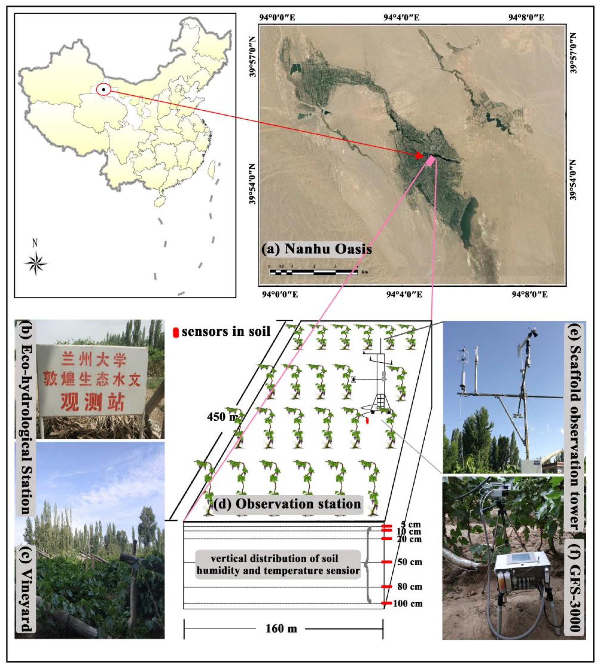
2.1. Site Description

The experiments were carried out in a sixteen-year-old grapevine plantation at the Dunhuang Eco-hydrological Station, located in the Nanhu Oasis, Gansu Province, northwest China (39°52’ N, 94°06’ E; 1300 m a.s.l). It is characterized by a typical temperate continental climate, with annual total radiation of 5903.4–6309.5 MW m−2 and an annual average temperature of 9.3 °C, respectively. The annual average precipitation is 36.9 mm, while the annual potential evapotranspiration reaches up to 2400 mm [23]. Nearly 80% of the precipitation falls between May and September. Grapevine is the most widely cultivated crop in this region because of its great economic and ecological value (Figure 1).
The selected plot measured 450 m × 160 m, in which Vitis vinifera L. (cv. Thompson Seedless) grapevines were planted. Here, Vitis vinifera L. arrayed with a spacing of 3 m, ensuring it received abundant radiation. The growing seasons begin in late April and end in the middle of October. The average canopy height is 1.5 m. Irrigation water is the main water source in this plot. The plot was furrow-irrigated about every 20 days during the growing seasons. Each irrigation event totaled approximately 142.5 mm, which can ensure an adequate water supply. According to the FAO classification, the soil type is Arenosols at the study site. Meanwhile, the mean soil bulk density is 1.41 g cm−3. An 18 m tall scaffold observation tower was installed in this plot for meteorological and eddy covariance measurements.

2.2. Experimental Design and Field Measurements

An automatic weather station (AWS-7500) provided continuous monitoring of meteorological factors during the growing seasons in 2016 and 2017. T (°C) and relative humidity (RH; %) (HMP60, Vaisala, Finland) were monitored by five-layer air temperature and humidity sensors (3, 2.5, 2, 1.5, and 1 m high above the ground, respectively). The volumetric soil water content (VWC; m3 m−3) (ML2x, Delta T, Cambridge, UK) was measured at depths of 100, 80, 50, 20, 10, and 5 cm. Wind speed (u; m s−1) (5103, R. M. Young, Traverse City, MI, USA) was measured 1.5 m above the canopy. The 30 min averages of observed data were recorded on a data logger (CR1000, Campbell, Logan, UT, USA). VPD (kPa) and PAR (μmol m−2 s−1) were also obtained from a portable gas exchange photosynthesis system (GFS-3000, Walz, Pfullingen, Germany). A tipping bucket rain gauge (TE525, Texas Electronics, Dallas, TX, USA) was installed in an open site about 500 m away from the tower to monitor the rainfall.
Gas exchange measurements were made from May to October in 2016 and 2017. Over the course of three typical sunny days in each month, Diurnal measurements from 6:00 to 22:00 (local time) of gs along with A (μmol m−2 s−1), transpiration (E; mmol m−2 s−1), and ambient (Ca) and leaf-internal (Ci) mole fractions of CO2 were made every 10 min on fully expanded mature leaves from sun-exposed terminal branches using the GFS-3000. Prior to gs measurements across diurnal courses, the airflow rate was set to 750 μmol s1, with an irradiance from the LED light source that followed ambient conditions. The cuvette temperature, humidity, and CO2 concentration were maintained as close as possible to the ambient environment.
Leaf water potential (Ψl) was measured using the Dewpoint PotentiaMeter from METER Group (WP4C Instruments, METER, Pullman, WA, USA). Pre-dawn leaf water potential (Ψl-pre) measurements were made prior to each diurnal measurement. After the gas exchange measurements, leaves were marked, and the diurnal course of Ψl was measured every 1 h from 8:00 to 20:00. Soil-to-leaf hydraulic conductance (KL) was defined as the volume flow rate divided by the difference of water potential across the flow path from soil to leaf [40]. It was estimated from average midday E inside the leaf chamber and the soil-leaf water potential difference (Ψs − Ψl). Usually, the soil water potential (Ψs) in the rooting zone was replaced by Ψl-pre, then KL was calculated as E/(Ψl-pre − Ψl).

2.3. Modeling Stomatal Conductance

An optimal stomatal conductance model derived from Medlyn et al. (2011) (hereafter, the USO model) was employed and has the following expression:
g s = g 0 + ( 1 + g 1 D ) A C a
where A is the net photosynthesis rate (μmol m−2 s−1), Ca represents ambient mole fractions of CO2 (ppm), D represents the vapor pressure deficit (kPa) at the leaf surface (the same as VPD). g0 represents the residual stomatal conductance as the net assimilation rate reaches zero. Generally, g0 is extremely small and assumed to be zero in many models [41]. g1 (kPa)0.5 is a fitted parameter called the stomatal conductance slope. In addition, the parameter g1 has a theoretical interpretation, as Medlyn et al. (2011) have shown:
g 1 = 3 Γ * 1.6 λ
g 1 Γ * λ
Γ * = Γ 25 * exp [ E Y ( T 298 ) 298 · R · T ]
That is, g1 is inversely proportional to the marginal water-use efficiency λ (mmol CO2 mol−1 H2O) and increases with the CO2 compensation point Γ*. Here, Γ*25 is the CO2 compensation point at 25 °C (3.74 Pa), EY represents the activation energy (26.80 kJ mol−1), and R is the universal gas constant (8.314 J mol−1 K−1). Model fitting and g1 estimations were conducted with Matlab 2015a software, using the Bayesian parameter estimation method [42].

3. Results

3.1. Environmental and Biological Variables

Daily variations of environmental conditions during the growing seasons in 2016 and 2017 are summarized in Figure 2. Inter-annual differences of the environmental factors were not obvious between the two study years. During the two study years, the highest air temperature (T) was 37.82, which occurred in July 2016 (at day of year 212, DOY 212 for short), and the lowest T, −3.01, occurred in October 2017 (at DOY 285). The mean air temperature during the growing seasons in 2016 and 2017 were 19.46 °C and 19.12 °C, respectively (Figure 2a,b). Generally, relative humidity (RH) was much lower in April and May than other months. The lowest RH was 0.16 in April 2016 (at DOY 119) and 0.12 in May 2017 (at DOY 127). The daily mean RH was around 0.45 (Figure 1c,d). The daily mean wind speed (u) ranged from 0.17 to 1.87 m s−1 (Figure 2c,d). The lowest u occurred in August and September of the two study years, while the highest u occurred in May and June, respectively. The daily mean vapor pressure deficit (VPD) ranged from 0.14 to 2.40 kPa, with a mean value of 1.27 kPa (Figure 2e,f). In general, daily mean photosynthesis active radiation (PAR) increased from spring, reaching its highest values in June and then declining from the end of June to a low value in October (Figure 2e,f). The peak values of the daily mean PAR in 2016 and 2017 were both reached in June, with a maximum value of 667.76 μmol m−2 s−1 (at DOY 163 in 2016) and 657.57 μmol m−2 s−1 (at DOY 172 in 2017), respectively. The variability of the volumetric soil water content (VWC) in different layers had similar trends, which were influenced by the irrigation schedule (Figure 2g,h). The variations of SWC were highly correlated with irrigation. The maximum of VWC was up to 0.31 m3 m-3 at depths of 50 cm in June 2016 (at DOY 166). The total amount of precipitation over the entire growing seasons was about 90.42 mm in 2016 and 27.18 mm in 2017 (Figure 2g,h). It is worth noting that the total precipitation in 2016 was much more than that in 2017. In 2016, most of the precipitation occurred in the middle of August (at DOY 230–234), which was associated with a single heavy rainfall event at DOY 230, which amounted to 52.07 mm in 24 h.

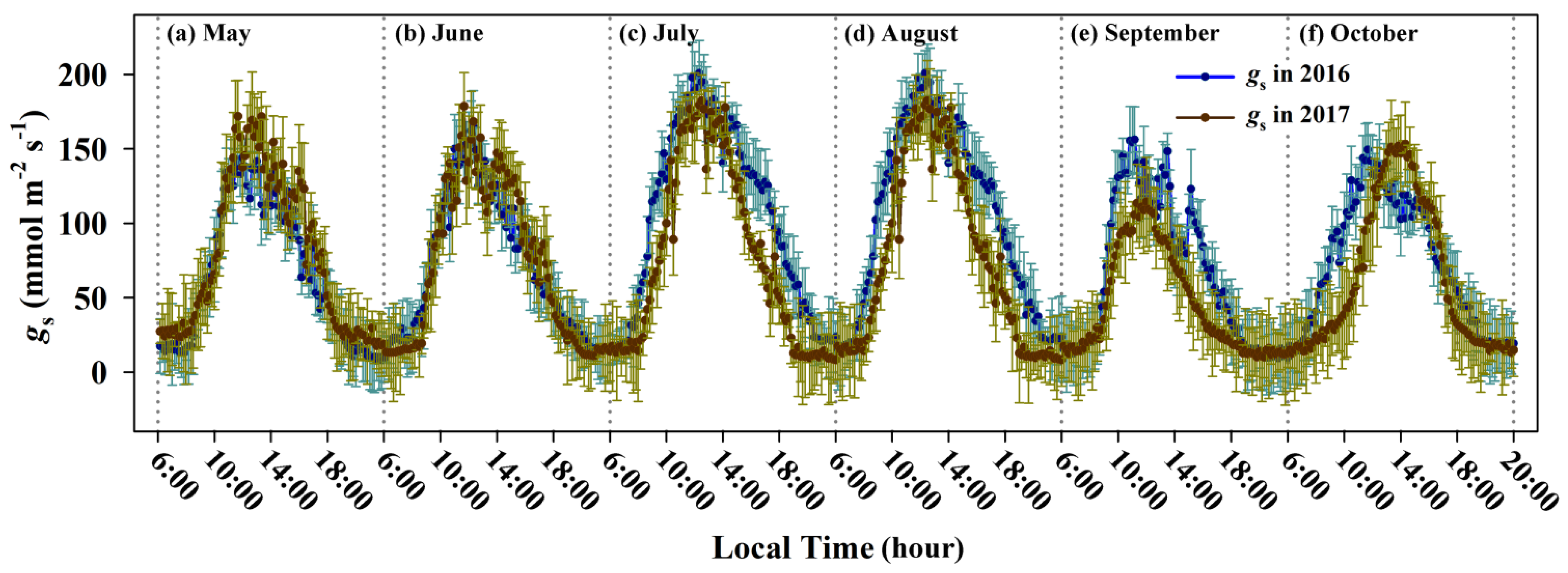
3.2. Diurnal Courses and Seasonal Variations of Stomatal Conductance

Diurnal courses of the observed gs over three consecutive sunny days each month during growing seasons are shown in Figure 3. Diurnal courses of gs demonstrated unimodal curves throughout the day, although slight fluctuations existed in some moments. This type of unimodal curve was observed throughout growing seasons and showed no significant inter-annual variations. Before sunrise, gs kept a relatively stable level, with mean values of 17.12 and 18.99 mmol m−2 s−1 in 2016 and 2017, respectively. After sunrise, with the increase in temperature and radiation, gs had a rapid increase between 8:00 and 11:00 local time. Peak values of gs mainly occurred mid-day (from about 12:00 to 14:00 in local time), with average values of 138.47, 140.51, 172.39, 168.45, 111.36, and 131.50 mmol m−2 s−1 in different months (from May to October, respectively). Then, gs declined gradually from 14:00 to 20:00. After sunset, gs dropped to a low value and remained stable.
Seasonal variations of gs were also compared in Figure 3. The trend of seasonal courses of gs showed a similar pattern for the two study years, which increased gradually from May, peaked in July, remained high until August, and then started declining. Maximum values in each month were both found in August, which were 211.68 mmol m−2 s−1 (DOY 238) and 185.64 mmol m−2 s−1 (DOY 235) in 2016 and 2007, respectively. Minimum values in each month were found in different months, which were 8.10 mmol m−2 s−1 (DOY 137) and 8.20 mmol m−2 s−1 (DOY 175) in 2016 and 2007, respectively. Notably, the mean value of gs in September 2017 (45.45 mmol m−2 s−1) seemed much lower than that in September 2016 (64.75 mmol m−2 s−1). This may be caused by a pruning event before harvest.

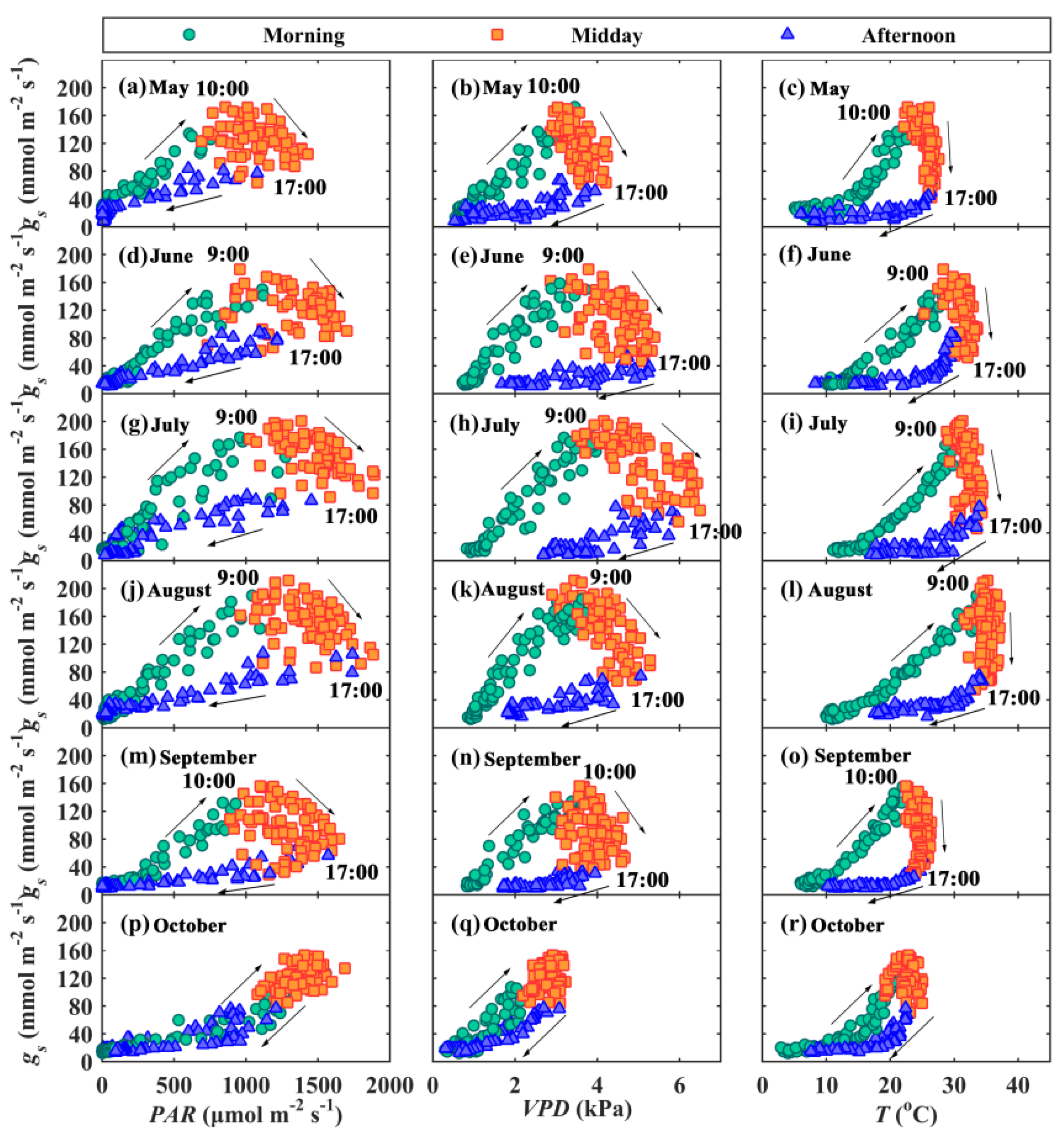
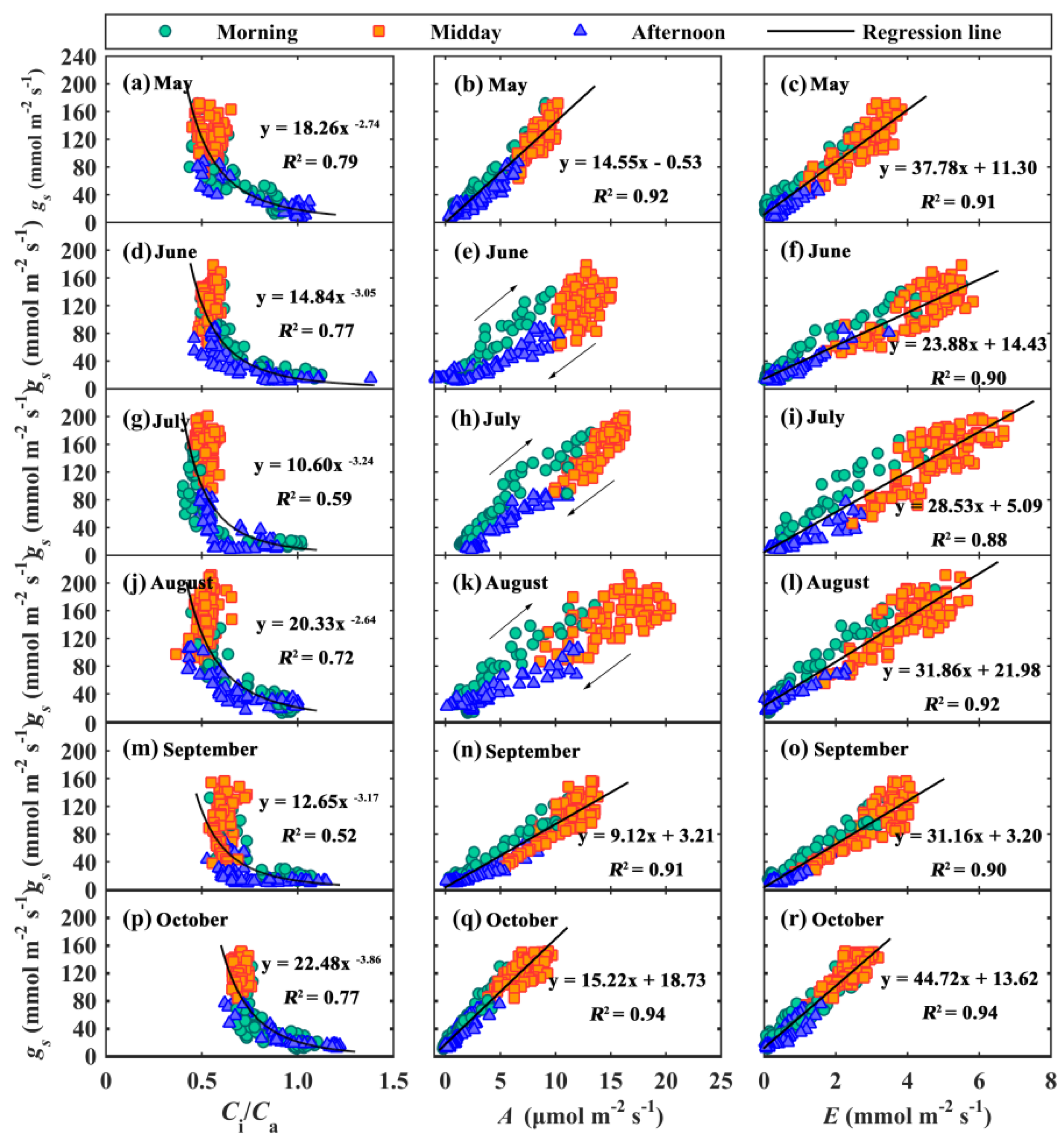
3.3. Hysteresis Loops between gs and Main Environmental and Biological Factors
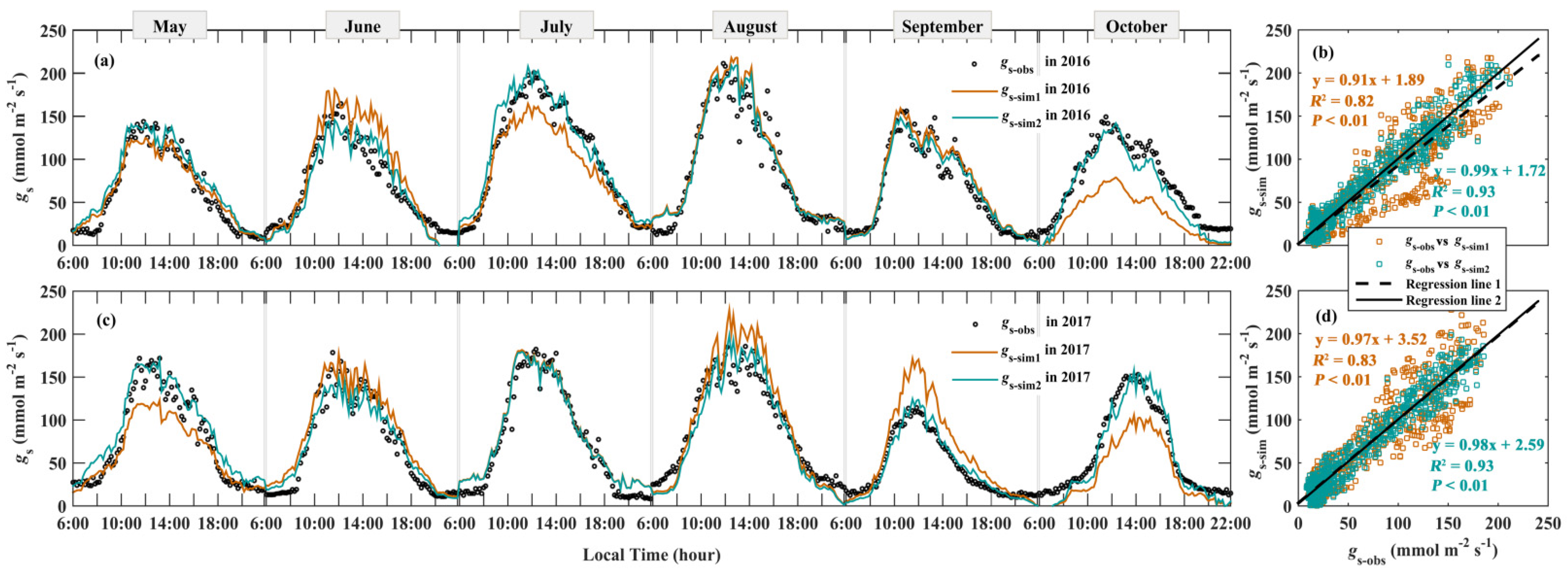
Hysteresis loops between gs and three main environmental factors (PAR, VPD, and T) were found throughout the day (Figure 4). The loop trajectory exhibited a clockwise direction following PAR, VPD, and T. Relationships between gs and environmental variables revealed different characteristics in three different daytime periods. Single-factor regressions between gs and PAR, VPD, and T in different time periods are presented in Table 1. In general, gs was positively correlated with PAR, VPD, and T in the morning period, changed to a negative correlation in the midday period, and became a positive correlation again in the afternoon. Furthermore, it was obvious that the hysteresis loops showed seasonal variation. That is, the turning points between the morning period and mid-day period were not always the same in each month. The turning points occurred around 10:00 at the beginning and end of the growing seasons (i.e., May, September, and October) and around 9:00 in June, July, and August. Additionally, peak values of gs in the loops exhibited differences in each month, ranging from about 150 mmol m−2 s−1 to 200 mmol m−2 s−1, with the maximum mid-day gs appearing in August (Figure 3). Otherwise, the hysteresis loops in October showed less regularities compared with the hysteresis loops in other months during the growing seasons, especially between gs and PAR.
Figure 5 showed the relationships between gs and three biological factors (Ci/Ca, A, and E). During a whole day, gs was negatively correlated with Ci/Ca. In the early morning, both gs and Ci/Ca kept a relatively stable level. With sunrise, gs increased gradually, while Ci/Ca dropped to a low value rapidly. After sunset, gs and Ci/Ca return to a stable state once again. The relationships between gs and A exhibited hysteresis loops in three months (from June to August) during growing seasons, which was relatively less obvious than hysteresis between gs and environmental variables. In May, August, and October, gs was linearly correlated with A (R2 = 0.92, 0.91, and 0.94, respectively; and slope = 14.55, 9.12, and 15.22, respectively). Moreover, gs and E were significantly linear related (Figure 5). The slopes of the linear regressions between gs and E ranged from 23.88 in June to 44.72 in October, with an average slope of 28.53 throughout the growing seasons.

3.4. Modeling gs

Figure 6 shows the posterior distributions for the parameter g1 in different months. The parameter representing stomatal conductance slope, g1, has been observed to change seasonally in this study. For example, median values of g1 in 2016 were lowest in June (2.47 kPa0.5), intermediate in July (4.50 kPa0.5), August (3.05 kPa0.5), September (3.14 kPa0.5), relatively larger in May (4.83 kPa0.5), and significantly larger in October (8.36 kPa0.5). In 2017, values of g1 mostly had similar variation across months as in 2016: they were relatively larger in May (4.83 kPa0.5) and October (6.05 kPa0.5), intermediate in June (2.79 kPa0.5), July (3.26 kPa0.5), August (2.73 kPa0.5), and lowest in September (1.92 kPa0.5). Overall, the median values of g1 in May and October were obviously higher than in the other months (Figure 6).
To evaluate the relationships between g1 and plant hydraulic conductance. Regression analysis between g1 and KL in different months was conducted (Table 1). g1 showed a significant linear positive correlation with KL across the entire growing seasons, with a slope and R2 of 0.18 and 0.95, respectively (Figure 7; p < 0.01).
Figure 8 visualizes the fits of the USO model to the datasets of diurnal courses in the growing seasons from May to October in 2016 (Figure 8a,b) and 2017 (Figure 8c,d), respectively. The fluctuations of observed and estimated diurnal gs are illustrated in Figure 6a,c. The model in which the seasonal variation of parameter g1 was taken into account (hereafter, the optimized USO model) had a big improvement in simulation accuracy in most months (e.g., July and October in 2016; May, August, and October in 2017). If the seasonal variation of parameter g1 was not considered, that is, using a fixed g1 value throughout the growing seasons (hereafter, the original USO model), overestimation and underestimation were prevalent in many months. To evaluate the performance of the optimized gs model for its application, we compared the simulated gs from the optimized (i.e., green diamonds) and original (i.e., brown diamonds) gs model to the observed datasets throughout the growing season in 2016 and 2017, respectively (Figure 8b,d). The slope of the regression of simulated versus observed values for the optimized USO model (0.99) was closer to 1 than that of the original USO model (0.91). Moreover, its R2 (0.93) was approximately 10% greater than that of the original USO model (0.82), indicating that the optimized USO model agreed better with the observed data (Figure 8b). Similarly, a better agreement between estimated and observed gs was obtained when using the optimized USO model compared to using the original USO model in 2017, with values of slopes equal to 0.98 and 0.97 and R2 equal to 0.93 and 0.83 (Figure 8d).

4. Discussion

4.1. Hysteresis Loops between gs and Its Influencing Factors

Environmental factors have long been found to have significant effects on stomatal conductance, which can largely affect the survival and development of a plant in competition [43,44]. Thus, relationships between gs and environmental variables have been widely discussed [45,46,47]. Previous studies have confirmed that plants adjusting their stomatal aperture to optimum are mainly affected by three environmental factors: PAR [48,49,50], VPD [51], and T [52], either alone and/or in combination. However, the relationships between gs and PAR, VPD, and T exhibited obvious inconsistency among diverse species, biomes, or even experimental methods and instruments. For example, Chang et al. (2006) reported that gs was exponentially negatively correlated with VPD [53], while Liu et al. (2015) found a positive linear relationship between them [22]. Relationships between gs and T are also varied. In recent years, a few diurnal hysteresis loops phenomena between stomatal conductance and these environmental factors were observed in some ecosystems and gradually attracted the attention of researchers [22,54]. Bai et al. (2015) also reported obvious hysteresis phenomena between gs at canopy level and global radiation, VPD, and T in a grape plantation in Nanhu oasis, an arid area of Northwest China [23]. However, the hysteretic loops phenomena of stomatal behavior were just identified at the canopy level in this study area. How exactly gs responses to these environmental factors, and if these hysteresis phenomena are also tenable in Nanhu oasis at leaf level have not been comprehensively documented.
In this study, the responses of gs to PAR, VPD, and T also formed obvious diurnal hysteresis loops and exhibited significantly seasonal variation (Figure 4). We had a hypothesis that the reported hysteresis phenomena involving gc at the canopy level may also be robust for gs at the leaf level, and this prediction was largely supported. In fact, the hysteresis loops during the daytime can be interpreted by the lags between gs and environmental variables during different time periods in a whole-day pattern. In the morning, stomata quickly opened combined with the increase in temperature and radiation. During this period of time, gs had significantly positive correlations with PAR, VPD, and T (with R2 > 0.70; Table 1). In the mid-day, temperature and radiation continued increasing and maintained a high level until afternoon, which induced stomatal closure to prevent excessive water loss in the form of transpiration [55]. Thus, gs decreased negatively with the increase in PAR, VPD, and T (Table 1). In the afternoon, stomata and these environmental factors kept decreasing simultaneously until sunset, gs once again positively correlated with PAR, VPD, and T (with R2 > 0.50; Table 1). In the desert oasis of arid northwest China, extremely high potential evapotranspiration and limited water availability make plants form a self-protective mechanism that the decline in the stomatal aperture was earlier than environmental factors to avoid too much water loss and then formed hysteresis loops between gs and these environmental factors. However, this time lag between gs and environmental factors was untenable in many previous studies [56], in which researchers mainly focused on mid-day datasets to characterize less-than-daily relationships between gs and environmental factors [21,57]. It implies that the proposed hysteresis loops are more credible in a whole-day pattern, especially in regions where water is scarce. Additionally, the turning points of the first two specific periods of time were not always the same in different months (Figure 4), which may be caused by the variability of the stomatal regulation during different growing stages of grapevines [58].

4.2. Seasonal Variations of g1

Stomatal behavior responding to environmental variables is a key module in LSMs under current climate change scenarios [59]. Although there has been considerable ongoing model development to implement stomatal conductance estimation into LSMs, an associated globally applicable gs model that has a strong grounding in physiological theory is required [2,60]. In recent years, the optimal stomatal conductance model (e.g., the USO model), which is derived from leaf-level physiological theory and has the ability to predict how gs response to changing environments in the future, such as warmer temperature, elevated CO2 concentration, and shortage of water availability has been encouraged to use in LSMs [6,10,61]. The USO model is attractive because, unlike empirical models, it provides a meaningful slope parameter g1 that is closely related to the marginal carbon cost of water use (λ). Exploring variations of g1 in different conditions would help to interpret a plant’s water-use strategy in terms of the trade-off between carbon gain and water loss. As a baseline for accurately simulating gs variations, we should acknowledge that the USO model does not allow us to use a completely universal g1 value in different climatic conditions, biomes, and PFTs. Medlyn et al. (2011) confirmed that parameter g1 varied with PFTs, with the lowest values in gymnosperms and conifers and the highest in deciduous angiosperms. Lin et al. (2015) presented distributions of g1 in a broader range of PFTs and biomes and confirmed that g1 values varied several folds across different PFTs and were positively related with climate variables (i.e., temperature and moisture index).
We had hypothesized that g1 values would vary in different growing seasons. This hypothesis was largely supported, as we found a clear pattern of g1 variation among growing seasons (Figure 6). Additionally, it can be supported by plant hydraulic conductance, i.e., g1 showed a significant positive correlation with KL across the entire growing seasons (Figure 7; p < 0.01). The observed variations of KL functions and thus water-use strategies across seasons showed that: during the early and late development stage (local time in May and October), a high value of KL represents water that is much easier to escape from the soil to the atmosphere through vessels in the root, stems, and leaves, meaning that grapevines have a costly water-use strategy, then a high g1 (small λ); while in the main growing seasons (local time from June to September), grapevines have a conservative water-use strategy (i.e., a small value of g1 and high λ), which is advantageous for matter accumulation. This result has been supported by many previous studies that multiple strategies involving a series of plan biological traits, for instance, xylem hydraulic conductivity, leaf area, soil water content, and wood density, are possible throughout the growing seasons [40,62]. Furthermore, it suggested that the current use of g1 in LSMs may be missing an important element of seasonal variations. Although there has been a lot of research on how g1 varies among species, PFTs, and biomes, challenges still remain in providing a more robust parameter input for future simulation of LSMs in different phenological periods. This research offers new insight into the quantitative analysis parameter g1, which further helps to explore dynamic water-use strategies of plants in different growing seasons.

4.3. Looking Forward

Stomatal conductance, gs, plays a pivotal role in LSMs as it controls the exchange of carbon, water, and energy between the lower atmosphere and the terrestrial biosphere. Exploring stomatal behavior and accurately estimating gs are very important to understanding the carbon–water cycles of terrestrial ecosystems. The gas exchange system provides a powerful tool to obtain continuous and instantaneous gs information and thus has great potential in modeling the spatial dynamics of gs over broad regions. Thus, it has been adequately confirmed in previous studies on parameter fitting that the stomatal conductance slope g1 is specified by diverse PFTs and climatic conditions. In fact, as this study confirmed, g1 tends to vary throughout the growing seasons, even for a certain species. Therefore, more work to analyze the spatial dynamics of g1 is required in the future.
Along with the climate change accelerating, it is more urgent now than ever for us to develop and optimize models to predict the future. Currently, parameter values or correlations between variables obtained at one scale were often assumed to be relatable to other scales. However, our comparison indicates that the proposed hysteresis loops between gs and environmental factors can be established in a whole-day pattern rather than a less-than-daily pattern. Hence, there is a need for us to notice the potential bias when using some inherent relationships to constrain LSMs.

5. Conclusions

We combined gas exchange measurements with an optimal stomatal conductance model simulation to explore diurnal and seasonal variability of gs in different growing seasons for a vineyard at Nanhu oasis, Northwest China. First, in agreement with our hypothesis, stomata and environmental factors (PAR, VPD, and T) exhibited obvious hysteresis loops at the leaf level throughout the day. Second, the stomatal conductance slope g1 exhibited obvious seasonal variation. Additionally, g1 was significantly positively correlated with KL, which implied a different water-use strategy over the course of the growing seasons. Last, the optimized USO model (i.e., seasonal variation of parameter g1 was considered) has a big improvement in estimation accuracy than the original USO model (i.e., using a completely universal g1 value). This study reconstructed our knowledge of relationships between gs and environmental variables and the seasonal variation of the water-use strategy in the desert oasis of an arid area in northwestern China. Future studies should pay more attention to seasonal dynamics of g1 values by relating them to different growing stages, as it may help to precisely interpret the carbon–water cycle in LSMs.

Author Contributions

Conceptualization, methodology, supervision, and funding acquisition Q.F.; methodology, investigation, resources, data curation, writing—original draft, and writing—review and editing, T.H.; validation, T.Y.; visualization, X.Y., X.Z. and K.L. All authors have read and agreed to the published version of the manuscript.

Funding

This research was funded by the National Natural Science Fund of China, grant number 52179026, 41771252; the Forestry and Grassland Science and Technology Innovation Program of Gansu Province, grant number GYCX [2020]01; the Key R&D Program of Gansu Province, China, grant number 20YF8FA002; the XPCC Science and Technique Foundation, grant number 2021AB021; the Think Tank Platform Construction Program of Gansu Association for Science and Technology, grant number GSAST-ZKPT [2020]01; and the Major Research Program of Inner Mongolia, grant number zdzx2018057.

Institutional Review Board Statement

Not applicable.

Informed Consent Statement

Not applicable.

Data Availability Statement

The source of relevant data acquisition has been described in the text.

Acknowledgments

We acknowledge support from the Key Laboratory of Western China’s Environmental Systems (Ministry of Education), Lanzhou University.

Conflicts of Interest

The authors declare no conflict of interest.

References

  1. Lin, Y.S.; Medlyn, B.E.; Duursma, R.A.; Prentice, I.C.; Wang, H.; Baig, S.; Eamus, D.; de Dios, V.R.; Mitchell, P.; Ellsworth, D.S.; et al. Optimal stomatal behaviour around the world. Nat. Clim. Chang. 2015, 5, 459–464. [Google Scholar] [CrossRef] [Green Version]
  2. Franks, P.J.; Bonan, G.B.; Berry, J.A.; Lombardozzi, D.L.; Holbrook, N.M.; Herold, N.; Oleson, K.W. Comparing optimal and empirical stomatal conductance models for application in Earth system models. Glob. Chang. Biol. 2018, 24, 5708–5723. [Google Scholar] [CrossRef] [PubMed]
  3. Berry, J.A.; Beerling, D.J.; Franks, P.J. Stomata: Key players in the earth system, past and present. Curr. Opin. Plant Biol. 2010, 13, 232–239. [Google Scholar] [CrossRef] [PubMed]
  4. Dewar, R.C. The Ball-Berry-Leuning and Tardieu-Davies stomatal models: Synthesis and extension within a spatially aggregated picture of guard cell function. Plant Cell Environ. 2002, 25, 1383–1398. [Google Scholar] [CrossRef]
  5. Ahsan, A.; Yaseen, A.A.; Yassine, C.; Ghazi, A.R.; Malik, A. Satellite-Based Water and Energy Balance Model for the Arid Region to Determine Evapotranspiration: Development and Application. Sustainability 2021, 13, 13111. [Google Scholar] [CrossRef]
  6. Bonan, G.B.; Williams, M.; Fisher, R.A.; Oleson, K.W. Modeling stomatal conductance in the earth system: Linking leaf water-use efficiency and water transport along the soil–plant–atmosphere continuum. Geosci. Model Dev. 2014, 7, 2193–2222. [Google Scholar] [CrossRef] [Green Version]
  7. Zhu, Z.; Piao, S.; Myneni, R.B.; Huang, M.; Zeng, Z.; Canadell, J.G.; Ciais, P.; Sitch, S.; Friedlingstein, P.; Arneth, A.; et al. Greening of the Earth and its drivers. Nat. Clim. Chang. 2016, 6, 791–795. [Google Scholar] [CrossRef]
  8. Miner, G.L.; Bauerle, W.L.; Baldocchi, D.D. Estimating the sensitivity of stomatal conductance to photosynthesis: A review. Plant Cell Environ. 2017, 40, 1214–1238. [Google Scholar] [CrossRef]
  9. Franks, P.J.; Berry, J.A.; Lombardozzi, D.L.; Bonan, G.B. Stomatal Function across Temporal and Spatial Scales: Deep-Time Trends, Land-Atmosphere Coupling and Global Models. Plant Physiol. 2017, 174, 583–602. [Google Scholar] [CrossRef] [Green Version]
  10. Medlyn, B.E.; De Kauwe, M.G.; Lin, Y.S.; Knauer, J.; Duursma, R.A.; Williams, C.A.; Arneth, A.; Clement, R.; Isaac, P.; Limousin, J.M.; et al. How do leaf and ecosystem measures of water-use efficiency compare? New Phytol. 2017, 216, 758–770. [Google Scholar] [CrossRef] [Green Version]
  11. Ogle, K.; Reynolds, J.F. Desert dogma revisited: Coupling of stomatal conductance and photosynthesis in the desert shrub, Larrea tridentata. Plant Cell Environ. 2002, 25, 909–921. [Google Scholar] [CrossRef]
  12. Héroult, A.; Lin, Y.S.; Bourne, A.; Medlyn, B.E.; Ellsworth, D.S. Optimal stomatal conductance in relation to photosynthesis in climatically contrasting Eucalyptus species under drought. Plant Cell Environ. 2013, 36, 262–274. [Google Scholar] [CrossRef]
  13. Limousin, J.M.; Bickford, C.P.; Dickman, L.T.; Pangle, R.E.; Hudson, P.J.; Boutz, A.L.; Gehres, N.; Osuna, G.J.; Pockman, W.T.; Mcdowell, N.G. Regulation and acclimation of leaf gas exchange in a piñon–juniper woodland exposed to three different precipitation regimes. Plant Cell Environ. 2013, 36, 1812–1825. [Google Scholar] [CrossRef] [Green Version]
  14. Sitch, S.; Smith, B.; Prentice, I.C.; Arneth, A.; Bondeau, A.; Cramer, W.; Kaplan, J.O.; Levis, S.; Lucht, W.; Sykes, M.T.; et al. Evaluation of ecosystem dynamics, plant geography and terrestrial carbon cycling in the LPJ dynamic global vegetation model. Glob. Chang. Biol. 2003, 9, 161–185. [Google Scholar] [CrossRef]
  15. Massman, W.J.; Kaufmann, M.R. Stomatal response to certain environmental factors: A comparison of models for subalpine trees in the Rocky Mountains. Agric. For. Meteorol. 1991, 54, 155–167. [Google Scholar] [CrossRef]
  16. Buckley, T.N.; Mott, K.A. Modelling stomatal conductance in response to environmental factors. Plant Cell Environ. 2013, 36, 1691–1699. [Google Scholar] [CrossRef] [PubMed]
  17. Jiao, L.; Wang, L.H.; Zhou, Q.; Huang, X.H. Stomatal and non-stomatal factors regulated the photosynthesis of soybean seedlings in the present of exogenous bisphenol A. Ecotoxicol. Environ. Saf. 2017, 145, 150–160. [Google Scholar] [CrossRef] [PubMed]
  18. Sulman, B.N.; Roman, D.T.; Yi, K.; Wang, L.X.; Phillips, R.P.; Novick, K.A. High atmospheric demand for water can limit forest carbon uptake and transpiration as severely as dry soil. Geophys. Res. Lett. 2016, 43, 9686–9695. [Google Scholar] [CrossRef]
  19. Lin, C.J.; Gentine, P.; Huang, Y.F.; Guan, K.Y.; Kimm, H.; Zhou, S. Diel ecosystem conductance response to vapor pressure deficit is suboptimal and independent of soil moisture. Agric. For. Meteorol. 2018, 250–251, 21–34. [Google Scholar] [CrossRef]
  20. Tang, J.; Bolstad, P.V.; Ewers, B.E.; Desai, A.R.; Davis, K.J.; Carey, E.V. Sap flux-upscaled canopy transpiration, stomatal conductance, and water use efficiency in an old growth forest in the Great Lakes region of the United States. J. Geophys. Res. 2006, 111, G02009. [Google Scholar] [CrossRef] [Green Version]
  21. Igarashi, Y.; Kumagai, T.O.; Yoshifuji, N.; Sato, T.; Tanaka, N.; Tanaka, K.; Suzuki, M.; Tantasirin, C. Environmental control of canopy stomatal conductance in a tropical deciduous forest in northern Thailand. Agric. For. Meteorol. 2015, 202, 1–10. [Google Scholar] [CrossRef]
  22. Liu, H.; Cohen, S.; Lemcoff, J.H.; Israeli, Y.; Tanny, J. Sap flow, canopy conductance and microclimate in a banana screenhouse. Agric. For. Meteorol. 2015, 201, 165–175. [Google Scholar] [CrossRef]
  23. Bai, Y.; Zhu, G.F.; Su, Y.H.; Zhang, K.; Han, T.; Ma, J.Z.; Wang, W.Z.; Ma, T.; Feng, L.L. Hysteresis loops between canopy conductance of grapevines and meteorological variables in an oasis ecosystem. Agric. For. Meteorol. 2015, 214–215, 319–327. [Google Scholar] [CrossRef]
  24. Bai, Y.; Li, X.Y.; Liu, S.M.; Wang, P. Modelling diurnal and seasonal hysteresis phenomena of canopy conductance in an oasis forest ecosystem. Agric. For. Meteorol. 2017, 246, 98–110. [Google Scholar] [CrossRef]
  25. Jarvis, P.G. The interpretation of the variations in leaf water potential and stomatal conductance found in canopies in the field. Philos. Trans. R. Soc. Lond. Ser. B 1976, 273, 593–610. [Google Scholar] [CrossRef]
  26. Ball, M.C.; Woodrow, I.E.; Berry, J.A. A model predicting stomatal conductance and its contribution to the control of photosynthesis under different environmental conditions. In Progress in Photosynthesis Research; Biggins, J., Ed.; Martinus Nijhoff Publishers: Dordrecht, The Netherlands, 1987; pp. 221–224. [Google Scholar] [CrossRef]
  27. Leuning, R. Modelling stomatal behaviour and photosynthesis of Eucalyptus grandis. Aust. J. Plant Physiol. 1990, 17, 159–175. [Google Scholar] [CrossRef]
  28. Monteith, J.L. A reinterpretation of stomatal responses to humidity. Plant Cell Environ. 1995, 18, 357–364. [Google Scholar] [CrossRef]
  29. Cowan, I.R. Oscillations in stomatal conductance and plant functioning associated with stomatal conductance: Observations and a model. Planta 1972, 106, 185–219. [Google Scholar] [CrossRef] [PubMed]
  30. Hills, A.; Chen, Z.H.; Amtmann, A.; Blatt, M.R.; Lew, V.L. OnGuard, a computational platform for quantitative kinetic modeling of guard cell physiology. Tree Physiol. 2012, 159, 1026–1042. [Google Scholar] [CrossRef] [PubMed] [Green Version]
  31. Prentice, I.C.; Dong, N.; Gleason, S.M.; Maire, V.; Wright, I.J. Balancing the costs of carbon gain and water transport: Testing a new theoretical framework for plant functional ecology. Ecol. Lett. 2014, 17, 82–91. [Google Scholar] [CrossRef] [PubMed]
  32. Sellers, P.J.; Randall, D.A.; Collatz, G.J.; Berry, J.A.; Field, C.B.; Dazlich, D.A.; Zhang, C.; Collelo, G.D.; Bounoua, L. A revised land surface parameterization (SiB2) for atmospheric GCMs. Part 1: Model formulation. J. Clim. 1996, 9, 676–705. [Google Scholar] [CrossRef]
  33. Bonan, G.B.; Doney, S.C. Limate, ecosystems, and planetary futures: The challenge to predict life in Earth system models. Science 2018, 359, eaam8328. [Google Scholar] [CrossRef] [PubMed] [Green Version]
  34. Cowan, I.R.; Farquhar, G.D. Stomatal function in relation to leaf metabolism and environment. In Integration of Activity in the Higher Plant; Jennings, D.H., Ed.; Cambridge University Press: Cambridge, UK, 1977; pp. 471–505. [Google Scholar] [CrossRef]
  35. Knauer, J.; Zaehle, S.; Medlyn, B.E.; Reichstein, M.; Williams, C.A.; Migliavacca, M.; De Kauwe, M.G.; Werner, C.; Keitel, C.; Kolari, P.; et al. Towards physiologically meaningful water-use efficiency estimates from eddy covariance data. Glob. Chang. Biol. 2018, 24, 694–710. [Google Scholar] [CrossRef] [PubMed]
  36. Sinclair, T.R.; Tanner, C.B.; Bennett, J.M. Water-use efficiency in crop production. BioScience 1984, 34, 36–40. [Google Scholar] [CrossRef]
  37. Ye, Z.; Fu, A.; Zhang, S.; Yang, Y. Suitable scale of an oasis in different scenarios in an arid region of china: A case study of the ejina oasis. Sustainability 2020, 12, 2583. [Google Scholar] [CrossRef] [Green Version]
  38. Zhao, L.; Li, W.; Yang, G.; Yan, K.; He, X.; Li, F.; Gao, Y.; Tian, L. Moisture, temperature, and salinity of a typical desert plant (Haloxylon ammodendron) in an arid oasis of northwest china. Sustainability 2021, 13, 1908. [Google Scholar] [CrossRef]
  39. Zhang, Q.; Huang, R.H. Water vapor exchange between soil and atmosphere over a Gobi surface near an oasis in Summer. J. Appl. Meteorol. 2004, 43, 1917–1928. [Google Scholar] [CrossRef]
  40. Sperry, J.S.; Meinzer, F.C.; McCulloh, K.A. Safety and efficiency conflicts in hydraulic architecture: Scaling from tissues to trees. Plant Cell Environ. 2008, 31, 632–645. [Google Scholar] [CrossRef] [PubMed]
  41. De Kauwe, M.G.; Medlyn, B.E.; Zaehle, S.; Walker, A.P.; Dietzem, C.; Hickler, T.; Jain, A.K.; Luo, Y.Q.; Parton, W.J.; Prentice, I.C.; et al. Forest water use and water use efficiency at elevated CO2: A model-data intercomparison at two contrasting temperate forest FACE sites. Glob. Chang. Biol. 2013, 19, 1759–1779. [Google Scholar] [CrossRef]
  42. Zhu, G.F.; Li, X.; Zhang, K.; Ding, Z.Y.; Han, T.; Ma, J.Z.; Huang, C.L.; He, J.H.; Ma, T. Multi-model ensemble prediction of terrestrial evapotranspiration across north China using Bayesian model averaging. Hydrol. Process. 2016, 30, 2861–2879. [Google Scholar] [CrossRef]
  43. Merilo, E.; Jõesaar, I.; Brosché, M.; Kollist, H. To open or to close: Species-specific stomatal responses to simultaneously applied opposing environmental factors. New Phytol. 2014, 202, 499–508. [Google Scholar] [CrossRef] [PubMed]
  44. Kołodziejek, J. Growth and competitive interaction between seedlings of an invasive Rumex confertus and of cooccurring two native Rumex species in relation to nutrient availability. Nature 2019, 9, 3298. [Google Scholar] [CrossRef] [Green Version]
  45. Song, X.; Zhou, G.; He, Q. Critical leaf water content for maize photosynthesis under drought stress and its response to rewatering. Sustainability 2021, 13, 7218. [Google Scholar] [CrossRef]
  46. Ono, K.; Maruyama, A.; Kuwagata, T.; Mano, M.; Takimoto, T.; Hayashi, K.; Hasegawa, T.; Miyata, A. Canopy-scale relationships between stomatal conductance and photosynthesis in irrigated rice. Glob. Chang. Biol. 2013, 19, 2209–2220. [Google Scholar] [CrossRef]
  47. Yan, W.M.; Zhong, Y.Q.W.; Shangguan, Z.P. Contrasting responses of leaf stomatal characteristics to climate change: A considerable challenge to predict carbon and water cycles. Glob. Chang. Biol. 2017, 23, 3781–3793. [Google Scholar] [CrossRef] [PubMed]
  48. Scafaro, A.P.; Xiang, S.; Long, B.M.; Bahar, N.A.; Weerasinghe, L.K.; Creek, D.; Evans, J.R.; Reith, P.B.; Atkin, O.K. Strong thermal acclimation of photosynthesis in tropical and temperate wet-forest tree species: The importance of altered Rubisco content. Glob. Chang. Biol. 2017, 23, 2783–2800. [Google Scholar] [CrossRef]
  49. Wu, C.; Wang, X.; Wang, H.; Ciais, P.; Peñuelas, J.; Myneni, R.B.; Desai, A.R.; Gough, C.M.; Gonsamo, A.; Black, A.T.; et al. Contrasting resp-onses of autumn-leaf senescence to daytime and night-time warming. Nat. Clim. Chang. 2018, 8, 1092–1096. [Google Scholar] [CrossRef] [Green Version]
  50. Drake, J.E.; Tjoelker, M.G.; Vårhammar, A.; Medlyn, B.E.; Reich, P.B.; Leigh, A.; Pfautsch, S.; Blackman, C.J.; López, R.; Aspinwall, M.J.; et al. Trees tolerate an extreme heatwave via sustained transpirational cooling and increased leaf thermal tolerance. Glob. Chang. Biol. 2018, 24, 2390–2402. [Google Scholar] [CrossRef] [PubMed]
  51. Marchin, R.M.; Broadhead, A.A.; Bostic, L.E.; Dunn, R.R.; Hoffmann, W.A. Stomatal acclimation to vapor pressure d-eficit doubles transpiration of small tree seedlings with warming. Plant Cell Environ. 2016, 39, 2221–2234. [Google Scholar] [CrossRef] [PubMed]
  52. Duursma, R.A.; Barton, C.V.M.; Lin, Y.S.; Medlyn, B.E.; Eamus, D.; Tissue, D.T.; Ellsworth, D.S.; McMurtrie, R.E. The peaked response of transpiration rate to vapour pressure deficit in field conditions can be explained by the temperature optimum of photosynthesis. Agric. For. Meteorol. 2014, 189, 2–10. [Google Scholar] [CrossRef] [Green Version]
  53. Chang, X.; Zhao, W.; Zhang, Z.; Su, Y. Sap flow and tree conductance of shelter-belt in arid region of China. Agric. For. Meteorol. 2006, 138, 132–141. [Google Scholar] [CrossRef]
  54. Jones, H.G. Plant and Microclimate: A Quantitative Approach to Environmental Plant Physiology, 3rd ed.; Cambridge University Press: Cambridge, UK, 2014; pp. 135–144. [Google Scholar] [CrossRef]
  55. Wang, S.T.; Zhu, G.F.; Xia, D.S.; Ma, J.Z.; Han, T.; Ma, T.; Zhang, K.; Shang, S.S. The characteristics of evapotranspiration and crop coefficients of an irrigated vineyard in arid Northwest China. Agric. Water Manag. 2019, 212, 388–398. [Google Scholar] [CrossRef]
  56. Rodrigues, T.R.; Vourlitis, G.L.; Lobo, F.D.A.; Santanna, F.B.; Arruda, P.H.Z.D.; Nogueira, J.D.S. Modeling canopy conductance under contrasting seasonal conditions for a tropical savanna ecosystem of south central Mato Grosso, Brazil. Agric. For. Meteorol. 2016, 23, 218–229. [Google Scholar] [CrossRef] [Green Version]
  57. Tie, Q.; Hua, H.C.; Tian, F.Q.; Guan, H.D.; Lin, H. Environmental and physiological controls on sap flow in a subh-umid mountainous catchment in North China. Agric. For. Meteorol. 2017, 240–241, 46–57. [Google Scholar] [CrossRef]
  58. Aasamaa, K.; Sõber, A. Stomatal sensitivities to changes in leaf water potential, air humidity, CO2 concentration and light intensity, and the effect of abscisic acid on the sensitivities in six temperate deciduous tree species. Environ. Exp. Bot. 2011, 71, 72–78. [Google Scholar] [CrossRef]
  59. Song, Q.H.; Fei, X.H.; Zhang, Y.P.; Sha, L.Q.; Liu, Y.T.; Zhou, W.J.; Wu, C.S.; Lu, Z.Y.; Luo, K.; Gao, J.B.; et al. Water use efficiency in a primary subtropical evergreen forest in Southwest China. Sci. Rep. 2017, 7, 43031. [Google Scholar] [CrossRef] [PubMed] [Green Version]
  60. De Kauwe, M.G.; Kala, J.; Lin, Y.S.; Pitman, A.J.; Medlyn, B.E.; Duursma, R.A.; Abramowitz, G.; Wang, Y.P.; Miralles, D.G. A test of an optimal stomatal conductance scheme within the CABLE land surface model. Geosci. Model Dev. 2015, 8, 431–452. [Google Scholar] [CrossRef] [Green Version]
  61. Li, X.; Xiao, J.; He, B.; Arain, M.A.; Beringer, J.; Desai, A.R.; Emmel, C.; Hollinger, D.Y.; Krasnova, A.; Mammarella, I.; et al. Solar-induced chlorophyll fluorescence is strongly correlated with terrestrial photosynthesis for a wide variety of biomes: First global analysis based on OCO-2 and flux tower observations. Glob. Chang. Biol. 2018, 24, 3990–4008. [Google Scholar] [CrossRef] [PubMed]
  62. Anderegg, W.R.L.; Wolf, A.; Arango-Velez, A.; Choat, B.; Chmura, D.J.; Jansen, S.; Kolb, T.; Li, S.; Meinzer, F.C.; Pita, P.; et al. Woody plants optimise stomatal behaviour relative to hydraulic risk. Ecol. Lett. 2018, 21, 968–977. [Google Scholar] [CrossRef] [PubMed] [Green Version]
Figure 1. (a) Location of the study area in Nanhu Oasis, Gansu Province, northwestern China. (b) Dunhuang Ecohydrological Station. (c) Image of the vineyard and underlying surface. (d) Diagram of the observation station. (e) Scaffold observation tower used for both meteorological measurements and eddy covariance. (f) Portable gas exchange fluorescence system (GFS-3000).
Sustainability 14 00968 g001
Figure 2. Environmental factors during the study periods 2016 and 2017, including (a,b) daily minimum/maximum and mean air temperature (T, °C), (c,d) daily mean relative humidity (RH), daily mean wind speed (u, m s−1), (e,f) daily mean vapor pressure deficit (VPD, kPa), daily photosynthetically active radiation (PAR, μmol m−2 s−1), (g,h) daily soil water content (VWC, m3 m3) at 5, 10, 20, 50, 80, and 100 cm depth, daily precipitation (P, mm), and irrigation (cm). “DOY” in the horizontal axis means day of year.
Sustainability 14 00968 g002
Figure 3. Diurnal courses of stomatal conductance (gs, mmol m−2 s−1) in three sunny days from May to October in 2016 and 2007, respectively. (af) represent datasets from May to October, respectively. The bars represent the standard deviations of the mean.
Sustainability 14 00968 g003
Figure 4. Hysteresis loops between stomatal conductance (gs, mmol m−2 s−1) and the main micrometeorological variables, i.e., (a,d,g,j,m,p) photosynthetically active radiation (PAR, μmol m−2 s−1), (b,e,h,k,n,q) mean vapor pressure deficit (VPD, kPa), and (c,f,i,l,o,r) air temperature (T, °C) during the diurnal cycle of the recently fully expanded leaves from May to October.
Sustainability 14 00968 g004
Figure 5. Correlations between stomatal conductance (gs, mmol m2 s1) and the main bio-chemical variables, i.e., (a,d,g,j,m,p) intercellular CO2 concentration to ambient CO2 concentration (Ci/Ca,), (b,e,h,k,n,q) net photosynthesis rate (A, μmol m2 s1), and (c,f,i,l,o,r) transpiration rate (E, μmol m2 s1) during the diurnal cycle of the recently fully expanded leaves from May to October.
Sustainability 14 00968 g005
Figure 6. Stomatal conductance slope (g1) varies in different growing seasons (from May to October) in 2016 (a) and 2017 (b), respectively. Boxes mark the 75th and 25th percentiles, and the dashed and solid lines in the boxes refer to the average and median values, respectively.
Sustainability 14 00968 g006
Figure 7. Correlations between g1 and KL. Boxes mark the 75th and 25th percentiles, and the dashed and solid lines in the boxes refer to the average and median values, respectively.
Sustainability 14 00968 g007
Figure 8. Comparison between the observed and simulated stomatal conductance (gs-obs, mmol m−2 s−1 and gs-sim, mmol m−2 s−1) in 2016 (a,b) and 2017 (c,d), respectively. Green lines represent the simulated gs in using optimized USO model; the brown lines represent the simulated gs in using original USO model.
Sustainability 14 00968 g008
Table 1. Single-factor regressions between stomatal conductance (gs) and photosynthesis active radiation (PAR), vapor pressure deficit (VPD), and air temperature (T) in different time periods of the day in each month of the growing season, R2 is the coefficient of determination.
MonthFactorMorningMiddayAfternoon
Regression LineR2Regression LineR2Regression LineR2
MayPARgs = 0.15 × PAR + 22.720.94gs = −0.04 × PAR + 175.250.10gs = 0.06 × PAR + 18.910.89
VPDgs = 46.01 × VPD − 10.680.91gs = −37.91 × VPD + 258.420.33gs = 9.19 × e0.49VPD0.69
Tgs = 6.03 × T − 29.630.76gs = −11.45 × T + 418.740.40gs = 5.54 × e0.08T0.60
JunPARgs = 0.15 × PAR + 8.790.92gs = −0.04 × PAR + 183.360.17gs = 0.06 × PAR + 12.920.90
VPDgs = 56.68 × VPD − 29.630.87gs = −17.61 × VPD + 202.820.26gs = 6.42 × e0.42VPD0.54
Tgs = 7.04 × T − 70.790.90gs = −5.42 × T + 296.240.19gs = 4.35 × e0.08T0.73
JulPARgs = 0.14 × PAR + 17.410.76gs = −0.02 × PAR + 176.020.02gs = 0.07 × PAR + 12.680.87
VPDgs = 50.66 × VPD − 33.760.90gs = −18.11 × VPD + 236.090.23gs = 2.18 × e0.59VPD0.74
Tgs = 7.14 × T − 78.970.91gs = −18.97 × T + 758.690.56gs = 1.04 × e0.12T0.64
AugPARgs = 0.15 × PAR + 19.090.93gs = −0.05 × PAR + 217.400.12gs = 0.04 × PAR + 23.600.88
VPDgs = 49.42 × VPD − 46.360.89gs = −24.43 × VPD + 246.480.28gs = 11.75 × e0.37VPD0.72
Tgs = 6.05 × T − 53.410.94gs = −1.88 × T + 215.870.01gs = 5.41 × e0.07T0.72
SepPARgs = 0.12 × PAR + 5.640.94gs = −0.02 × PAR + 113.270.01gs = 0.03 × PAR + 10.050.81
VPDgs = 48.43 × VPD − 27.720.95gs = −11.93 × VPD + 136.540.03gs = 3.53 × e0.57VPD0.70
Tgs = 8.19 × T − 47.950.94gs = −3.05 × T + 166.360.01gs = 3.60 × e0.09T0.69
OctPARgs = 16.45 × e0.0014PAR0.94--gs = 16.01 × e0.0013PAR0.79
VPDgs = 11.58 × e0.92VPD0.83--gs = 11.43 × e0.70VPD0.92
Tgs = 8.88 × e0.12T0.94--gs = 5.66 × e0.10T0.72
Publisher’s Note: MDPI stays neutral with regard to jurisdictional claims in published maps and institutional affiliations.

