Abstract
Metals and metalloids accumulate in soil, which not only leads to soil degradation and crop yield reduction but also poses hazards to human health. Commonly, source apportionment methods generate an overall relationship between sources and elements and, thus, lack the ability to capture important geographical variations of pollution sources. The present work uses a dataset collected by intensive sampling (1848 topsoil samples containing the metals Cd, Hg, Cr, Pb, and a metalloid of As) in the Shanghai study area and proposes a synthetic approach to source apportionment in the condition of spatial heterogeneity (non-stationarity) through the integration of absolute principal component scores with geographically weighted regression (APCA-GWR). The results showed that three main sources were detected by the APCA, i.e., natural sources, such as alluvial soil materials; agricultural activities, especially the overuse of phosphate fertilizer; and atmospheric deposition pollution from industry coal combustion and transportation activities. APCA-GWR provided more accurate and site-specific pollution source information than the mainstream APCA-MLR, which was verified by higher R2, lower AIC values, and non-spatial autocorrelation of residuals. According to APCA-GWR, natural sources were responsible for As and Cr accumulation in the northern mainland and Pb accumulation in the southern and northern mainland. Atmospheric deposition was the main source of Hg in the entire study area and Pb in the eastern mainland and Chongming Island. Agricultural activities, especially the overuse of phosphate fertilizer, were the main source of Cd across the study area and of As and Cr in the southern regions of the mainland and the middle of Chongming Island. In summary, this study highlights the use of a synthetic APCA-GWR model to efficiently handle source apportionment issues with spatial heterogeneity, which can provide more accurate and specific pollution source information and better references for pollution prevention and human health protection.
1. Introduction
Soil is one of the most important material bases for human survival and development and for guaranteeing food security and human health [1,2]. In recent decades, due to rapid industrialization and urbanization worldwide, especially in developing countries such as China, increased levels of pollutants, including toxic metals and metalloids (TMMs), have accumulated in soils, which have caused critical environmental problems and pose serious hazards to human health [3,4,5]. According to the Chinese National Soil Pollution Survey report released in 2014, 16.1% of soil samples exhibited excessive TMM accumulation, and more concerningly, 19.4% of the agricultural soils were contaminated by various TMMs, in which Cd showed the highest over-standard rates of approximately 7.0% [6,7]. Due to high toxicity, long residence time, and great bioaccumulation and biomagnification via the food chain, TMM accumulation in agricultural soils not only leads to soil degradation and crop reduction but also poses hazards to human health through various exposure pathways (such as inhalation, ingestion, and direct dermal contact) [8,9,10,11,12]. Therefore, detailed pollution status evaluation and source apportionment of TMMs are of great significance for controlling soil TMM pollution and protecting the environment and human health.
Generally, TMMs come from two main sources: natural sources (including soil parent materials and lithogenic processes) and anthropogenic sources. The latter includes various human activities, such as mining, smelting, coal combustion, vehicle emission, sewage irrigation, and the overuse of fertilizers and pesticides, which are considered the main sources of TMM accumulation in soils [13,14,15]. Previous studies have applied various methods for the source analysis of TMMs, such as correlation analysis, cluster analysis, principal component analysis (PCA), chemical mass balance, random forest, and positive matrix factorization [15,16,17]. Among them, the combined absolute principal component scores and multivariate linear regression (APCA-MLR) serve as an integrated model that can calculate the load of each source through data reduction by PCA and estimate the contributions of sources to each element by performing MLR on absolute factor scores. APCA-MLR not only determines the source of TMMs but also quantitatively calculates the impact of each source on every element, thus providing in-depth knowledge about the source apportionment of TMMs in soil [5,18,19].
Although various methods have been used to analyze the source apportionment of TMMs in soils, most of the applied models assume that the magnitude of the association is homogeneous across the whole study area and produces a general relationship model between the sources and elements, thus lacking the ability to capture geographical variation [20,21]. Meanwhile, though previous research [15,22] conducted a preliminary analysis of the sources of TMM pollution, only the overall pollution sources were analyzed. The spatial distribution of each pollution source and the spatial heterogeneity (non-stationarity) of the contributions of each pollution source to various TMMs are still unknown in this area. Considering that the association between pollution sources and TMMs varies in space, a geographically weighted regression model (GWR) that can model the spatial heterogeneous relationship between variables by implementing a weighted function and local estimation [23,24] is proposed and combined with the APCA method to model the association between the pollution sources and TMMs under the circumstance of spatial heterogeneity. It is of great significance to model this spatially varying association, thus providing insight into where a specific source contributed increased TMMs. This information will help facilitate localized and specific prevention and control strategies for TMM pollution.
In view of the above considerations, based on the evaluation of the soil TMM pollution status and main pollution sources, this study applied the APCA-GWR model to calculate the contributions of different sources to TMMs and analyze their association in the circumstance of spatial heterogeneity. Compared with the commonly used general model (APCA-MLR), the APCA-GWR model is expected to provide more accurate and specific pollution source information and better references for pollution prevention and human health protection.
2. Materials and Methods
2.1. Study Area
Shanghai, located in the eastern coastal area of China (30°40′–31°53′ N, 120°52′–122°12′ E), was selected as the study area. It has a subtropical monsoon climate, with an annual average temperature of 17.6 °C, 1173 mm of annual precipitation, and 1886 daylight hours per year. The study area includes all sixteen districts of Shanghai, with a total area and population of approximately 6340.5 km2 and 24.83 million, respectively. The main land-use types are construction, agriculture, and forest, which account for approximately 49%, 31%, and 17% of the study area, respectively [25]. The main soil types are waterloggogenic and percogenic paddy soil derived from lake, river, and sea sediment with humus layers that are neutral or acidic [22].
The agricultural land mainly distributed in the peri-urban areas of Shanghai provides basic food security for local residents and plays an important role in protecting the urban ecosystem [26]. However, along with rapid industrialization and urbanization over the past several decades, the agricultural land was influenced by diverse anthropogenic activities, which led to the accumulation of TMMs in agricultural soils and their transfer to the food chain with consequent health risks for humans and the environment [27,28]. Source analysis of TMM pollution in conditions of spatial heterogeneity can provide more accurate and site-specific pollution source information and more reasonable suggestions for regional soil pollution control [29].
2.2. Sampling and Chemical Analysis of the Area
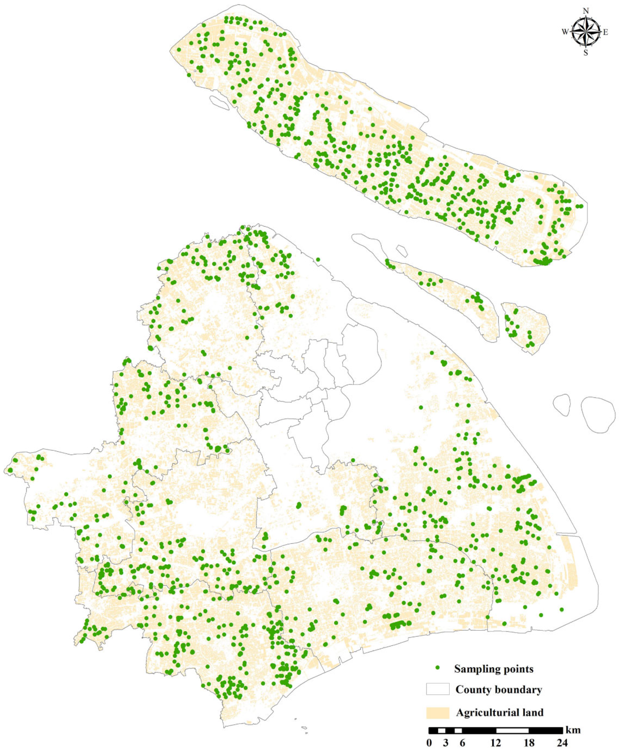
Referring to the land use map, 1848 topsoil (0–20 cm) sampling points were selected preliminarily based on a 1 km × 1 km grid covering all of the agricultural land in the study area. During sampling, the samples’ location was adjusted to acquire the cultivated soil. The distribution of the sample locations is shown in Figure 1. Detailed information about sampling, chemical analysis, and quality control can be found in previous studies [15,22]. As an overview, all samples were collected from agricultural soils using the Global Positioning System (GPS) to record the location information. Five subsamples were collected around each sampling location and then thoroughly mixed to obtain a representative composite sample. Soil samples were collected by a plastic spade, stored in polyethylene bags with labels, and returned to the laboratory for air-drying at room temperature. All operations followed The Technical Specification for Soil Environmental Monitoring (HJ/T 166-2004). In the chemical analysis procedures, soil samples were grounded to 100 mesh and then acid digested with a mixture of HCl-HNO3-HClO4. The concentrations of Pb, Cr, and Cd were measured by inductively coupled plasma-mass spectrometry (ICP-MS, TMO, USA), and the detection limits were 0.3, 0.4, and 0.01 mg/kg, respectively, while the contents of As and Hg were measured through atomic fluorescence spectrometry and the detection limits were 0.002 and 0.05 mg/kg, respectively. Blind duplicates and standard reference materials (China National Standard Materials Center, GSS-3) were also measured for quality assurance and control purposes. The recovery rate of standard samples was between 90% and 110%, and the relative standard deviation of duplicate samples was between 3% and 8%.
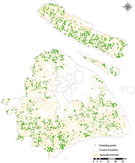
Figure 1.
Spatial distribution map of soil sampling points.
2.3. APCA-MLR Model
APCA is used to reduce data dimensionality by replacing a large set of original correlated variables with less independent variables so that major factors can be identified [30,31,32]. This is a commonly used and effective receptor model for identifying potential sources of hazardous soil contaminants [33]. The interrelationships between elements can be measured by the correlation coefficients, with higher correlation coefficients usually indicating closer relationships between TMMs that may come from the same source. During the application of APCA, a limited number of metals could offer additional useful information about sources identification [34]. The step-by-step implementation of APCA is as follows:
(i) The TMM concentration data were transformed to the dimensionless standardized form through the following equation:
where Zi,j is the standardized value of TMMs i at location j, Ci,j is the concentration of TMMs i at location j, and and are the mean and standard deviation of TMMs i throughout the entire study area, respectively.
(ii) Then, the concentration of TMMs Zi is expressed by the PCA model as:
where n is the number of sources, and ai,n and PCn are the correlation coefficient and principal components (PCs) independent of each other, respectively. Moreover, for main source identification purposes, the PCs with eigenvalues >1 after varimax rotation (Kaiser’s criterion) were extracted for further analysis [32]. The Kaiser–Meyer–Olkin and Bartlett’s sphericity tests and correlation and cluster analysis were employed to justify the reliability of PCA [5]. Cluster analysis is a typical statistical analysis technique that divides the research objects into relatively homogeneous groups. In the process of classification, cluster analysis can automatically search for object groups based on similarity for TMMs and classify different elements into the lower dimensional space. It has been demonstrated that the combination of PCA and cluster analysis leads to a more precise interpretation of the sources’ TMMs [35,36,37].
(iii) To avoid negative values of the source contribution, an artificial dimensionless standardized concentration, Zi,0, with true zero concentration, Ci,0 = 0, for each TMMs i was introduced by the following equation [18,31]:
(iv) Subsequently, the original PCs of every TMM i were estimated through the PCA method, and the absolute PCs of APCA were calculated by subtracting the factor score of the artificial sample with zero content from the original.
Finally, the MLR model was employed to calculate the contributions of source p to the concentration of TMMs i throughout the entire study area:
where Ci is the concentration of TMMs i, b0,i is the regression constant, bp,i is the regression coefficient of source p to TMMs i, n is the number of sources, and APCSp is the absolute PCs calculated from APCA analysis. The mean of the product, , represents the overall contribution of the sources [32].
2.4. APCA-GWR
MLR produces an overall model for the whole dataset that lacks the ability to deal with the important issue of the data’s spatial heterogeneity. Thus, the GWR model was proposed to replace MLR for exploring the contribution of pollution sources to TMMs from the perspective of spatial heterogeneity. The APCA-GWR model could produce a set of local regression models to describe the change in relationships between sources and pollution as follows [20,22,23]:
where i, j, and p represent TMMs i, location j, and source type p, respectively. C is the concentration of TMMs, b is the regression coefficient, APCS is the absolute factor score, and is the random error. GWR could associate a specific model to every sample through Equation (5), which can effectively address the spatial heterogeneity problem [24].
Through a distance decay function, GWR is calibrated by weighting all observations around an estimation point, assuming that the closer the distance of the observation location to the estimation point, the greater its impact on the local parameter estimates at each point [23]. Further, the weighting function is defined as follows:
where is the weight of the neighbor i to the location j, is the distance between i and j, and h is the kernel bandwidth. When the distance is greater than the kernel bandwidth, the weight rapidly approaches zero [20]. Considering the uneven distribution of samples in the study area, an adaptive kernel was used (which can adapt bandwidths in size to variations in data density), and the optimal bandwidth was determined by minimizing the corrected Akaike Information Criterion (AICc) [20,23,38].
Three indices were implemented to compare the performance of the APCA-MLR model vs. the APCA-GWR model: (1) coefficient of determination (R2), which represents the interpretation ability of independent variables (sources) to the dependent variable (TMMs); (2) AIC values, which denote the approximation of the model to reality (goodness of fit); and (3) Moran’s I of standardized residuals, which represents the model’s ability to handle a variable’s spatial autocorrelation.
The descriptive statistics (including maximum and minimum, average) and data transformation and correlation, cluster, MLR, and PCA analysis were conducted using SPSS 19.0 software (IBM Inc., Armonk, NY, USA). GWR modeling was conducted using SAM 4.0 software [39]. The spatial distribution maps were drawn through ordinary kriging in ArcMap 10.2 (Esri Inc., Redlands, CA, USA). P values at the 0.05 level were considered significant, and all P values and 95% CIs were two-sided.
3. Results and Discussion
3.1. Basic Characteristics of TMM Content in Soil
Descriptive statistics of the TMM’s contents (including minimum, maximum, mean, standard deviation, coefficient of variation, skewness, and kurtosis) in agricultural soil and their corresponding background values [40] in local regions and risk screening values in China (GB15618-2018) are shown in Table 1. In addition, the original TMM dataset, along with their locations, are shown in Supplementary Materials, Table S1. The contents of Pb, Cd, Cr, As, and Hg ranged from 12.40 to 198.00 mg/kg, 0.06 to 2.80 mg/kg, 47.00 to 152.00 mg/kg, 3.02 to 33.70 mg/kg, and 0.02 to 0.74 mg/kg, respectively, with mean values of 25.57 mg/kg, 0.19 mg/kg, 72.02 mg/kg, 6.98 mg/kg, and 0.12 mg/kg, respectively.

Table 1.
Descriptive statistics of TMM contents (mg/kg) in agricultural soils.
Compared to the local background values [40], the mean contents of Pb and As were lower than their corresponding background values, whereas the mean contents of Cd, Cr, and Hg were higher than their corresponding background values. The proportion of samples for TMM concentrations higher than their corresponding background values was in the decreasing order of Cd (46.94%) > Hg (43.81%) > Cr (41.81%) > As (37.97%) > Pb (35.42%) (Table 1), indicating that a certain amount of TMM accumulation has occurred in agricultural soils due to human activities, of which the accumulation of Cd and Hg was more serious. However, compared with the risk screening values defined by the National Environmental Quality Standards for Soils in China (GB15618-2018), the mean concentrations of these TMMs were all lower than the strictest risk screening values. The proportion of samples with TMM concentrations higher than their corresponding risk screening values was in the decreasing order of Cd (3.03%) > Hg (0.38%) > As (0.11%) > Pb (0.05%) > Cr (0.00%) (Table 1), indicating that the soil was relatively safe for agricultural production and human health.
The coefficient of variation (CV) for each element was in the increasing order of Cr (12.36%) < As (28.17%) < Pb (28.85%) < Cd (55.19%) < Hg (63.17%). The CV indicates the mean dispersion of the content, CV < 15%, between 15% and 35%, and >35%, was defined as low, moderate, and high variation [41]. Accordingly, Cd and Hg showed high variation, Pb and As showed moderate variation, and Cr showed low variation. Cd and Hg demonstrated a wider extent of variability in relation to the mean, and the high CV and strongly positive skewness of Cd and Hg indicated that they were strongly affected by human activities [19,42], whereas the low CV value of Cr indicated that it was mainly controlled by natural sources, such as soil parent material [22]. Further, Pb and As demonstrated moderate variation, which indicated the concentration distributions were relatively uneven and from composite sources [41]. According to the skewness and kurtosis values and the results of the Kolmogorov-Smirnov (K-S) normality test, the TMMs were not normally distributed. In addition, as the distributions of all elements showed a positive skewness, the logarithmic transformation was applied preceding the analysis [5].
3.2. Source Analysis through APCA
The statistical results of Kaiser–Meyer–Olkin (KMO = 0.597) and Bartlett’s sphericity tests (p < 0.01) indicated that APCA was an effective tool for the source analysis of TMM pollution in this study area [15]. In total, three PCs with eigenvalues greater than 1.0 were extracted from APCA, and they could explain 76.25% of the total TMM variation. The remaining variation (23.75%) may be due to sampling errors, chemical analysis errors, and other unidentified sources [41]. Table 2 shows the factor loading matrices (loadings greater than 0.5 are in bold) generated by APCA with the dataset of soil TMMs. PC1 was highly associated with As and Cr; PC2 was highly correlated with Pb and Hg, and PC3 was highly related to Cd. The accuracy and reliability of the APCA results can be further justified by correlation and cluster analyses: the correlation analysis showed that As and Cr (r = 0.699, p < 0.01) and Hg and Pb (r = 0.590, p < 0.01) were strongly correlated to each other, and Pb was moderately correlated to Cr (r = 0.477, p < 0.01) and As (r = 0.443, p < 0.01), whereas Cd was not related to other TMMs. Additionally, the results of cluster analysis (Figure S1) revealed that As and Cr can be classified as one group, Hg and Pb could be defined as another group, and Cd was considered individually. The specific description and discussion of each PC were as follows.
Table 2.
Results of principal component analysis.
PC1 contributed to 27.83% of the total variation in TMMs in agricultural soils. It was loaded heavily with As (0.817) and Cr (0.707) and moderately with Pb (0.454) (Table 2). According to the descriptive statistics of TMMs (Table 1), although about one-third of the samples showed As and Pb contents higher than the background values (the reason will be discussed in Section 3.4), the mean contents of As and Pb were less than their local background values [34], which indicated that anthropogenic sources had little overall effect on the accumulation of these two TMMs [19,32]. Although the mean content of Cr was higher than its local background value (the over-standard rate is 41.81%, and the reason for this will be discussed in Section 3.4), the concentrations in all areas were still under control (i.e., for Cr, the percentage of sample values higher than the risk screening values is 0%, Table 1). Moreover, Cr showed the least spatial heterogeneity, which was confirmed by the lowest CV value (CV = 12.36%), implying that Cr had few outliers caused by an anthropogenic point source (such as industrial emission) and was mainly controlled by soil characteristics [43]. The spatial distribution of PC1 can be seen in Figure S2; high PC1 values were concentrated in the eastern and northern alluvial parent material areas [44], which indicated that the geochemical characteristics of the soil were the highest contributors to Cr and As accumulation [45]. In addition, previous studies also reported that Cr and As could be mainly attributed to natural sources such as lithogenic components and soil parent material [27,46,47]. In summary, PC1 encompassed influences from natural sources such as soil parent material (especially alluvial materials) and the lithogenic process.
PC2 explained 27.80% of the total variance and was weighed heavily with Hg (0.876) and Pb (0.647) (Table 2). Based on the descriptive statistics of Table 1, Hg showed the highest CV value (63.17%), and the mean content of Hg was higher than its corresponding background value, with an excess proportion of 43.81%, which indicated that anthropogenic sources have important effects on the accumulation of this element. Previous studies have indicated that about 40% of the external Hg input to agricultural soils was from coal combustion in China, accounting for more than 70% of the total atmospheric Hg input [19,48], and the high volatilization of Hg makes it easier to enter the flue gas during coal combustion, which eventually causes Hg accumulation in soil by atmospheric deposition [49,50,51]. On the other hand, although the mean Pb content is relatively low, about one-third of the samples with Pb content exceeded the background value (Table 1). Moreover, Pb showed moderate variation (CV = 28.85%), indicating that anthropogenic point source pollution has a certain impact on its accumulation. Pb in agricultural soils was commonly caused by automobile exhaust emissions that account for roughly two-thirds of global Pb pollution [47]. Over the past several decades, due to the combustion of gasoline with tetraethyl Pb as an antiknock agent (it was banned in 2000), vehicle emissions bring large, exogenous Pb pollution to soils [15,43,52]. Additionally, coal combustion could also be an important contributor of Pb through atmospheric deposition [47]. The high PC2 values (Figure S2) were distributed in central urban and surrounding suburban areas with dense industry and transportation activities [27], which further indicated that PC2 can be considered the source of atmospheric deposition pollution from coal combustion and transportation activities.
PC3 accounted for 20.62% of the total variation and was dominated by Cd (0.959) (Table 2). The mean content of Cd was higher than its background value, with an over-standard rate of 46.94%. In addition, 3.03% of the samples revealed higher contents than the national risk screening value, indicating the severe pollution of Cd due to anthropogenic sources (Table 1). Generally, Cd, as an inherent component of phosphate rock, is transferred to phosphate fertilizers, and the mean Cd concentration in phosphate rock and fertilizer is 0.98 and 0.6 mg/kg, respectively [19], which is much higher than the background values in local soils. Thus, agricultural activities, such as the application of phosphate fertilizer, provide considerable amounts of Cd to agricultural soil. Previous studies also concluded that Cd could be considered a marker element of agricultural activities that include the overuse of pesticides and chemical fertilizers [47,53,54]. Further, the high values of PC3 were distributed in the northern mainland and Chongming Island (Figure S2), where the largest agricultural planting base in Shanghai is located [44]. Thus, PC3 could be defined as the influencer of agricultural activities, especially the overuse of phosphate fertilizer.
3.3. APCA-MLR vs. APCA-GWR
The overall contributions of each PC to the TMMs were similar between the APCA-MLR and APCA-GWR models (Table 3). Specifically, Pb was mainly attributed to PC1 (36.95% and 35.32% (mean) derived from MLR and GWR, respectively) and PC2 (52.72% and 51.46% (mean) derived from MLR and GWR, respectively); Cd mainly came from PC3 (83.86% and 82.15% (mean) derived from MLR and GWR, respectively); Cr was mainly attributed to PC1 (55.62% and 53.19% (mean) derived from MLR and GWR, respectively); As mainly came from PC1 (64.60% and 57.63% (mean) derived from MLR and GWR, respectively); and most of the Hg was explained by PC2 (82.92% and 73.61% (mean) derived from MLR and GWR, respectively). In addition, compared with the MLR model, PC3 in the GWR model showed a stronger interpretation of Cr and As, which indicates that the overuse of phosphate fertilizer and pesticides has certain influences on these elements (Table 3).
Table 3.
Mean contributions (%) of each principal component to TMMs derived from the APCA-MLR and APCA-GWR models.
Noticeably, the important advantage of the APCA-GWR model is that, in addition to analyzing the overall contribution of pollution sources to TMMs, it can also account for the spatial heterogeneity of contributions from different sources to various elements. Those differences could be initially seen in Table 3 as the standard deviation of the contributions. Due to the local regression models produced by APCA-GWR, this technique could not only calculate the average contribution of each source to TMM pollution but also estimate the specific contribution of each source to TMMs at every location (exhibited as the standard deviation of the contributions in Table 3), which can provide detailed references for pollution apportionment and control. The specific APCA-GWR pollution source analysis is discussed in Section 3.4.
Furthermore, it is worth noting that for each TMM, the APCA-GWR model had substantially higher R2 values (Pb: 0.76 vs. 0.64; Cd: 0.96 vs. 0.94; Cr: 0.79 vs. 0.67; As: 0.87 vs. 0.77; and Hg: 0.87 vs. 0.78) and lower AIC values (Pb: 2688.20 vs. 3369.87; Cd: -829.66 vs. 56.76; Cr: 2381.31 vs. 3202.38; As: 1591.40 vs. 2556.99; and Hg: 1537.42 vs. 2413.72) than the APCA-MLR model (Table 4). As indices for each model’s interpretation ability and goodness of fit, respectively, higher R2 and lower AIC values implied that the APCA-GWR model was more efficient and powerful than the APCA-MLR model in predicting the pollution sources of TMMs by including spatial heterogeneity [20,21,55]. In addition, Moran’s I of residuals calculated from the APCA-MLR model among all TMMs showed significant spatial autocorrelation. In contrast, after fitting the APCA-GWR model, Moran’s I of the predicted residuals of each element was no longer significant (Table 4), indicating that the APCA-GWR model was more powerful in explaining the spatial heterogeneity of the pollution sources [20,21].
Table 4.
Performance comparison between the APCA-MLR and APCA-GWR models.
3.4. Source Apportionment through APCA-GWR
The distributions of the R2 values that represented the explanatory power of the three principal sources (i.e., PC1: natural sources (especially alluvial materials), PC2: atmospheric deposition pollution from coal combustion and transportation activities, and PC3: agricultural activities, especially the overuse of phosphate fertilizer) to TMM pollution were shown in Figure 2. Unlike the overall R2 generated by APCA-MLR, the APCA-GWR produces a set of local equations and R2 values for all points, which is beneficial for the further analysis of the spatial heterogeneity of the sources to TMM pollution. In detail, the distributions of R2 for As and Cr were similar: strong explanatory power was exhibited in the eastern mainland and on northern Chongming Island, but the explanatory power was weak in the northern mainland. This distribution pattern was similar to the PC1 distribution (Figure S2), indicating that PC1 has the strongest explanation ability regarding As and Cr. Moreover, in the southeastern part of the mainland, As and Cr also revealed a high R2, which indicated that PC3 had certain impacts on their accumulation in these areas (Figure S2). For Pb, the R2 values were high in the eastern and northern mainland but low in the southwestern mainland. This spatial pattern was similar to the combined high values distribution of PC1 and PC2 (i.e., the high value of PC1 was clustered in the eastern part of the mainland and the northern part of Chongming Island, whereas the high value of PC2 was clustered in the suburbs, especially the northern suburbs areas (Figure 2 and Figure S2)), indicating that Pb had mixed sources. In addition, the R2 for Cd and Hg revealed high values throughout the study area except for some cold spots (low explanatory power) in the mainland and Chongming Island (Figure 2). The difference between the R2 of these two elements was that high R2 values of Hg were concentrated in the suburban areas, while high R2 values of Cd were clustered in the northern areas, indicating that PC2 and PC3 were the main influencing factors of Hg and Cd pollution, respectively (Figure S2). The spatial heterogeneity distributions of each pollution source’s contribution (bp,i,j × APCSp,i,j in Equation (5) to the TMMs are shown in Figure 3. In detail:
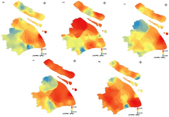
Figure 2.
Spatial distribution map of R2 from geographically weighted regression models.
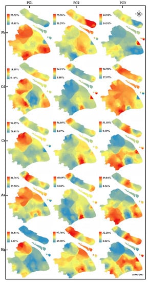
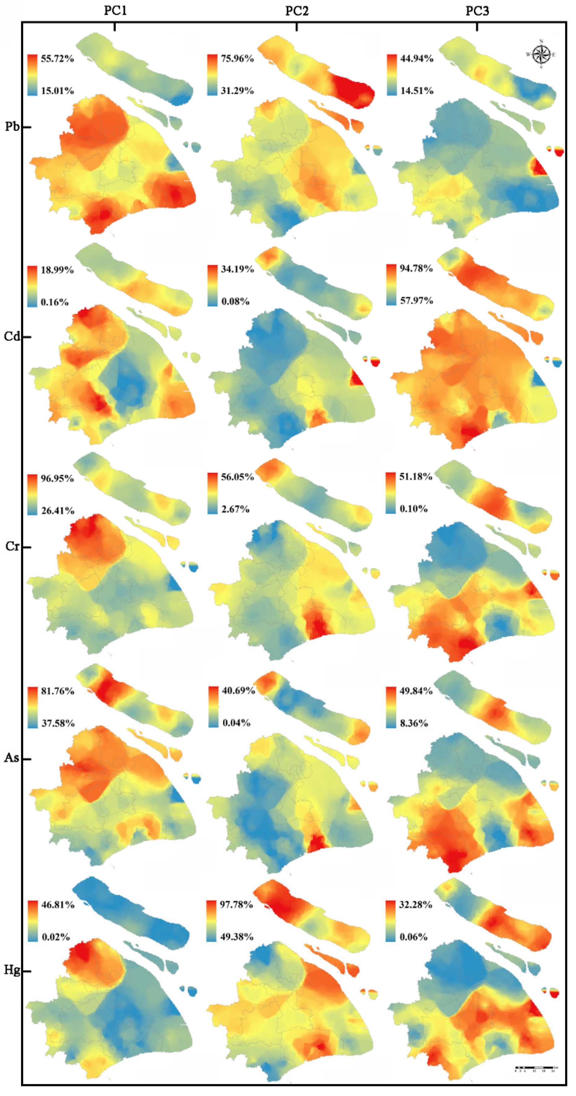
Figure 3.
Spatial distribution maps for the contributions of sources (PC1, PC2, and PC3 represent the principal components 1, 2, and 3) to each TMM from geographically weighted regression models.
As and Cr showed complex distributions of source contributions: PC1 revealed high contribution rates in the northern mainland, implying that alluvial parent material and lithogenic processes were the main sources of As and Cr in this region [46,47], whereas PC2 exhibited low contribution rates across the study area except for some hot spots on the boundary, indicating that atmospheric deposition pollution from coal combustion and transportation activities had little influence on their accumulation. In addition, PC3 exhibited great contribution rates to As and Cr in the southern mainland and the middle of Chongming Island. Chongming Island is the largest agricultural planting base in Shanghai [47] and the southern area, including the Jinshan and Fengxian districts, which are also zones where intense agricultural activities occur [41]. These results indicate that, in some specific areas, agricultural activities, especially the overuse of phosphate fertilizer and pesticides, were the main sources of As and Cr pollution, which were different from the overall APCA-MLR analysis, showing that As and Cr were mainly derived from natural sources across the study area. Those source apportionment differences further indicated that APCA-GWR provides better interpretations of the spatial heterogeneity of pollution sources than APCA-MLR. The anthropogenic sources of the two elements also explain why 37.97% and 41.81% of the samples exhibited As and Cr contents, respectively, exceeding the background value (Table 1).
PC2 exhibited high contribution rates of Pb in the eastern mainland and Chongming Island, implying that intensive traffic/transportation activities were the main reason for Pb accumulation in agricultural soil in these regions [51,52]. In addition, PC1 contributed great amounts of Pb in the northern and southern mainland, indicating that parent material and lithogenic processes are the main sources of Pb in these areas. These results also explained that although the mean Pb content was slightly lower than the background value due to the high contribution to Pb accumulation from the intensive traffic/transportation activities in the eastern areas, the over-standard Pb rate remained high (35.42%).
PC3 was the dominant contributing source of Cd. Moreover, the lowest contribution rate of PC3 was significantly higher than the highest contribution of other sources (Figure 3), implying that agricultural activities, especially the overuse of phosphate fertilizer, were responsible for Cd accumulation in agricultural land [47,54].
Additionally, PC2 was the dominant source of Hg. Moreover, the lowest contribution rate of PC2 to Hg was higher than the highest contribution of other sources (Figure 3), indicating that atmospheric deposition pollution from coal combustion and transportation activities were the main sources of Hg accumulation in the agricultural soil of the study area [51].
In summary, PC1 (natural sources, especially alluvial materials) was responsible for As and Cr accumulation in the northern mainland and Pb accumulation in the southern and northern mainland. PC2 (atmospheric deposition pollution from coal combustion and transportation activities) was the highest Hg contributor in the entire study area and the highest Pb contributor in the eastern mainland and Chongming Island. PC3 (agricultural activities, especially the overuse of phosphate fertilizer) was the main pollution source of Cd across the study area and of As and Cr in the southern mainland and the middle of Chongming Island.
4. Conclusions
Based on the detailed survey of agricultural soil TMM concentrations in this study area, it was found that Cd was the most polluting element, with proportions higher than its corresponding background and risk screening values of approximately 46.94% and 3.03%, respectively. The APCA results revealed three main sources of TMM pollution, i.e., PC1: natural sources (alluvial soil materials), PC2: atmospheric deposition pollution from coal combustion and transportation activities, and PC3: the overuse of phosphate fertilizer in agricultural activities, which could explain 27.83%, 27.80%, and 20.62% of the total variance, respectively. According to the APCA-MLR analysis, overall, Pb mainly came from PC1 (36.95%) and PC2 (52.72%), Cd was mainly attributed to PC3 (83.86%), Cr (55.62%) and As (64.60%) were mainly explained by PC1, and Hg was mainly derived from PC2 (82.92%). The APCA-GWR model generated more accurate and specific results about the source distribution than the APCA-MLR model, which was attributed to its methodological advantage that, unlike APCA-MLR, the APCA-GWR accounted for the spatial variation features of soil contamination. This superiority was quantitatively expressed in terms of higher R2 values, lower AIC values, and the non-spatial residual autocorrelation. More specifically, PC1 was responsible for As and Cr accumulation in the northern mainland and Pb accumulation in the southern and northern mainland. PC2 contributed the most to Hg in the entire study area and contributed the most to Pb in the eastern mainland and Chongming Island. PC3 was the main pollution source of Cd across the study area and of As and Cr in the southern mainland and middle of Chongming Island. In summary, the present study highlights the use of a synthetic APCA-GWR model to efficiently handle TMM source apportionment issues with in situ spatial heterogeneity, which could provide more accurate and specific pollution source information, as well as better references for pollution prevention and human health protection.
Supplementary Materials
The following supporting information can be downloaded at https://www.mdpi.com/article/10.3390/su14020783/s1. Figure S1: The results of cluster analysis; Figure S2: Spatial distribution of principal components derived from absolute principal component analysis. PC1, PC2, and PC3 represent the principal components 1, 2, and 3, respectively; Table S1: Test and locations dataset for TMMs.
Author Contributions
Conceptualization, Z.R. and X.F.; methodology, G.C. and Z.L.; validation, H.X. and X.L.; formal analysis, Z.R. and G.C.; investigation, Z.L.; resources, X.L.; data curation, Z.R. and H.X.; writing—original draft preparation, Z.R.; writing—review and editing, X.F.; visualization, Z.L.; supervision, G.C.; project administration, X.L.; funding acquisition, X.F. All authors have read and agreed to the published version of the manuscript.
Funding
This work was partially supported by the National Key Technology Research and Development Program of China (2018YFD0200500) and the National Natural Science Foundation of China (41801302 and 41671399).
Institutional Review Board Statement
Not applicable.
Informed Consent Statement
Not applicable.
Data Availability Statement
Not applicable.
Conflicts of Interest
The authors declare no conflict of interest.
References
- Zhuang, P.; Zou, B.; Li, N.Y.; Li, Z.A. Heavy metal contamination in soils and food crops around Dabaoshan mine in Guangdong, China: Implication for human health. Environ. Geochem. Health 2009, 31, 707–715. [Google Scholar] [CrossRef]
- Shao, S.; Hu, B.; Tao, Y.; You, Q.; Huang, M.; Zhou, L.; Chen, Q.; Shi, Z. Comprehensive source identification and apportionment analysis of five heavy metals in soils in Wenzhou City, China. Environ. Geochem. Health 2021, 43, 1–24. [Google Scholar] [CrossRef]
- Ihedioha, J.N.; Ukoha, P.O.; Ekere, N.R. Ecological and human health risk assessment of heavy metal contamination in soil of a municipal solid waste dump in Uyo, Nigeria. Environ. Geochem. Health 2017, 39, 497–515. [Google Scholar] [CrossRef]
- Shi, T.; Ma, J.; Wu, F.; Ju, T.; Gong, Y.; Zhang, Y.; Wu, X.; Hou, H.; Zhao, L.; Shi, H. Mass balance-based inventory of heavymetals inputs to and outputs fromagricultural soils in Zhejiang Province, China. Sci. Total Environ. 2019, 649, 1269–1280. [Google Scholar] [CrossRef] [PubMed]
- Xu, Z.; Mi, W.; Mi, N.; Fan, X.; Zhou, Y.; Tian, Y. Characteristics and sources of heavy metal pollution in desert steppe soil related to transportation and industrial activities. Environ. Sci. Pollut. Res. 2020, 27, 38835–38848. [Google Scholar] [CrossRef] [PubMed]
- MEP of China (Ministry of Environmental Protection of China). National Soil Pollution Survey Bulletin. 2014. Available online: http://www.zhb.gov.cn/gkml/hbb/qt/201404/t20140417_270670.htm (accessed on 15 March 2019).
- Hu, B.; Shao, S.; Ni, H.; Fu, Z.; Hu, L.; Zhou, Y. Current status, spatial features, health risks, and potential driving factors of soil heavy metal pollution in China at province level. Environ. Pollut. 2020, 266, 114961. [Google Scholar] [CrossRef] [PubMed]
- Chen, H.; Teng, Y.; Lu, S.; Wang, Y.; Wang, J. Contamination features and health risk of soil heavy metals in China. Sci. Total Environ. 2015, 512, 143–153. [Google Scholar] [CrossRef]
- Pourret, O. On the necessity of banning the term “heavy metal” from the scientific literature. Sustainability 2018, 10, 2879. [Google Scholar] [CrossRef] [Green Version]
- Yu, S.; Zhu, Y.; Li, X. Trace metal contamination in urban soils of China. Sci. Total Environ. 2012, 421–422, 17–30. [Google Scholar]
- Al-Hwaiti, M.; Al-Khashman, O. Health risk assessment of heavy metals contamination in tomato and green pepper plants grown in soils amended with phosphogypsum waste materials. Environ. Geochem. Health 2015, 37, 287–304. [Google Scholar] [CrossRef] [PubMed]
- Jia, X.L.; Fu, T.T.; Hu, B.F.; Shi, Z.; Zhou, L.Q.; Zhu, Y.W. Identification of the potential risk areas for soil heavy metal pollution based on the source-sink theory. J. Hazard. Mater. 2020, 393, 122424. [Google Scholar] [CrossRef]
- Feng, J.; Zhao, J.; Bian, X.; Zhang, W. Spatial distribution and controlling factors of heavy metals contents in paddy soil and crop grains of rice–wheat cropping system along highway in East China. Environ. Geochem. Health 2012, 34, 605–614. [Google Scholar] [CrossRef]
- Hu, B.; Jia, X.; Hu, J.; Xu, D.; Xia, F.; Li, Y. Assessment of heavy metal pollution and health risks in the soil-plant-human system in the Yangtze river delta, China. Int. J. Environ. Res. Public Health 2017, 14, 1042. [Google Scholar] [CrossRef] [PubMed] [Green Version]
- Fei, X.; Xiao, R.; Christakos, G.; Langousis, A.; Ren, Z.; Tian, Y.; Lv, X. Comprehensive assessment and source apportionment of heavy metals in Shanghai agricultural soils with different fertility levels. Ecol. Indic. 2019, 106, 105508. [Google Scholar] [CrossRef]
- Qu, M.; Wang, Y.; Huang, B.; Zhao, Y. Source apportionment of soil heavy metals using robust absolute principal component scores-robust geographically weighted regression (RAPCS-RGWR) receptor model. Sci. Total Environ. 2018, 626, 203–210. [Google Scholar] [CrossRef]
- Zhang, H.; Yin, S.; Chen, Y.; Shao, S.; Wu, J.; Fan, M. Machine learning-based source identification and spatial prediction of heavy metals in soil in a rapid urbanization area, eastern China. J. Clean. Prod. 2020, 273, 122858. [Google Scholar] [CrossRef]
- Jin, G.; Fang, W.; Shafi, M.; Wu, D.; Li, Y.; Zhong, B.; Liu, D. Source apportionment of heavy metals in farmland soil with application of APCS-MLR model: A pilot study for restoration of farmland in Shaoxing City Zhejiang, China. Ecotox. Environ. Safety 2019, 184, 109495. [Google Scholar] [CrossRef]
- Lv, J. Multivariate receptor models and robust geostatistics to estimate source apportionment of heavy metals in soils. Environ. Pollut. 2019, 244, 72–83. [Google Scholar] [CrossRef] [PubMed]
- Fei, X.; Chen, W.; Zhang, S.; Liu, Q.; Zhang, Z.; Pei, Q. The spatio-temporal distribution and risk factors of thyroid cancer during rapid urbanization–A case study in China. Sci. Total Environ. 2018, 630, 1436–1445. [Google Scholar] [CrossRef]
- Wang, N.; Mengersen, K.; Tong, S.; Kimlin, M.; Zhou, M.; Liu, Y.; Hu, W. County-level variation in the long-term association between PM2. 5 and lung cancer mortality in China. Sci. Total Environ. 2020, 738, 140195. [Google Scholar] [CrossRef]
- Fei, X.; Christakos, G.; Xiao, R.; Ren, Z.; Liu, Y.; Lv, X. Improved heavy metal mapping and pollution source apportionment in Shanghai City soils using auxiliary information. Sci. Total Environ. 2019, 661, 168–177. [Google Scholar] [CrossRef]
- Tu, J.; Xia, Z.G. Examining spatially varying relationships between land use and water quality using geographically weighted regression I: Model design and evaluation. Sci. Total Environ. 2008, 407, 358–378. [Google Scholar] [CrossRef] [PubMed]
- Xiao, R.; Su, S.; Wang, J.; Zhang, Z.; Jiang, D.; Wu, J. Local spatial modeling of paddy soil landscape patterns in response to urbanization across the urban agglomeration around Hangzhou Bay, China. Appl. Geogr. 2013, 39, 158–171. [Google Scholar] [CrossRef]
- Zhang, Z.; Tu, Y.J.; Li, X. Quantifying the Spatiotemporal patterns of urbanization along urban-rural gradient with a roadscape transect approach: A case study in Shanghai, China. Sustainability 2016, 8, 862. [Google Scholar] [CrossRef] [Green Version]
- Huang, Y.; Li, T.; Wu, C.; He, Z.; Japenga, J.; Deng, M.; Yang, X. An integrated approach to assess heavy metal source apportionment in peri-urban agricultural soils. J. Hazard. Mater. 2015, 299, 540–549. [Google Scholar] [CrossRef] [PubMed]
- Gao, J.; Wang, L. Ecological and human health risk assessments in the context of soil heavy metal pollution in a typical industrial area of Shanghai, China. Environ. Sci. Pollut. Res. 2018, 25, 27090–27105. [Google Scholar] [CrossRef]
- Naccarato, A.; Tassone, A.; Cavaliere, F.; Elliani, R.; Pirrone, N.; Sprovieri, F.; Tagarelli, A.; Giglio, A. Agrochemical treatments as a source of heavy metals and rare earth elements in agricultural soils and bioaccumulation in ground beetles. Sci. Total Environ. 2020, 749, 141438. [Google Scholar] [CrossRef]
- Xu, Y.; Shi, H.; Fei, Y.; Wang, C.; Mo, L.; Shu, M. Identification of Soil Heavy Metal Sources in a Large-Scale Area Affected by Industry. Sustainability 2021, 13, 511. [Google Scholar] [CrossRef]
- Ha, H.; Olson, J.R.; Bian, L.; Rogerson, P.A. Analysis of heavy metal sources in soil using kriging interpolation on principal components. Environ. Sci. Technol. 2014, 48, 4999–5007. [Google Scholar] [CrossRef]
- Chen, D.; Xie, Z.; Zhang, Y.; Luo, X.; Guo, Q.; Yang, J.; Liang, Y. Source apportionment of soil heavy metals in Guangzhou based on the PCA/APCS model and geostatistics. Ecol. Environ. Sci. 2016, 25, 1014–1022. [Google Scholar]
- Yang, Y.; Yang, X.; He, M.; Christakos, G. Beyond mere pollution source identification: Determination of land covers emitting soil heavy metals by combining PCA/APCS, GeoDetector and GIS analysis. Catena 2020, 185, 104297. [Google Scholar] [CrossRef]
- Huang, Y.; Deng, M.; Wu, S.; Japenga, J.; Li, T.; Yang, X.; He, Z. A modified receptor model for source apportionment of heavy metal pollution in soil. J. Hazard. Mater. 2018, 354, 161–169. [Google Scholar] [CrossRef]
- Guo, X.; Sun, Q.; Zhao, Y.; Cai, H. Identification and characterisation of heavy metals in farmland soil of Hunchun basin. Environ. Earth Sci. 2019, 78, 1–11. [Google Scholar] [CrossRef]
- Lee, H.G.; Kim, H.K.; Noh, H.J.; Byun, Y.J.; Chung, H.M.; Kim, J.I. Source identification and assessment of heavy metal contamination in urban soils based on cluster analysis and multiple pollution indices. J. Soils Sediments 2021, 21, 1947–1961. [Google Scholar] [CrossRef]
- Jahromi, M.A.; Jamshidi-Zanjani, A.; Darban, A.K. Heavy metal pollution and human health risk assessment for exposure to surface soil of mining area: A comprehensive study. Environ. Earth Sci. 2020, 79, 1–18. [Google Scholar]
- Keshavarzi, A.; Kumar, V.; Ertunç, G.; Brevik, E.C. Ecological risk assessment and source apportionment of heavy metals contamination: An appraisal based on the Tellus soil survey. Environ. Geochem. Health 2021, 43, 2121–2142. [Google Scholar] [CrossRef] [PubMed]
- Fotheringham, A.S.; Charlton, M.E.; Brunsdon, C. Spatial variations in school performance: A local analysis using geographically weighted regression. Geogr. Environ. Model. 2001, 5, 43–66. [Google Scholar] [CrossRef]
- Rangel, T.F.; Diniz-Filho, J.A.F.; Bini, L.M. SAM: A comprehensive application for spatial analysis in macroecology. Ecography 2010, 33, 46–50. [Google Scholar] [CrossRef]
- CNEMC. The Background Values of Chinese Soil. Environmental Science Press of China, Beijing; China National Environmental Monitoring Centre: Beijing, China, 1990. [Google Scholar]
- Li, R.; Yuan, Y.; Li, C.; Sun, W.; Yang, M.; Wang, X. Environmental health and ecological risk assessment of soil heavy metal pollution in the coastal cities of Estuarine Bay—A case study of Hangzhou Bay, China. Toxics 2020, 8, 75. [Google Scholar] [CrossRef]
- Liu, J.; Liu, Y.J.; Liu, Y.; Liu, Z.; Zhang, A.N. Quantitative contributions of the major sources of heavy metals in soils to ecosystem and human health risks: A case study of Yulin, China. Ecotox. Environ. Saf. 2018, 164, 261–269. [Google Scholar] [CrossRef]
- Cui, Z.; Wang, Y.; Zhao, N.; Yu, R.; Xu, G.; Yu, Y. Spatial distribution and risk assessment of heavy metals in Paddy soils of Yongshuyu irrigation area from Songhua River Basin, Northeast China. Chin. Geogr. Sci. 2018, 28, 797–809. [Google Scholar] [CrossRef] [Green Version]
- Sun, T.; Huang, J.; Wu, Y.; Yuan, Y.; Xie, Y.; Fan, Z.; Zheng, Z. Risk Assessment and Source Apportionment of Soil Heavy Metals under Different Land Use in a Typical Estuary Alluvial Island. Int. J. Environ. Res. Public Health 2020, 17, 4841. [Google Scholar] [CrossRef]
- Yang, S.; Taylor, D.; Yang, D.; He, M.; Liu, X.; Xu, J. A synthesis framework using machine learning and spatial bivariate analysis to identify drivers and hotspots of heavy metal pollution of agricultural soils. Environ. Pollut. 2021, 287, 117611. [Google Scholar] [CrossRef]
- Lv, J.; Wang, Y. Multi-scale analysis of heavy metals sources in soils of Jiangsu Coast, Eastern China. Chemosphere 2018, 212, 964–973. [Google Scholar] [CrossRef]
- Sun, L.; Guo, D.; Liu, K.; Meng, H.; Zheng, Y.; Yuan, F.; Zhu, G. Levels, sources, and spatial distribution of heavymetals in soils froma typical coal industrial city of Tangshan, China. Catena 2019, 175, 101–109. [Google Scholar] [CrossRef]
- Peng, H.; Chen, Y.; Weng, L.; Ma, J.; Ma, Y.; Li, Y.; Islam, M.S. Comparisons of heavy metal input inventory in agricultural soils in North and South China: A review. Sci. Total Environ. 2019, 660, 776–786. [Google Scholar] [CrossRef] [PubMed]
- Nanos, N.; Grigoratos, T.; Rodríguez Martín, J.A.; Samara, C. Scale-dependent correlations between soil heavy metals and As around four coal-fired power plants of northern Greece. Stoch. Environ. Res. Risk Assess. 2015, 29, 1531–1543. [Google Scholar] [CrossRef]
- Islam, M.S.; Ahmed, M.K.; Habibullah-Al-Mamun, M. Apportionment of heavy metals in soil and vegetables and associated health risks assessment. Stoch. Environ. Res. Risk Assess. 2016, 30, 365–377. [Google Scholar] [CrossRef]
- Hu, W.; Wang, H.; Dong, L.; Huang, B.; Borggaard, O.K.; Hansen, H.C.B.; He, Y.; Holm, P.E. Source identification of heavy metals in peri-urban agricultural soils of southeast China: An integrated approach. Environ. Pollut. 2018, 237, 650–661. [Google Scholar] [CrossRef] [PubMed]
- Guo, W.; Zhang, H.; Cui, S.; Xu, Q.; Tang, Z.; Gao, F. Assessment of the distribution and risks of organochlorine pesticides in core sediments from areas of different human activity on Lake Baiyangdian, China. Stoch. Environ. Res. Risk Assess. 2014, 28, 1035–1044. [Google Scholar] [CrossRef]
- Shao, D.; Zhan, Y.; Zhou, W.; Zhu, L. Current status and temporal trend of heavy metals in farmland soil of the Yangtze River Delta Region: Field survey and metaanalysis. Environ. Pollut. 2016, 219, 329–336. [Google Scholar] [CrossRef] [PubMed]
- Jiang, X.; Xiong, Z.; Liu, H.; Liu, G.; Liu, W. Distribution, source identification, and ecological risk assessment of heavy metals in wetland soils of a river–reservoir system. Environ. Sci. Pollut. Res 2017, 24, 436–444. [Google Scholar] [CrossRef] [PubMed]
- Mayfield, H.; Lowry, J.; Watson, C.; Kama, M.; Nilles, E.; Lau, C. Use of geographically weighted logistic regression to quantify spatial variation in the environmental and sociodemographic drivers of leptospirosis in Fiji: A modelling study. Lancet Planet Health 2018, 2, e223–e232. [Google Scholar] [CrossRef]

Publisher’s Note: MDPI stays neutral with regard to jurisdictional claims in published maps and institutional affiliations. |
© 2022 by the authors. Licensee MDPI, Basel, Switzerland. This article is an open access article distributed under the terms and conditions of the Creative Commons Attribution (CC BY) license (https://creativecommons.org/licenses/by/4.0/).