Abstract
This study investigates the relationship between climate variables such as rainfall amount, temperature, and carbon dioxide (CO2) emission and the triple dimension of food security (availability, accessibility, and utilization) in a panel of 25 sub-Saharan African countries from 1985 to 2018. After testing for cross-sectional dependence, unit root and cointegration, the study estimated the pool mean group (PMG) panel autoregressive distributed lag (ARDL). The empirical outcome revealed that rainfall had a significantly positive effect on food availability, accessibility, and utilization in the long run. In contrast, temperature was harmful to food availability and accessibility and had no impact on food utilization. Lastly, CO2 emission positively impacted food availability and accessibility but did not affect food utilization. The study took a step further by integrating some additional variables and performed the panel fully modified ordinary least squares (FMOLS) and dynamic ordinary least squares (DOLS) regression to ensure the robustness of the preceding PMG results. The control variables yielded meaningful results in most cases, so did the FMOLS and DOLS regression. The Granger causality test was conducted to determine the causal link, if any, among the variables. There was evidence of a short-run causal relationship between food availability and CO2 emission. Food accessibility exhibited a causal association with temperature, whereas food utilization was strongly connected with temperature. CO2 emission was linked to rainfall. Lastly, a bidirectional causal link was found between rainfall and temperature. Recommendations to the national, sub-regional, and regional policymakers are addressed and discussed.
1. Introduction
Food security is one of the most trending topics and a growing concern of the century. In 2020, approximately 690 million people (8.9% of the global population) were projected to be in a state of hunger [1]. The recent COVID-19 pandemic has exacerbated global hunger [1]. The number of undernourished people worldwide is likely to have risen between 83 and 132 million and could reach 840 million (9.8%) by 2030 [2]. More than 20% of the SSA population lives in food insecurity on average [3].
In 2015, the United Nations rated “ending hunger, achieving food security, enhancing nutrition, and promoting sustainable agriculture” the second among 17 Sustainable Development Goals for 2030, emphasizing food security [4]. However, while food systems are being transformed to make healthier diets more available globally, hunger, on the other hand, remains a challenge. The global undernourished population is still increasing [5], making the UN’s 2030 goal more perplexing to attain [6].
Food insecurity is more exacerbated by climate change and its variability. It is expected that mean and annual peak temperatures will continue to rise, despite overall higher average rainfall. Several temperature observations collected in SSA show statistically substantial evidence of global warming between 0.5 and 0.8 degrees Celsius (°C) between 1970 and 2010 over Africa utilizing remotely sensed data originally described [7]. SSA is one of the most vulnerable regions to rising temperatures and unpredictable wet weather [8]. For example, rainfall in West Africa’s semi-arid and sub-humid zones was 15–40% lower on average over the previous 30 years (1968–1997) than between 1931 and 1960 [9]. There was a 2.8-fold decrease in water availability throughout Africa and a 40–60% decrease in the average river discharge in West Africa [10]. By 2025, up to 370 million people in Africa will be under water stress [11]. The Central and Eastern African regions are the most vulnerable [12]. Studies in Chad revealed a strong diminishing trend of rainfall for three decades, especially during the dry season, causing drought conditions for many years. As for temperature, each of the three decades has witnessed a rise of 0.15 °C from 1950 to 2014 [13]. Both rainfall and temperature fluctuations were unequally distributed across the country [14].
Agriculture is the economic backbone of most SSA economies, accounting for up to 14% of gross domestic product (GDP) [15]. In 2019, it employed 52.9% of the workforce in the sub-region [16]. However, agriculture is still traditional and very sensitive to climate change. Rainfed agriculture is prevalent in most countries. Increasing temperatures and shifts in rainfall patterns have affected agricultural production with significant drops in crop and livestock production, thus impacting food distribution [17].
In the light of the above food security concern, this study investigates the long-run effects of climate change on food security measured by three of its indicators over the period 1985–2018 from 25 sub-Sahara African countries. Research in 2019 assessed the impact of rainfall variability on food security [18]. Few other studies evaluated climate change’s effect on crop yield [19,20,21]. Furthermore, the impact of climate change on food accessibility was thoroughly discussed [2,22,23,24,25]. A few other studies emphasized the relationship between crop nutritional value and climate change [26,27,28,29,30]. However, these studies mainly focused on a single climate variable and one indicator of food security. The uniqueness of this study lies in its attempt to go beyond previous empirical investigations by incorporating three food security indicators (food availability, accessibility, and utilization) into a single study. Cereal crops (i.e., maize, rice, millet sorghum, and wheat) are chosen as the study’s primary focus because they are the primary source of dietary energy in the diets of SSA people [31]. They are high in energy, carbs, protein, fiber, and macronutrients, particularly magnesium and zinc [32].
Cereal yield (CY) serves as a proxy measure of food availability. Food accessibility is measured by the agriculture gross domestic product (GDPA), while food utilization is determined by the Cereal Dietary Energy Supply (CDES). The motives for including these three variables are first because they comprehensively measure the three food security indicators. A pragmatic policy-oriented discussion, based on empirical determinants and relative effects, is likely to coincide with such studies. Second, it is difficult to reach a conclusion based solely on the impact (positive/negative) of the absolute value of food availability, which most researchers consider when gauging food security at the aggregate level. Third, climate variability and change directly affect food availability by increasing or reducing agriculture yields, impacting the total domestic food supply. Another reason is that agriculture GDP measures agriculture contribution to economic growth (agriculture value-added). Agriculture is SSA’s first job provider involving more than 50% of the population. Even though its share in the total GDP has reduced in recent years, it is a good indicator of farmers’ economic wellbeing, without which they could not afford food commodities. Finally, because of the data unavailability on the nutritional value of food in the sub-region, the study uses cereal dietary energy supply to represent food utilization. Cereal dietary energy supply measures the total calories provided by cereal consumption daily and is paramount in the SSA population food diet. On this premise, cereal dietary energy supply is used as a proxy for food utilization.
The rest of the paper is structured as follows: Section 2 provides empirical literature of the previous studies on related topics. Section 3 describes the data, materials, and methods, while Section 4 presents the empirical results. Section 5 is devoted to the discussion of the results. Lastly, Section 6 presents the conclusion and policy implication.
2. Literature Review
2.1. Climate Change and Food Availability
The supply side of food security is addressed as food availability. Domestic food production, commercial food imports and exports, food aid, and domestic inventories all contribute to the total amount of national food availability. Food availability is the most broadly used, studied, and researched aspect of food security. Climate uncertainty impacts agricultural-related activities, particularly production, impacting food availability (crops and livestock). Climate change has a few favorable effects, such as a prolonged agricultural season in northern latitudes. However, most of the previous findings on cereal crops across geographic locations for each predicted climatic scenario are consistent with the negative effect of climate change on crop production [33,34].
Climate change factors, including CO2 emissions, average temperature, and average precipitation, positively influence wheat productivity in Pakistan both in the short-run and long-run [35]. Likewise, an increase in annual temperature decreases both date and cereals output, while cereals production is positively affected by the yearly rainfall in Tunisia [36]. Rainfall variability and change worsen food insecurity by lowering per capita food supply, increasing the undernourished population [18]. Drought is one of the causes of malnutrition, hunger, and undernutrition. It has lowered the global food supply by producing a global grain deficit [37,38]. Lack of water inhibits plant productivity and growth, decreasing carbon absorption and higher vulnerability to pests and diseases [39].
A systematic analysis of crop production in Africa and South Asia highlighted a possible decline in crop yields by 8% by 2050. More importantly, crop yields were anticipated to fall by 17% (wheat), 5% (maize), 15% (sorghum), and 10% (millet) across Africa as against 16% (maize) and 11% (sorghum) across South Asia as a result of climate change [19]. Similarly, an increment of 20% in intraseasonal precipitation variability reduces maize, sorghum, and rice yields in Tanzania by 4.2%, 7.2%, and 7.6%, respectively [20].
Furthermore, temperature changes can affect the yield of crops. For instance, higher temperatures may accelerate plant carboxylation and boost photosynthesis, respiration, and transpiration. Higher temperatures can partly stimulate blooming, while low temperatures can reduce energy use and increase sugar storage. The emergence of new diseases in grain crops due to climate change, such as wheat blasts, poses a challenge to farmers and jeopardizes their food supply [40].
A study conducted in the Gambia found a steady negative relationship between minimum temperature, maximum temperature, and detrended yields [41]. A slight temperature rise in temperate regions (1–3 °C mean temperature, not more than 3 °C) is beneficial for crop yields. Increased evaporative heat and agricultural water stress will occur as temperatures rise in tropical areas. The rising global temperature would have disastrous effects on tropical agriculture, particularly in developing countries [42]. Similarly, Iizumi et al. (2021) [43] analyzed the consequences of rising temperatures on Sudan’s domestic wheat output and consumption by 2050 under two distinct warming scenarios (1.5 °C and 4.2 °C) and five different socioeconomic scenarios (SSPs). Even with similar future investment, technology development, and crop management assumptions, it is assumed that climate change would lead to a wheat supply deficit in Sudan by 2050.
2.2. Climate Change and Food Accessibility
Food accessibility refers to food prices, availability, and preferences that enable people to turn their hunger into need [44] effectively. Climate change impacts food production and farmers’ income, accessibility, supply, and security [22].
Many countries’ local food supplies mainly depend on global food markets, but climatic factors change agricultural products at national and regional levels [45]. Crop failures resulting from climate change negatively impact developing countries, lacking preparedness skills and ability [46].
Studies have found rainfall variability to affect smallholder crop income during the cropping season substantially negatively [22]. Similarly, a study conducted in Nepal found an increase in temperature and rainfall to negatively impact the net wheat revenues [21]. Declining agricultural productivity will intensify poverty and restrict access to food by the poor in rural and urban areas [23]. Climate variability has a significant and negative impact on economic growth in developing countries [47]. Developing countries’ financial resources are vulnerable to climatic fluctuations because a disproportionate share of their GDP is spent in climatically sensitive sectors. A reduction in agricultural production, exports, and investments in research and development can reduce output and the economy’s ability to grow. Similarly, climate shocks will decrease the amount of money available to governments by impacting economic development (low tax revenues, for example) [47].
Extreme weather occurrences can also affect the supply of food products, resulting in price increases and a reduction in the livelihood of the poor, especially in low-income countries. Consequently, allocating a high proportion of revenues toward food supplies would negatively impact people’s purchasing power [44,48,49]. This scenario would lead to worldwide hunger and food insecurity, worsened by high food costs, climate extremes, fluctuation, and limited access to food [2]. Climatic instability, for instance, increases childhood hunger in sub-Saharan Africa by rising food prices [50].
Household food budgets are tested when climate change impacts income sources [24]. An increase in food prices will influence the accessibility to and use of food, putting around 38 million people in Asia and the Pacific at risk of starvation [25]. Farmers who cultivate, process, and eat food directly from their farmland, such as subsistence and smallholder farmers, are expected to be the most exposed to climate change repercussions [51,52]. Those smallholders depend on farm productions for most of their income [53].
It has also been argued that reaching a high GDP comes with a high level of CO2 emission [54,55]. Likewise, studies examined the relationship between CO2 emission and GDP and showed a long-run causal relationship between the two [56,57,58].
2.3. Climate Change and Food Utilization
Food utilization refers to a person’s or a family’s ability to consume and profit from food [59]. In changing climatic conditions, food utilization is the least studied but most dramatically influenced component of food security [59]. Because actual food distribution across diverse populations, localities, and households is primarily understudied, focusing on food availability rather than food intakes has several drawbacks [60].
The majority of micronutrients consumed by poor households are obtained from plant consumption. Climate change could directly impact micronutrient consumption in three ways: affecting crop yields of essential micronutrient sources, changing the nutritional composition of a specific crop, or impacting crop selection decisions [61]. Additionally, price increases due to climate change result in a significant decrease in the consumption of all food groups, lowering nutrient intake. The poorest people in the country, who already spend most of their income on food, will continue to use negative coping strategies like eating less, relying on lower-quality food, and decreasing expenditure on non-food items such as health care and education [23]. To adapt to these conditions, farmers minimize the daily food consumption of all household members equally or prioritize the household’s breadwinners in times of food scarcity [62]. For instance, farmers in Nyando district, Western Kenya, were compelled to cut their food intake due to the impact of hazardous climatic events, which limited the content, variety, and frequency of meals consumed daily [52]. Smallholder farmers in Madagascar responded to food scarcity by eating smaller meals per day, modifying their food ingredients, and substituting wild plants [53].
Climate variability affects grain quality [63,64]. Zinc and iron insufficiency is frequent in low-income areas, such as sub-Saharan Africa and South and Southeast Asia, depending on grain diets, creating a severe global human health concern [27]. A study on climate change and its impact on child malnutrition among subsistence farmers in low-income nations discovered a strong relationship between weather and child stunting [28]. Climate change hinders access to food nutritional values and safe drinking water, increasing the risk of vector and waterborne diseases [28,61]. It also restricts access to proper sanitation facilities, facilitating diarrhea conditions, a leading cause of death (particularly vulnerable to climate change). As a result, it can directly cause infant morbidity and low food utilization by restricting nutrient absorption [61]. Climate change will increase diarrhea by approximately 10% in some geographical areas by 2030 due to water shortage, while higher temperatures accelerate pathogen growth [65].
Climate change could also increase new pest and disease trends and enable vector-borne diseases to become more frequent in places prone to floods, affecting human health [66]. Moreover, increased temperatures can affect pathogen and toxin exposures. This is the case regarding Salmonella, Campylobacter, and Vibrio parahaemolyticus in raw oysters, and mycotoxigenic fungi, all of which canthrive better in warmer temperatures [30].
Higher CO2 concentrations can speed up the growth of some crops, causing a decrease in nutrient quality of staple plants such as potatoes, barley, rice, and wheat [67,68,69]. Many staple crops had higher carbohydrate concentrations and lower plant-based protein and mineral content in laboratory studies of the impact of CO2 on human nutrition [29]. Increased carbon dioxide levels in the environment can also reduce dietary iron, zinc, protein, and other macro- and micronutrients in some crops [30]. For instance, Weyant, C. et al., (2018) [70] estimated that an additional 125.8 million disability-adjusted lives could be attributed to the impacts of rising atmospheric CO2 on zinc and iron levels (95% reliable interval 113.6138.9), globally between 2015 and 2050, owing to an increase in infectious diseases, diarrhea, and anemia. Notwithstanding CO2 is plant food, however, changes in plant chemistry produced by CO2 would have global implications for all living creatures that consume plants, including humans.
3. Materials and Methods
3.1. Data and Variables
The current empirical research included 25 SSA countries’ secondary panel data from 1985 to 2018. A summary of the variables used in the study is provided in Table 1.

Table 1.
Variables Description and Data Source.
3.2. Cross-Sectional Dependency Test
This research used the cross-sectional dependency method to determine which test best detects unit root problems. Cross-sectional dependence distorts the orthodox panel unit root and cointegration tests, making them ineffective. If cross-dependence is established, augmented tests such as the cross-sectionally augmented Im–Pesaran–Shin (CIPS) test and the Westerlund error-correction dependent cointegration test must be used [71,72]. Thus, the Breusch–Pagan test will be used to check any cross-sectional dependency [73]. This test is focused on the Lagrange multiplier (LM) statistic used to evaluate the null hypothesis of zero cross equation error correlations and the CIPS test. The test is recommended for small samples with a small T dimension run for that purpose. The mathematical equation of the LM cross-sectional dependence test is given below, adopted from [74,75].
where is the sample estimates of the pairwise correlation of residuals,
However, Breusch and Pagan (1980) [73] elucidate that the LM test is only valid for large N and small T. Considering this shortcoming, Pesaran (2004) [76] addresses this weakness by introducing the cross-sectional dependence test among errors which is helpful for a variety of panel data models. The unit root dynamic heterogeneous panels and stationary with big N and small T are included in this test. The results are robust to multiple or single structural breaks in single regression and slope coefficient error variance. As stated in the LM test, Pesaran (2004) [76] introduced the pairwise correlation coefficients dependence test instead of the squares of correlation [74,75].
3.3. Panel Unit Root and Cointegration Tests
The unit root and cointegration tests were performed after testing for cross-sectional independence and failing to reject the null hypothesis of cross-sectional independence. The central assumption of the panel cointegration approach used in this study is that all the variables have a unit basis. After examining the cross-sectional dependency, this study used Pesaran’s second-generation panel unit root test [77]. The Pesaran unit root test builds the test statistics and uses the cross-section mean to proxy the common factor, keeping in mind the t ratio of the ordinary least square estimator in the cross-sectional augmented Dickey–Fuller (CADF) regression.
However, one way is to use the mathematical calculations below to consider the expanded version of the CIPS test:
Additionally, for the ith cross-section unit, (n, T) denotes the ADF statistics across the cross-section, which is determined by the t ratio of coefficient ( in CADF regression.
The next step was to conduct the cointegration test for heterogeneous panels on panel data, assuming cross-sectional independence and non-stationarity of the variables. The Westerlund (2007) [72] cointegration test was run. The latter is a second-generation cointegration test, which uses the bootstrap method to produce the sample and a new sample to create two-panel statistics and two groups’ mean. This method determines whether the model has converging error terms for the entire panel or individual classes. This method assesses the model to see if it has converging error terms for the whole panel or specific groups:
where the term indicates the speed of adjustment. means that variables are not cointegrated and that there is no error correction term, whereas 0 denotes that error correction is present and that variables are cointegrated [75].
3.4. Pooled Mean Group (PMG) Estimator
The panel autoregressive distributed lag (ARDL) approach was employed to evaluate the long-run relationships between the variables and extract the ECM (error correction version) of the panel characteristics for the short-run dynamic. In addition, substitute cointegration methods, such as the Johansen and Juselius (1988) [78] and traditional Johansen [79] methods, were used to achieve similar results. However, the panel ARDL technique was chosen over cointegration because of its beneficial features. The standard cointegration approach examines the long-term relationship within the system of equations in the background, whereas the panel ARDL employs an individually briefed form of equation [80]. Regardless of whether the tested variables were I(0), I(1), or both I(0) and I(1), the panel ARDL approach could be applied [81]. Many lags can exist in a panel ARDL with multiple variables in the equation, which are unsuitable when using the typical cointegration test.
Furthermore, panel ARDL simultaneously generates long-term and short-term coefficients [66,82]. Equation (7) shows the popular output function of panel ARDL that should be studied for the bounds test approach [83]:
where = 1, 2, …, N and t = 1, 2, …, T, is an intercept term, is a k × 1 vector of coefficients (which are allowed to be heterogeneous and vary across countries) and is a k × 1 vector of the explanatory variable. can be divided into two regressor subsets, and . The resulting autoregressive distributed lags (ARDL (p, q)) specification can be generated by extending the model to a dynamic panel specification and including lags of the dependent variable as well as lagged independent variables:
The below ECM equation can be adjusted in:
where
and
The term in parentheses denotes the long-run link between the dependent and explanatory variables, and is the vector of long-run elasticity. When there is a long-run connection between the dependent and independent variables, the parameter (speed of adjustment term) is significantly different from zero. Under the hypothesis that the variables converge to long-run equilibrium, is projected to be significantly negative. Different ways to estimate the dynamic heterogeneous panel model can be utilized when the N and T dimensions are large. If only the intercepts differ between classes, a dynamic fixed-effects (DFE) estimator can be used. This method produces inconsistency in estimations when the homogeneity of slope coefficients is insufficient. The intercepts (long and short-run) slopes and error variances are varied across groups. However, the model can be estimated independently for each group, and a simple average of the coefficients is assessed, providing Pesaran and Smith’s mean group estimator.
PMG estimate introduced by Pesaran and Smith (1999) [84] was employed. This method combines pooling and averaging and can be considered a middle ground between DFE and MG (mean group) estimators [85]. Intercepts, short-run coefficients, and error variances are unregulated and differ between classes in the PMG estimator, while long-run coefficients must be homogeneous (i.e., , ∀i).
The estimating model thus becomes:
3.5. Robustness Test
Panel dynamic ordinary least squares (DOLS) and fully modified ordinary least squares (FMOLS) were used to confirm the PMG model’s results against the model’s supposed endogeneity and serial correlation problems as a robustness measure. Pedroni (2004) [86] proposes FMOLS and DOLS to obtain the long-run cointegrating coefficients. When there are “unit root variables,” the influence of super reliability may not be enough to manage the regressors’ endogeneity problem effect if ordinary least square is used. The authors [87] suggested that the FMOLS estimator postulates optimal estimates for cointegrating regressions. This method modifies the least squares to account for “serial correlation” effects as well as “endogeneity” in the regressors caused by the existence of a cointegrating interaction [88]. Furthermore, FMOLS asymptotic behavior was further explored in models with the full rank I(1) regressors, models with I(1) and I(0) regressors, models with unit roots, and models with solely stationary regressors [89]. The fully updated estimator was constructed to evaluate cointegrating relationships by explicitly adjusting conventional OLS. The FMOLS corrections can assess how significant these effects are in scientific practice, which is one reason why this technique has proven to be helpful in practice. As a result, the method has become less of a “black box” for clinicians. When there are substantial variations with OLS, the source or causes of those differences are usually easy to find, which helps to empower the researcher by offering more information about essential data properties. Recent simulation experience and empirical research suggest that the FM estimator outperforms alternative approaches for estimating the cointegrating relationship [90,91,92,93]. DOLS and FMOLS estimates are preferable to OLS estimates for a variety of reasons: (1) although OLS estimates are pretty trustworthy, the t-statistic has become non-stationary, and the I(0) terms are only approximately regular [94]. (2) Although OLS is super-consistent, OLS estimates may encounter serial correlation and heteroskedasticity in the presence of “a strong finite sample bias” because the excluded dynamics are captured by the residual, rendering regular table inference invalid even asymptotically [95]. As a result, “t” statistics for OLS estimates are useless. (3) DOLS and FMOLS address endogeneity by using leads and lags in their models (DOLS). Aside from that, white heteroskedastic norm errors are employed [96,97].
The panel DOLS model will be estimated as:
where refers to the matrix of our independent variables and the interaction term. While is the vector of all the coefficients of the regressors. DOLS regression corrects endogeneity and serial correlation through differenced leads and lags, prevalent with the ordinary least square estimator. The following equation might be used to express this:
If and are I(1) and cointegrated, the authors’ [98,99] methodology can be used to estimate the long-run coefficients of OLS and DOLS as follows:
where and are the dependent variable and the vector of independent variables.
The panel FMOLS will be estimated as:
where and stand for the endogeneity of regressors and serial correlation in error correction terms, respectively. Equations (17) and (18) express the endogeneity and serial correlation correction terms, respectively:
where and are the long-run covariance matrices computed using the residuals . is the residual computed from Equation (19) and is obtained directly from Equation (21) or indirectly from Equation (22):
is assumed strictly stationary with zero mean and infinite covariance matrix ∑.
3.6. Heterogeneous and Panel Causality
A deeper understanding is gained by tracing the causal links between variables toward empirical results’ policy implications [100]. Therefore, this study has incorporated the Granger panel causality test [101]. Correlation does not mean causation. The Granger solution to whether causes is to assess how much of the current can be described by past values, and then to see if introducing lagged data can improve the explanation. If helps in the prediction of , or if the coefficients on the lagged ’s are statistically significant, is said to be Granger caused by [102].
For a case with only two variables, the model can be written as follows:
where to and to are coefficients for the lagged dependent variables, and to and to are coefficients for the lagged independent variables. For all possible pairs of () series in the group, the reported F-statistics are the Wald statistics for the joint hypothesis for each equation:
The null hypothesis is that in the first regression, does not Granger cause , and in the second regression, does not Granger cause .
The coming sections will address climate change and food availability, climate change and food accessibility, and climate change and food utilization as models 1, 2, and 3.
4. Results
The estimation process begins with the descriptive statistics of the variables included in the study (Table 2). Secondly, cross-dependency tests are run to check the existence of cross-sectional dependence between the variables. Table 3 reports Breusch–Pagan and Pesaran tests for cross-sectional dependence test statistics and p-values. Both tests reject the null hypothesis of cross-sectional independence as they are all significant at a 1% level in all three cases, meaning there is a cross-sectional dependence. The third step consists of testing the presence of unit root in the variables. For this purpose and based on the previous cross-dependency test, two second-generation unit root tests such as the Pesaran cross-section augmented Dickey–Fuller unit root test and cross-section Im–Pesaran–Shin are the best unit root tests to use. As clearly presented in Table 4, some variables are stationary at the level. In contrast, others become stationary after the first difference, a combination of I(0) and I(1), suitably fitting panel ARDL estimators’ application.
Table 2.
Summary statistics.
Table 3.
Cross-section dependency tests.
Table 4.
Unit root test.
The fourth step is Westerlund’s (2007) [72] cointegration test (Table 5). The idea is to see whether there is an error correction model (ECM) for individual panel members or the entire panel by testing for no cointegration. The null hypothesis of no cointegration and the alternative hypothesis can be evaluated using two separate tests: group mean tests (G) and panel tests (P). Westerlund’s (2007) test produces four-panel cointegration test statistics (Gt, Ga, Pt, and Pa) based on the error correction model (ECM). The p-value and the robust p-value are above 10%; therefore, the null hypothesis of no cointegration in a heterogeneous panel could not be rejected in all three cases, indicating that the variables have no cointegration in the long run.
Table 5.
Cointegration tests.
The study uses three different techniques to estimate the long-run relationship between the variables after testing for cointegration. These techniques include pool mean group (PMG), panel dynamic ordinary least square (DOLS), and panel fully modified ordinary least square (FMOLS).
4.1. Impact of Climate Change on Food Availability
Table 6 reports the PMG estimation results. The results show that rainfall amount and CO2 emission have a positive and significant effect on food availability in the long run. In contrast, temperature change depicts a negative and significant impact. Two robustness checks are implemented. First, the model includes the GDP and land under cereal production as control variables. Both have a positive and significant impact on food availability. Second, panel FMOLS and DOLS are estimated (Table 6). The results confirm the PMG estimation’s findings except for rainfall in the DOLS model, which negatively impacts food availability.
Table 6.
Model 1 PMG, DOLS, and FMOLS.
4.2. Impact of Climate Change on Food Accessibility
The result from the PMG estimation (Table 7) highlighted a significantly positive effect of rainfall on food accessibility. However, the impact of the temperature is negative instead. CO2 emission does not affect food accessibility. In addition to that, other control variables such as cereal production quantity, GDP, and inflation rate are added for the first step of the robustness check. An increase in cereal production quantity and GDP are revealed to influence food accessibility positively and substantially, while the inflation rate affects food accessibility negatively. The second step of the robustness check consists of estimating the FMOLS and DOLS (Table 7). Both estimators’ results show a significantly positive effect of rainfall and a negative impact of CO2 emission on food accessibility.
Table 7.
Model 2 PMG, DOLS, and FMOLS.
4.3. Impact of Climate Change on Food Utilization
The PMG estimation results in Table 8 show a positive and significant rainfall effect on food utilization. In contrast, temperature and CO2 emission respectively exhibit a negative and positive but non-significant effect on food utilization. Furthermore, some control variables (cereal production, GDP, and population growth) are added, and the panel FMOLS and DOLS are estimated for the robustness check. Cereal production and GDP positively influence food utilization. However, population growth has the opposite effect. The FMOLS and DOLS results depict a positive effect of rainfall, whereas temperature and CO2 emission negatively affect food utilization. However, rainfall effect is insignificant in both outputs, while temperature does not affect food utilization in DOLS output.
Table 8.
Model 3 PMG, DOLS, and FMOLS.
4.4. Pairwise Granger Causality Tests
The study also checked the causal relations among the variables by performing the Granger causality test. Table 9, Table 10 and Table 11 outputs exhibit positive and short-run causal relationships among the variables. There is evidence of unidirectional causality running from food availability to CO2 emission. Land under cereal production Granger causes food availability and CO2 emission. Food accessibility exhibits a causal association with temperature. Similarly, there is evidence of a causal association between food accessibility and inflation rate, whereas food accessibility is Granger caused by GDP. Another unidirectional causality runs from temperature to food utilization. Furthermore, a causal connection between rainfall and CO2 emission is observed. Temperature is associated with land under cereal production, whereas GDP Granger causes temperature. There is substantial evidence of a causal association between GDP and temperature, while another causality relationship runs from temperature to cereal production. The latter, in turn, Granger causes CO2 emission and inflation rate, respectively. CO2 emission has a causality association with population growth while being Granger caused by cereal production. Likewise, temperature is associated with cereal production and population growth. The final unidirectional causal relationship runs from GDP to temperature.
Table 9.
Model 1 pairwise Granger causality test.
Table 10.
Model 2 pairwise Granger causality test.
Table 11.
Model 3 pairwise Granger causality test.
Several bidirectional causal relationships are observed. The first four observed bidirectional Granger causality are between food availability and GDP, food accessibility and temperature, food accessibility and cereal production, and between food utilization and population growth. Furthermore, bidirectional associations are observed between rainfall and temperature, and GDP. Lastly, cereal production and population growth, on the one hand, and GDP and population growth, on the other hand, share bidirectional Granger causality.
Figure 1 presents a summary of the study’s main findings.
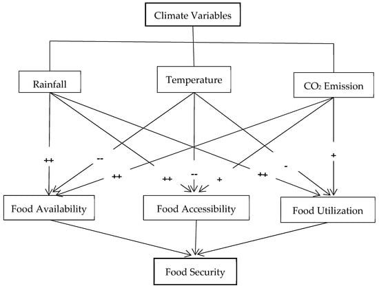
Figure 1.
Summary of the study’s main findings. ++ indicates significantly positive effect, −− indicates significantly negative effect, + and – indicate non-significant positive and negative effect.
5. Discussion
To gain new insight on the effect of climate change on food security in SSA, this study, a first of its kind, attempted to determine the direct impact of climate change (represented by rainfall, temperature, and CO2 emission) on food security as a whole through three of its indicators (food availability, accessibility, and utilization). The results acquiescently show a statistically significant and positive long-run relationship between rainfall and food availability and between CO2 emission and food availability. In contrast, temperature change has a significantly negative impact on food availability. The positive effect of rainfall on food availability is strongly substantiated by Kinda and Badolo (2019) [18]. This empirical result underlines the first-degree importance of rainfall to food availability. It plays a crucial role in improving the cereal crop yield [103] in SSA where the daily nutrients are mainly extracted from cereal consumption. Technologies such as irrigation systems with a great potential to increase crop productivity [104,105,106] are lacking in SSA countries [107]. Water from rainfall is the primary source of water used for agricultural purposes. Such high dependence on rainfall and climate predictions makes SSA uncertain whether Africa will achieve its food security goal in the nearest future. The positive impact of CO2 emission on the available food reported in the study corresponds with previous studies’ estimates [70,108,109,110,111]. An increasing amount of atmospheric CO2 is beneficial for plant growth. Higher CO2 levels are widely recognized to stimulate plant photosynthesis and development, potentially increasing cereal crop yield, which remains the world’s most important food source [108]. However, few studies found a harmful impact of CO2 emission on cereal crops production [112,113].
Temperature significantly and negatively influences crop production. These results are substantial with previous research findings [41,43,114,115]. This finding indicates that a slight increase in temperature in SSA countries where the climate is tropical and seasonally dry negatively affects crop production, and thus the quantity of available food in the sub-region. Many plant species are temperature sensitive; consequently, an increase in global temperature had adverse effects on crops production [36,116,117].
Further results indicated a positive and significant effect of rainfall on food accessibility. However, the impact of the average temperature yielded a negative effect. This outcome is not surprising as it has been established that households’ food budgets are directly affected by the impact of climate change on income sources [24]. As a result, the price of food increases, ineluctably affecting food accessibility [25]. Recent World Bank estimations show that in 2020, 58.75% of the SSA populations were living in rural areas [118], with agriculture being the primary source of income. Subsistence farmers in low-income countries usually cultivate crops adapted to their region’s long-term precipitation patterns [119,120]. However, yields can suffer when rainfall levels in a given season are significantly below long-term norms [121,122], thus affecting all the people living on agricultural activities. Food costs are rising as yields and livestock production drop, making food accessibility difficult for low-income households [123,124]. Simultaneously, families who earn their living from agricultural commodity businesses may see a decrease in their revenues [125,126,127]. Temperature change negatively impacts farmers’ net income by facilitating extreme events such as drought in rainfed areas, harming livestock, and changing the length of the crop growing season. Agricultural workers who rely solely on agricultural wages and the population for whom the market is the second food source will be disproportionately affected [128]. Declining agricultural productivity will exacerbate poverty and, as a result, restrict food access for the poor in both rural and urban areas [23]. There was no significant link between CO2 emission and food accessibility.
Lastly, rainfall significantly and positively influenced food utilization. Water stress will directly affect the nutritional value of grains, jeopardizing food utilization. When water stress occurs during grain filling, the nutritious value of grains is reduced chiefly [129]. Drought stress lowers the overall protein, mineral, and antinutrient [130], lessening nutritional value. Similarly, the drought effect has been observed to affect micronutrients in maize in Uganda (Fe, Cu, and Mn) and macronutrients in Kenya (S and K) [131]. Temperature and CO2 emission had no significant effect on food utilization. These findings demonstrate that the calories obtained from cereal consumption in SSA are determined by external factors such as the quantity of cereal available and the income level per capita rather than climate factors.
Notwithstanding the new findings of this study, it has some limitations. The first limitation is that the study used only three food security indicators, excluding food stability, the fourth indicator of food security due to data unavailability. Secondly, the study used cereal crops production and consumption data to proxy food security, excluding other important dietary energy sources in the sub-region (tubers, legumes, fruits, etc.). Another weakness is that the research is carried out in a panel of 25 countries with different climate conditions. Finally, the results of this study are unlikely to be consistent across a wide range of econometric approaches. These issues could be addressed in future research. Studies should be conducted using other sources of dietary energy supply. Instead of a large panel study, such an examination should be limited to a country-specific setting or divided into smaller panels with similar climate conditions to draw more specific implications from the findings. Additional indicators, external factors, and various estimating approaches could be considered for data analysis to produce more accurate and robust results.
6. Conclusions and Policy Implication
The issue of climate change and its impact on global food security has been for decades a hot topic of discussion among academics, stakeholders, and policymakers across the globe. This research contributes to the existing literature by focusing on SSA countries where the situation is alarming. In summary, the PMG results indicate that rainfall and CO2 emission have a positive and significant effect on food availability in the long run, while temperature’s effect is significantly harmful. The effect of rainfall and CO2 emission on food accessibility is positive but only significant for rainfall. Temperature has a detrimental impact on food accessibility. Lastly, rainfall also has a positive effect on food utilization. However, temperature and CO2 emission effects on food utilization are non-significant. Furthermore, some additional variables were added, and the panel DOLS and FMOLS tests were conducted to check the PMG estimate’s robustness. In most cases, the results are robust.
Overall, climate change undeniably affects food security across SSA. Among the various factors that influence global food security, climate change is becoming the most problematic factor to challenge food security in all its dimensions [3]. Climate change influences the diversity of food available, the cost of food, food consumption, and food safety [46,132,133,134].
In light of the above findings, the study provides some recommendations to national, sub-regional, and regional policymakers. Governments should fight collectively against the impact of climate change on food security by providing some funding to deal with food production challenges caused by these changes at the country level. All the countries covered by this study are members of the least developed countries group, and as a result, agriculture in these countries is still quite traditional. The irrigation system and other advanced farming systems are underdeveloped. In addition, agriculture in SSA countries is still dependent on natural conditions compared with developed countries. The policymakers should assist farmers through subsidies that can enable them to acquire irrigation system equipment to enhance water management in combating drought and the unbalancing of rainfall patterns. Additionally, governments should upgrade agricultural research facilities to assist research on drought-resistant, short-cycled, high-yielding seeds. Promoting and supporting environmentally friendly agriculture such as zero tillage practices and the use of organic pesticides could help reduce carbon dioxide emissions, which is the leading cause of global warming.
Innovative projects such as “AfriCultuReS” are needed. “AfriCultuReS” is a regional-level project that aims at assisting decision-making in the realm of food security by contributing to integrated agricultural monitoring and early warning systems for Africa. Climate, drought, land, livestock, crops, water, and weather are all covered by the services created for users. The services will be offered to stakeholders and serve as a continuous monitoring framework for early and accurate assessment of factors affecting food security in Africa [135]. Such initiatives are critical to helping Africa combat the adverse effects of climate change on food security.
Author Contributions
Conceptualization, R.A. and H.Z.; methodology, R.A., K.D, B.M.D. and H.Z.; software, R.A., K.D. and H.Z.; validation, H.Z.; formal analysis, R.A., H.Z. and K.D.; investigation, B.M.D., K.D. and R.A.; resources, H.Z.; data curation, R.A.; writing—original draft preparation, R.A.; writing—review and editing, K.D., H.Z., B.M.D. and R.A.; visualization, B.M.D., K.D. and R.A.; supervision, H.Z.; project administration, H.Z.; and funding acquisition, H.Z. All authors have read and agreed to the published version of the manuscript.
Funding
This research was funded by the Science and Technology Innovation Project of the Chinese Academy of Agricultural Sciences (CAAS-ASTIP-2016-AII) and the National Food Security Strategy Research in the New Era (No.: CAAS-ZDRW202012).
Institutional Review Board Statement
Not applicable.
Informed Consent Statement
Not applicable.
Data Availability Statement
The data used in this study can be found online at: http://www.fao.org/faostat/en/#data/FBSH (accessed on 5 August 2021); https://data.worldbank.org/indicator (accessed on 31 August 2021) and https://climateknowledgeportal.worldbank.org/download-data (accessed on 2 August 2021).
Conflicts of Interest
The authors declare no conflict of interest.
References
- Laborde, D.; Martin, W.; Swinnen, J.; Vos, R. COVID-19 risks to global food security. Science 2020, 369, 500–502. [Google Scholar] [CrossRef]
- FAO; IFAD; UNICEF; WHO. The State of Food Security and Nutrition in the World (SOFI); WHO: Rome, Italy, 2020. [Google Scholar]
- Wheeler, T.; Von Braun, J. Climate Change Impacts on Global Food Security. Science 2013, 341, 508–513. [Google Scholar] [CrossRef] [PubMed]
- United Nations. Transforming Our World: The 2030 Agenda for Sustainable Development; United Nations: New York, NY, USA, 2015; p. 35. [Google Scholar]
- Molotoks, A.; Smith, P.; Dawson, T.P. Impacts of land use, population, and climate change on global food security. Food Energy Secur. 2021, 10, 261. [Google Scholar] [CrossRef]
- Cai, J.; Ma, E.; Lin, J.; Liao, L.; Han, Y. Exploring global food security pattern from the perspective of spatio-temporal evolution. J. Geogr. Sci. 2020, 30, 179–196. [Google Scholar] [CrossRef]
- Collins, J.M. Temperature Variability over Africa. J. Clim. 2011, 24, 3649–3666. [Google Scholar] [CrossRef]
- Field, C.B.; Barros, V.R. Climate Change 2014–Impacts, Adaptation and Vulnerability: Regional Aspects; Cambridge University Press: Cambridge, UK, 2014. [Google Scholar]
- Nicholson, S.E.; Nash, D.; Chase, B.; Grab, S.W.; Shanahan, T.M.; Verschuren, D.; Asrat, A.; Lézine, A.-M.; Umer, M. Temperature variability over Africa during the last 2000 years. Holocene 2013, 23, 1085–1094. [Google Scholar] [CrossRef]
- Berrang-Ford, L.; Pearce, T.; Ford, J.D. Systematic review approaches for climate change adaptation research. Reg. Environ. Chang. 2015, 15, 755–769. [Google Scholar] [CrossRef]
- Sani, S.; Chalchisa, T. Farmers’ Perception, Impact and Adaptation Strategies to Climate Change among Smallholder Farmers in Sub-Saharan Africa: A Systematic Review. J. Resour. Dev. Manag. 2016, 26, 1–8. [Google Scholar]
- Williams, P.A.; Crespo, O.; Abu, M.; Simpson, N.P. A systematic review of how vulnerability of smallholder agricultural systems to changing climate is assessed in Africa. Environ. Res. Lett. 2018, 13, 103004. [Google Scholar] [CrossRef]
- Maharana, P.; Abdel-Lathif, A.Y.; Pattnayak, K.C. Observed climate variability over Chad using multiple observational and reanalysis datasets. Glob. Planet. Chang. 2018, 162, 252–265. [Google Scholar] [CrossRef]
- Pattnayak, K.C.; Abdel-Lathif, A.Y.; Rathakrishnan, K.V.; Singh, M.; Dash, R.; Maharana, P. Changing Climate Over Chad: Is the Rainfall Over the Major Cities Recovering? Earth Space Sci. 2019, 6, 1149–1160. [Google Scholar] [CrossRef]
- OECD/FAO. OECD-FAO Agricultural Outlook 2021–2030; OECD: Paris, France, 2021. [Google Scholar]
- Bank, W. Employment in Agriculture (% of Total Employment) Sub-Saharan Africa. Available online: https://data.worldbank.org/indicator/SL.AGR.EMPL.ZS?locations=ZG (accessed on 7 November 2021).
- IPCC. Climate Change 2007, Impacts, Adaptation and Vulnerability; Contribution of Working Group II to the Fourth Assessment Report of the Inter-governmental Panel on Climate Change; Cambridge University Press: Cambridge, UK, 2007. [Google Scholar]
- Kinda, S.R.; Badolo, F. Does rainfall variability matter for food security in developing countries? Cogent Econ. Financ. 2019, 7, 1640098. [Google Scholar] [CrossRef]
- Knox, J.; Hess, T.; Daccache, A.; Wheeler, T. Climate change impacts on crop productivity in Africa and South Asia. Environ. Res. Lett. 2012, 7, 034032. [Google Scholar] [CrossRef]
- Rowhani, P.; Lobell, D.; Linderman, M.; Ramankutty, N. Climate variability and crop production in Tanzania. Agric. For. Meteorol. 2011, 151, 449–460. [Google Scholar] [CrossRef]
- Thapa-Parajuli, R.B.; Devkota, N. Impact of Climate Change on Wheat Production in Nepal. Asian J. Agric. Ext. Econ. Sociol. 2016, 9, 1–14. [Google Scholar] [CrossRef]
- Dessie, W.M.; Ademe, A.S. Training for creativity and innovation in small enterprises in Ethiopia. Int. J. Train. Dev. 2017, 21, 224–234. [Google Scholar] [CrossRef]
- IPCC. Managing the Risks of Extreme Events and Disasters to Advance Climate Change Adaptation. In A Special Report of Working Groups I and II of the Intergovernmental Panel on Climate Change; Cambridge University Press: Cambridge, UK, 2012. [Google Scholar]
- Campbell, J.L.; Fontaine, J.B.; Donato, D.C. Carbon emissions from decomposition of fire-killed trees following a large wildfire in Oregon, United States. J. Geophys. Res. Biogeosci. 2016, 121, 718–730. [Google Scholar] [CrossRef]
- ADB. Ending Hunger in Asia and the Pacific by 2030: An Assessment of Investment Requirements in Agriculture; Asian Development Bank: Mandaluyong, Philippines, 2019. [Google Scholar]
- Ebi, K.L.; Ziska, L.H. Increases in atmospheric carbon dioxide: Anticipated negative effects on food quality. PLoS Med. 2018, 15, e1002600. [Google Scholar] [CrossRef]
- Debnath, S.; Mandal, B.; Saha, S.; Sarkar, D.; Batabyal, K.; Murmu, S.; Patra, B.C.; Mukherjee, D.; Biswas, T. Are the modern-bred rice and wheat cultivars in India inefficient in zinc and iron sequestration? Environ. Exp. Bot. 2021, 189, 104535. [Google Scholar] [CrossRef]
- Phalkey, R.K.; Aranda-Jan, C.; Marx, S.; Höfle, B.; Sauerborn, R. Systematic review of current efforts to quantify the impacts of climate change on undernutrition. Proc. Natl. Acad. Sci. USA 2015, 112, E4522–E4529. [Google Scholar] [CrossRef]
- Loladze, I. Hidden shift of the ionome of plants exposed to elevated CO2 depletes minerals at the base of human nutrition. Abstract 2014, 3, e02245. [Google Scholar]
- Teressa, B. Impact of Climate Change on Food Availability—A Review. Int. J. Food Sci. Agric. 2021, 5, 465–470. [Google Scholar] [CrossRef]
- Chauvin, N.D.; Mulangu, F.; Porto, G. Food Production and Consumption Trends in Sub-Saharan Africa: Prospects for the Transformation of the Agricultural Sector; UNDP Regional Bureau for Africa: New York, NY, USA, 2012; Volume 2, p. 74. [Google Scholar]
- Kowieska, A.; Lubowicki, R.; Jaskowska, I. Chemical composition and nutritional characteristics of several cereal grain. Acta Sci. Pol. Zootech. 2011, 10, 37–49. [Google Scholar]
- Wiebe, K.; Lotze-Campen, H.; Sands, R.; Tabeau, A.; van der Mensbrugghe, D.; Biewald, A.; Bodirsky, B.; Islam, S.; Kavallari, A.; Mason-D’Croz, D. Climate change impacts on agriculture in 2050 under a range of plausible socioeconomic and emissions scenarios. Environ. Res. Lett. 2015, 10, 085010. [Google Scholar] [CrossRef]
- Zhao, C.; Liu, B.; Piao, S.; Wang, X.; Lobell, D.B.; Huang, Y.; Huang, M.; Yao, Y.; Bassu, S.; Ciais, P.; et al. Temperature increase reduces global yields of major crops in four independent estimates. Proc. Natl. Acad. Sci. USA 2017, 114, 9326–9331. [Google Scholar] [CrossRef] [PubMed]
- Janjua, P.Z.; Samad, G.; Khan, N. Climate Change and Wheat Production in Pakistan: An Autoregressive Distributed Lag Approach. NJAS-Wagening. J. Life Sci. 2014, 68, 13–19. [Google Scholar] [CrossRef]
- Ben Zaied, Y.; Ben Cheikh, N. Long-Run Versus Short-Run Analysis of Climate Change Impacts on Agricultural Crops. Environ. Model. Assess. 2015, 20, 259–271. [Google Scholar] [CrossRef]
- Kogan, F.; Guo, W.; Yang, W. Drought and food security prediction from NOAA new generation of operational satellites. Geomatics, Nat. Hazards Risk 2019, 10, 651–666. [Google Scholar] [CrossRef]
- Verschuur, J.; Li, S.; Wolski, P.; Otto, F.E.L. Climate change as a driver of food insecurity in the 2007 Lesotho-South Africa drought. Sci. Rep. 2021, 11, 1–9. [Google Scholar] [CrossRef]
- Mangena, P. Water Stress: Morphological and Anatomical Changes in Soybean (Glycine max L.) Plants. In Plant, Abiotic Stress and Responses to Climate Change; Andjelkovic, V., Ed.; IntechOpen: London, UK, 2018; pp. 9–31. [Google Scholar] [CrossRef]
- Hossain, A.; Skalicky, M.; Brestic, M.; Maitra, S.; Alam, M.A.; Syed, M.; Hossain, J.; Sarkar, S.; Saha, S.; Bhadra, P.; et al. Consequences and Mitigation Strategies of Abiotic Stresses in Wheat (Triticum aestivum L.) under the Changing Climate. Agronomy 2021, 11, 241. [Google Scholar] [CrossRef]
- Jabbi, F.F.; Li, Y.; Zhang, T.; Bin, W.; Hassan, W.; Songcai, Y. Impacts of Temperature Trends and SPEI on Yields of Major Cereal Crops in the Gambia. Sustainability 2021, 13, 12480. [Google Scholar] [CrossRef]
- Poudel, S.; Kotani, K. Climatic impacts on crop yield and its variability in Nepal: Do they vary across seasons and altitudes? Clim. Chang. 2012, 116, 327–355. [Google Scholar] [CrossRef]
- Iizumi, T.; Ali-Babiker, I.-E.A.; Tsubo, M.; Tahir, I.S.A.; Kurosaki, Y.; Kim, W.; Gorafi, Y.S.A.; Idris, A.A.M.; Tsujimoto, H. Rising temperatures and increasing demand challenge wheat supply in Sudan. Nat. Food 2021, 2, 19–27. [Google Scholar] [CrossRef]
- Nelson, R.; Kokic, P.; Crimp, S.; Martin, P.; Meinke, H.; Howden, S.; de Voil, P.; Nidumolu, U. The vulnerability of Australian rural communities to climate variability and change: Part II—Integrating impacts with adaptive capacity. Environ. Sci. Policy 2010, 13, 18–27. [Google Scholar] [CrossRef]
- Elbehri, A. Climate Change and Food Systems: Global Assessments and Implications for Food Security and Trade; Food and Agriculture Organization of the United Nations (FAO): Rome, Italy, 2015. [Google Scholar]
- Islam, S.; Wong, A.T. Climate Change and Food In/Security: A Critical Nexus. Environments 2017, 4, 38. [Google Scholar] [CrossRef]
- Jones, B.F.; Olken, B.A. Climate Shocks and Exports. Am. Econ. Rev. 2010, 100, 454–459. [Google Scholar] [CrossRef]
- Hertel, T.W.; Rosch, S.D. Climate Change, Agriculture, and Poverty. Appl. Econ. Perspect. Policy 2010, 32, 355–385. [Google Scholar] [CrossRef]
- Nelson, G.C.; Rosegrant, M.W.; Koo, J.; Robertson, R.; Sulser, T.; Zhu, T.; Ringler, C.; Msangi, S.; Palazzo, A.; Batka, M. Climate change: Impact on agriculture and costs of adaptation. In Food Policy Report; International Food Policy Research Institute: Washington, DC, USA, 2009. [Google Scholar]
- Ringler, C.; Zhu, T.; Cai, X.; Koo, J.; Wang, D. Climate change impacts on food security in sub-Saharan Africa. Insights Compr. Clim. Change Scenar. 2010, 2, 28. [Google Scholar]
- Morton, J.F. The impact of climate change on smallholder and subsistence agriculture. Proc. Natl. Acad. Sci. USA 2007, 104, 19680–19685. [Google Scholar] [CrossRef]
- Thorlakson, T.; Neufeldt, H. Reducing subsistence farmers’ vulnerability to climate change: Evaluating the potential contributions of agroforestry in western Kenya. Agric. Food Secur. 2012, 1, 15. [Google Scholar] [CrossRef]
- Harvey, C.A.; Rakotobe, Z.L.; Rao, N.S.; Dave, R.; Razafimahatratra, H.; Rabarijohn, R.H.; Rajaofara, H.; MacKinnon, J.L. Extreme vulnerability of smallholder farmers to agricultural risks and climate change in Madagascar. Philos. Trans. R. Soc. B Biol. Sci. 2014, 369, 20130089. [Google Scholar] [CrossRef] [PubMed]
- Bouznit, M.; Pablo-Romero, M.D.P. CO2 emission and economic growth in Algeria. Energy Policy 2016, 96, 93–104. [Google Scholar] [CrossRef]
- Muftau, O.; Iyoboyi, M.; Ademola, A.S. An empirical analysis of the relationship between CO2 emission and economic growth in West Africa. Am. J. Econ. 2014, 4, 1–17. [Google Scholar]
- Al-Mulali, U.; Sab, C.N.B.C. Electricity consumption, CO2 emission, and economic growth in the Middle East. Energy Sources Part B Econ. Plan. Policy 2018, 13, 257–263. [Google Scholar] [CrossRef]
- Al-Mulali, U.; Sab, C.N.B.C. The impact of coal consumption and CO2 emission on economic growth. Energy Sources Part B Econ. Plan. Policy 2018, 13, 218–223. [Google Scholar] [CrossRef]
- Hao, Y.; Cho, H.C. Research on the relationship between urban public infrastructure, CO2 emission and economic growth in China. Environ. Dev. Sustain. 2021, 1–16. [Google Scholar] [CrossRef]
- Food and Agriculture Organization; International Fund for Agricultural Development. The State of Food Insecurity in the World 2011: How does International Price Volatility Affect Domestic Economies and Food Security? FAO: Rome, Italy, 2011. [Google Scholar]
- Myers, S.S.; Smith, M.R.; Guth, S.; Golden, C.D.; Vaitla, B.; Mueller, N.D.; Dangour, A.D.; Huybers, P. Climate Change and Global Food Systems: Potential Impacts on Food Security and Undernutrition. Annu. Rev. Public Health 2017, 38, 259–277. [Google Scholar] [CrossRef] [PubMed]
- Badolo, F.; Kinda, S.R. Rainfall Shocks, Food Prices Vulnerability and Food Security: Evidence for Sub-Saharan African Countries. In Proceedings of the African Economic Conference, Kigali, Rwanda, 1 November 2012. [Google Scholar]
- FAO. Climate Change and Food Security: A Framework Document; FAO: Rome, Italy, 2008. [Google Scholar]
- Kettlewell, P.; Sothern, R.; Koukkari, W.U.K. Wheat Quality and Economic Value are Dependent on the North Atlantic Oscillation. J. Cereal Sci. 1999, 29, 205–209. [Google Scholar] [CrossRef]
- Gooding, M.; Ellis, R.; Shewry, P.; Schofield, J. Effects of Restricted Water Availability and Increased Temperature on the Grain Filling, Drying and Quality of Winter Wheat. J. Cereal Sci. 2003, 37, 295–309. [Google Scholar] [CrossRef]
- FAO. The State of Food and Agriculture; FAO: Rome, Italy, 2016. [Google Scholar]
- Sheng, P.; Guo, X. The Long-run and Short-run Impacts of Urbanization on Carbon Dioxide Emissions. Econ. Model. 2016, 53, 208–215. [Google Scholar] [CrossRef]
- Taub, D.R.; Miller, B.; Allen, H. Effects of elevated CO2 on the protein concentration of food crops: A meta-analysis. Glob. Chang. Biol. 2008, 14, 565–575. [Google Scholar] [CrossRef]
- Myers, S.S.; Zanobetti, A.; Kloog, I.; Huybers, P.; Leakey, A.; Bloom, A.J.; Carlisle, E.; Dietterich, L.H.; Fitzgerald, G.; Hasegawa, T.; et al. Increasing CO2 threatens human nutrition. Nature 2014, 510, 139–142. [Google Scholar] [CrossRef] [PubMed]
- Zhu, C.; Kobayashi, K.; Loladze, I.; Zhu, J.; Jiang, Q.; Xu, X.; Liu, G.; Seneweera, S.; Ebi, K.L.; Drewnowski, A.; et al. Carbon dioxide (CO2) levels this century will alter the protein, micronutrients, and vitamin content of rice grains with potential health consequences for the poorest rice-dependent countries. Sci. Adv. 2018, 4, eaaq1012. [Google Scholar] [CrossRef] [PubMed]
- Weyant, C.; Brandeau, M.L.; Burke, M.; Lobell, D.B.; Bendavid, E.; Basu, S. Anticipated burden and mitigation of carbon-dioxide-induced nutritional deficiencies and related diseases: A simulation modeling study. PLoS Med. 2018, 15, e1002586. [Google Scholar] [CrossRef] [PubMed]
- Pesaran, M.H. Estimation and Inference in Large Heterogeneous Panels with a Multifactor Error Structure. Econometrica 2006, 74, 967–1012. [Google Scholar] [CrossRef]
- Westerlund, J. Testing for Error Correction in Panel Data. Oxf. Bull. Econ. Stat. 2007, 69, 709–748. [Google Scholar] [CrossRef]
- Breusch, T.S.; Pagan, A.R. The Lagrange Multiplier Test and its Applications to Model Specification in Econometrics. Rev. Econ. Stud. 1980, 47, 239–253. [Google Scholar] [CrossRef]
- Jamilov, R. Capital mobility in the Caucasus. Econ. Syst. 2013, 37, 155–170. [Google Scholar] [CrossRef]
- Anwar, A.; Sarwar, S.; Amin, W.; Arshed, N. Agricultural practices and quality of environment: Evidence for global perspective. Environ. Sci. Pollut. Res. 2019, 26, 15617–15630. [Google Scholar] [CrossRef] [PubMed]
- Pesaran, M.H. General Diagnostic Tests for Cross Section Dependence in Panels. Empir. Econ. 2004, 1–38. [Google Scholar] [CrossRef]
- Pesaran, M.H. A simple panel unit root test in the presence of cross-section dependence. J. Appl. Econ. 2007, 22, 265–312. [Google Scholar] [CrossRef]
- Johansen, S. Statistical analysis of cointegration vectors. J. Econ. Dyn. Control. 1988, 12, 231–254. [Google Scholar] [CrossRef]
- Johansen, S.; Juselius, K. Maximum likelihood estimation and inference on cointegration—with appucations to the demand for money. Oxf. Bull. Econ. 1990, 52, 169–210. [Google Scholar] [CrossRef]
- Pesaran, M.H.; Shin, Y. An autoregressive distributed-lag modelling approach to cointegration analysis. Econ. Soc. Monogr. 1998, 31, 371–413. [Google Scholar]
- Sulaiman, C.; Abdul-Rahim, A.S. Population Growth and CO2 Emission in Nigeria: A Recursive ARDL Approach. SAGE Open 2018, 8, 2158244018765916. [Google Scholar] [CrossRef]
- Sulaiman, C.; Bala, U.; Tijani, B.A.; Waziri, S.I.; Maji, I.K. Human capital, technology, and economic growth: Evidence from Nigeria. Sage Open 2015, 5, 2158244015615166. [Google Scholar] [CrossRef]
- Aristei, D.; Martelli, D. Sovereign bond yield spreads and market sentiment and expectations: Empirical evidence from Euro area countries. J. Econ. Bus. 2014, 76, 55–84. [Google Scholar] [CrossRef]
- Pesaran, M.H.; Shin, Y.; Smith, R.P. Pooled Mean Group Estimation of Dynamic Heterogeneous Panels. J. Am. Stat. Assoc. 1999, 94, 621. [Google Scholar] [CrossRef]
- Petrova, I.; Papaioannou, M.G.; Bellas, D. Determinants of Emerging Market Sovereign Bond Spreads: Fundamentals Vs Financial Stress. IMF Work. Pap. 2010, 10, 1. [Google Scholar] [CrossRef]
- Pedroni, P. Panel Cointegration: Asymptotic and Finite Sample Properties of Pooled Time Series Tests with an Application to the PPP Hypothesis. Econ. Theory 2004, 20, 597–625. [Google Scholar] [CrossRef]
- Phillips, P.C.B.; Hansen, B.E. Statistical Inference in Instrumental Variables Regression with I(1) Processes. Rev. Econ. Stud. 1990, 57, 99–125. [Google Scholar] [CrossRef]
- Kirikkaleli, D. Interlinkage Between Economic, Financial, and Political Risks in the Balkan Countries: Evidence from a Panel Cointegration. East. Eur. Econ. 2016, 54, 208–227. [Google Scholar] [CrossRef]
- Yorucu, V.; Bahramian, P. Price modelling of natural gas for the EU-12 countries: Evidence from panel cointegration. J. Nat. Gas Sci. Eng. 2015, 24, 464–472. [Google Scholar] [CrossRef]
- Cappuccio, N.; Lubian, D. The Relationships Among Some Estimators of the Cointegrating Coefficient. Theory and Monte Carlo evidence; University of Padova: Padua, Italy, 1993. [Google Scholar]
- Hansen, B.E.; Phillips, P.C. Estimation and inference in models of cointegration: A simulation study. Adv. Econom. 1990, 8, 225–248. [Google Scholar]
- Phillips, P.C.B.; Loretan, M. Estimating Long-Run Economic Equilibria. Rev. Econ. Stud. 1991, 58, 407–436. [Google Scholar] [CrossRef]
- Rau, D.; Parsegian, V. Direct measurement of the intermolecular forces between counterion-condensed DNA double helices. Evidence for long range attractive hydration forces. Biophys. J. 1992, 61, 246–259. [Google Scholar] [CrossRef]
- Hausman, J.A. Specification Tests in Econometrics. Econometrica 1978, 46, 1251. [Google Scholar] [CrossRef]
- Yorucu, V.; Kirikkaleli, D. Empirical Modeling of education expenditures for Balkans: Evidence from panel fmols and dols estimations. Rev. Res. Soc. Interv. 2017, 56, 88–101. [Google Scholar]
- Arize, A.C.; Osang, T.; Slottje, D.J. Exchange-rate volatility and foreign trade: Evidence from thirteen LDC’s. J. Bus. Econ. Stat. 2000, 18, 10–17. [Google Scholar]
- Arellano, M.; Bond, S. Some Tests of Specification for Panel Data: Monte Carlo Evidence and an Application to Employment Equations. Rev. Econ. Stud. 1991, 58, 277. [Google Scholar] [CrossRef]
- Kao, C.; Chiang, M.-H. On the estimation and inference of a cointegrated regression in panel data. In Advances in Econometrics; Elsevier: Amsterdam, The Netherlands, 2004; pp. 179–222. [Google Scholar]
- Pedroni, P. Purchasing Power Parity Tests in Cointegrated Panels. Rev. Econ. Stat. 2001, 83, 727–731. [Google Scholar] [CrossRef]
- Shahbaz, M.; Khan, S.; Tahir, M.I. The dynamic links between energy consumption, economic growth, financial development and trade in China: Fresh evidence from multivariate framework analysis. Energy Econ. 2013, 40, 8–21. [Google Scholar] [CrossRef]
- Granger, C.W.J. Investigating Causal Relations by Econometric Models and Cross-spectral Methods. Econometrica 1969, 37, 424–438. [Google Scholar] [CrossRef]
- Friston, K.J.; Bastos, A.; Oswal, A.; van Wijk, B.; Richter, C.; Litvak, V. Granger causality revisited. NeuroImage 2014, 101, 796–808. [Google Scholar] [CrossRef] [PubMed]
- Ahmad, S.; Tariq, M.; Hussain, T.; Abbas, Q.; Elham, H.; Haider, I.; Li, X. Does Chinese FDI, Climate Change, and CO2 Emissions Stimulate Agricultural Productivity? An Empirical Evidence from Pakistan. Sustainability 2020, 12, 7485. [Google Scholar] [CrossRef]
- Giordano, M.; De Fraiture, C. Small private irrigation: Enhancing benefits and managing trade-offs. Agric. Water Manag. 2014, 131, 175–182. [Google Scholar] [CrossRef]
- Xie, H.; You, L.; Wielgosz, B.; Ringler, C. Estimating the potential for expanding smallholder irrigation in Sub-Saharan Africa. Agric. Water Manag. 2014, 131, 183–193. [Google Scholar] [CrossRef]
- Namara, R.E.; Hope, L.; Sarpong, E.O.; De Fraiture, C.; Owusu, D. Adoption patterns and constraints pertaining to small-scale water lifting technologies in Ghana. Agric. Water Manag. 2014, 131, 194–203. [Google Scholar] [CrossRef]
- OECD/FAO. OECD-FAO Agricultural Outlook 2016–2025; OECD: Paris, France, 2016; Volume 2025, pp. 1–39. [Google Scholar]
- Lobell, D.B.; Field, C.B. Estimation of the carbon dioxide (CO2) fertilization effect using growth rate anomalies of CO2 and crop yields since 1961. Glob. Chang. Biol. 2007, 14, 39–45. [Google Scholar] [CrossRef]
- Ainsworth, E.A.; Leakey, A.D.B.; Ort, D.R.; Long, S.P. FACE-ing the facts: Inconsistencies and interdependence among field, chamber and modeling studies of elevated [CO2] impacts on crop yield and food supply. New Phytol. 2008, 179, 5–9. [Google Scholar] [CrossRef]
- Chandio, A.A.; Magsi, H.; Ozturk, I. Examining the effects of climate change on rice production: Case study of Pakistan. Environ. Sci. Pollut. Res. 2020, 27, 7812–7822. [Google Scholar] [CrossRef] [PubMed]
- Onour, I.A. Effect of Carbon Dioxide Concentration on Cereal Yield in Sudan. Manag. Econ. Res. J. 2019, 5, 5. [Google Scholar] [CrossRef]
- Chandio, A.A.; Ozturk, I.; Akram, W.; Ahmad, F.; Mirani, A.A. Empirical analysis of climate change factors affecting cereal yield: Evidence from Turkey. Environ. Sci. Pollut. Res. 2020, 27, 11944–11957. [Google Scholar] [CrossRef] [PubMed]
- Amponsah, L.; Kofi Hoggar, G.; Yeboah Asuamah, S. Climate change and agriculture: Modelling the impact of carbon dioxide emission on cereal yield in Ghana. Agric. Food Sci. Res. 2015, 2, 32–38. [Google Scholar]
- Mumo, L.; Yu, J.; Fang, K. Assessing Impacts of Seasonal Climate Variability on Maize Yield in Kenya. Int. J. Plant Prod. 2018, 12, 297–307. [Google Scholar] [CrossRef]
- Najafi, E.; Pal, I.; Khanbilvardi, R. Climate drives variability and joint variability of global crop yields. Sci. Total. Environ. 2019, 662, 361–372. [Google Scholar] [CrossRef] [PubMed]
- Vaghefi, N.; Shamsudin, M.N.; Radam, A.; Rahim, K.A. Impact of climate change on food security in Malaysia: Economic and policy adjustments for rice industry. J. Integr. Environ. Sciences. 2016, 13, 19–35. [Google Scholar] [CrossRef]
- Appiah, K.; Du, J.; Poku, J. Causal relationship between agricultural production and carbon dioxide emissions in selected emerging economies. Environ Sci Pollut Res Int. 2018, 25, 24764–24777. [Google Scholar] [CrossRef]
- Bank, W. Rural Population (% of Total Population). Available online: https://data.worldbank.org/indicator/SP.RUR.TOTL.ZS (accessed on 7 November 2021).
- Altieri, M.A.; Funes-Monzote, F.R.; Petersen, P. Agroecologically efficient agricultural systems for smallholder farmers: Contributions to food sovereignty. Agron. Sustain. Dev. 2012, 32, 1–13. [Google Scholar] [CrossRef]
- Altieri, M.A.; Nicholls, C.I. The adaptation and mitigation potential of traditional agriculture in a changing climate. Clim. Chang. 2013, 140, 33–45. [Google Scholar] [CrossRef]
- Amikuzino, J.; Donkoh, S. Climate variability and yields of major staple food crops in Northern Ghana. Afr. Crop Sci. J. 2012, 20, 349–360. [Google Scholar]
- Di Falco, S.; Chavas, J.-P. Rainfall Shocks, Resilience, and the Effects of Crop Biodiversity on Agroecosystem Productivity. Land Econ. 2008, 84, 83–96. [Google Scholar] [CrossRef]
- Brown, M.E.; Kshirsagar, V. Weather and international price shocks on food prices in the developing world. Glob. Environ. Chang. 2015, 35, 31–40. [Google Scholar] [CrossRef]
- Webb, P. Medium- to Long-Run Implications of High Food Prices for Global Nutrition. J. Nutr. 2010, 140, 143S–147S. [Google Scholar] [CrossRef]
- Bola, G.; Mabiza, C.; Goldin, J.; Kujinga, K.; Nhapi, I.; Makurira, H.; Mashauri, D. Coping with droughts and floods: A Case study of Kanyemba, Mbire District, Zimbabwe. Phys. Chem. Earth Parts A/B/C 2014, 67–69, 180–186. [Google Scholar] [CrossRef]
- Cunguara, B.; Langyintuo, A.; Darnhofer, I. The role of nonfarm income in coping with the effects of drought in southern Mozambique. Agric. Econ. 2011, 42, 701–713. [Google Scholar] [CrossRef]
- Udmale, P.D.; Ichikawa, Y.; Manandhar, S.; Ishidaira, H.; Kiem, A.; Shaowei, N.; Panda, S.N. How did the 2012 drought affect rural livelihoods in vulnerable areas? Empirical evidence from India. Int. J. Disaster Risk Reduct. 2015, 13, 454–469. [Google Scholar] [CrossRef]
- Zewdie, A. Impacts of climate change on food security: A literature review in Sub Saharan Africa. J. Earth Sci. Clim. Change 2014, 5. [Google Scholar]
- Zhao, C.-X.; He, M.-R.; Wang, Z.-L.; Wang, Y.-F.; Lin, Q. Effects of different water availability at post-anthesis stage on grain nutrition and quality in strong-gluten winter wheat. Comptes Rendus Biol. 2009, 332, 759–764. [Google Scholar] [CrossRef]
- Singh, S.; Gupta, A.K.; Kaur, N. Influence of Drought and Sowing Time on Protein Composition, Antinutrients, and Mineral Contents of Wheat. Sci. World J. 2012, 2012, 485751. [Google Scholar] [CrossRef]
- Fischer, S.; Hilger, T.; Piepho, H.-P.; Jordan, I.; Cadisch, G. Do we need more drought for better nutrition? The effect of precipitation on nutrient concentration in East African food crops. Sci. Total. Environ. 2019, 658, 405–415. [Google Scholar] [CrossRef] [PubMed]
- Nemecek, T.; Jungbluth, N.; i Canals, L.M.; Schenck, R. Environmental impacts of food consumption and nutrition: Where are we and what is next? Int. J. Life Cycle Assess. 2016, 21, 607–620. [Google Scholar] [CrossRef]
- Springmann, M.; Mason-D’Croz, D.; Robinson, S.; Wiebe, K.; Godfray, H.C.J.; Rayner, M.; Scarborough, P. Mitigation potential and global health impacts from emissions pricing of food commodities. Nat. Clim. Chang. 2016, 7, 69–74. [Google Scholar] [CrossRef]
- Whitmee, S.; Haines, A.; Beyrer, C.; Boltz, F.; Capon, A.G.; de Souza Dias, B.F.; Ezeh, A.; Frumkin, H.; Gong, P.; Head, P.; et al. Safeguarding human health in the Anthropocene epoch: Report of The Rockefeller Foundation—Lancet Commission on planetary health. Lancet 2015, 386, 1973–2028. [Google Scholar] [CrossRef]
- Alexandridis, T.K.; Ovakoglou, G.; Cherif, I.; Giménez, M.G.; Laneve, G.; Kasampalis, D.; Moshou, D.; Kartsios, S.; Karypidou, M.C.; Katragkou, E.; et al. Designing AfriCultuReS services to support food security in Africa. Trans. GIS 2021, 25, 692–720. [Google Scholar] [CrossRef]

Publisher’s Note: MDPI stays neutral with regard to jurisdictional claims in published maps and institutional affiliations. |
© 2022 by the authors. Licensee MDPI, Basel, Switzerland. This article is an open access article distributed under the terms and conditions of the Creative Commons Attribution (CC BY) license (https://creativecommons.org/licenses/by/4.0/).