The Analysis of Spatial Patterns and Significant Factors Associated with Young-Driver-Involved Crashes in Florida

Abstract

Over the last three decades, traffic crashes have been one of the leading causes of fatalities and economic losses in the U.S.; compared with other age groups, this is especially concerning for the youth population (those aged between 16 and 24), mostly due to their inexperience, greater inattentiveness, and riskier behavior while driving. This research intends to investigate this issue around selected Florida university campuses. We employed three methods: (1) a comparative assessment for three selected counties using both planar Euclidean Distance and Roadway Network Distance-based Kernel Density Estimation methods to determine high-risk crash locations, (2) a crash density ratio difference approach to compare the maxima-normalized crash densities for the youth population and those victims that are 25 and up, and (3) a logistic regression approach to identify the statistically significant factors contributing to young-driver-involved crashes. The developed GIS maps illustrate the difference in spatial patterns of young-driver crash densities compared to those for other age groups. The statistical findings also reveal that intersections around university areas appear to be significantly problematic for youth populations, regardless of the differences in the general perspective of the characteristics of the selected counties. Moreover, the speed limit countermeasures around universities could not effectively prevent young-driver crash occurrences. Hence, the results of this study can provide valuable insights to transportation agencies in terms of pinpointing the high-risk locations around universities, assessing the effectiveness of existing safety countermeasures, and developing more reliable plans with a focus on the youth population.

1. Introduction

The increasing trend of urbanization and rapid population growth results in increased numbers of vehicles on the roadways. This, unfortunately, causes more crashes, which leads to more injuries and loss of lives as well as other political, economic, and societal costs. Based on a World Health Organization (WHO) report, the estimated total cost of road traffic injuries in 2018 was USD 518 billion worldwide [1]. The main focus of this article is traffic crashes involving young drivers, in particular college students. Roadway crashes are especially concerning for young roadway users, mostly due to their relative inexperience [2] and greater inattentiveness [3] while driving. A road safety study was conducted by the European Union in 2018 and revealed that youths aged 15 to 24 years accounted for approximately 17% of driver fatalities, while they represented only 11% of the whole population [4]. In the U.S., Canada, and the European Union, roadway crashes are known to be one of the leading causes of fatalities and injuries among the youth population [5,6]. Moreover, approximately 20% of novice young drivers in Great Britain in 2008 are known to have a self-reported crash in their first 6 months of driving [7]. The most significant factors that influence the crash occurrence of younger drivers are speeding, driving under the influence, distraction, and other risky behaviors [8]. Moreover, previous research studies confirm that intersections appear to be significantly problematic compared to other network facilities for roadway users of all age groups [9,10]. However, the existing gap in the literature inspires us to assess the assumption that safety countermeasures within campus areas are noticeably effective in improving safety conditions in terms of severity and frequency of young-driver-involved crashes.

In 2020, Hasan and Younos investigated the overall safety level in university campuses using paper-based structured questionnaires filled in by students and concluded that the safety attitude and awareness are not satisfactory enough [11]. However, they did not specifically focus on young-driver-involved crashes that occurred in the proximity of university areas. Thus, we defined and included a binary variable predictor in the logistic regression models that represents if the young-driver-involved crashes occurred in the vicinity of campuses or not. In this article, we propose an innovative geospatial analysis methodology to study the influence of college campus locations and roadways and the intersections around them on the frequency of young-driver traffic crashes and their patterns. First, a statewide GIS-based assessment is performed to determine the high-risk locations in the State of Florida using the planar kernel density estimation (KDE) approach. This is followed by a more detailed comparative assessment for three selected counties of Florida using both planar Euclidean Distance (ED) and roadway network distance (RND)-based KDE methods: Alachua, Duval, and Leon. A deeper analysis is performed with the network distance-based KDE that enables us to assess an unbiased distribution of the crashes. In addition, a crash density ratio difference approach is adopted in order to compare the maxima-normalized crash densities for the youth population (16–24) and those that are 25 and up in the selected locations. Following the spatial analysis, a more detailed interpretive statistical analysis is conducted using logistic regression models to identify the relationship between young-driver traffic crashes and their contributing factors. Accordingly, a regressor, named the “5-mile buffer zone” has been defined around university campus areas to develop logistic regression models. The 5-mile buffer zone includes the campuses as well as their immediate peripheries which include the major arterials and access points to each campus. Additionally, it is selected as a reasonable proxy for a typical trip length travelled by a personal vehicle [12]. A 5-mile (~8 km) radius is roughly consistent with the assumption of a 15 min driving distance from the crash location, accounting for the effects of traffic signals and possible delays on roadways depending on the roadway and traffic characteristics [13].

Given the limitations of existing crash studies focusing on young-driver-involved crashes that occurred around university campus areas, this paper examines the spatial patterns of the youth generation-involved crashes using a Geographical Information Systems (GIS)-based methodology, with the following objectives: (a) to visualize the clustering pattern of young-driver-involved crashes on given roadway networks, (b) to compare the ED and RND-based results while illustrating the hotspots around campus areas, and (c) to identify the significant predictors that contribute to the probability of young-driver-involved crashes around the campus areas and the intersections located in their proximity. According to previous research that revealed a significant positive correlation between intersection presence and crash occurrence [9], the current study proposes a statistical GIS-based analysis to examine if there is a noticeable difference between young-driver-involved crash densities at intersections located around university campuses and the ones outside these areas in different study areas. Note that due to the choice of the study area location, most of the young drivers involving in these crashes consist of potential students enrolled in colleges and universities. An earlier study considered a county-level crash risk analysis in Florida based on higher traffic intensity, population density, and a higher level of urbanization; however, they did not specifically focus on colleges and universities [14]. Previous research validates the distinguishing features of college-oriented areas. For instance, Koloushani et al. recently investigated the impacts of the COVID-19 pandemic on crash frequency to evaluate the effectiveness of curfew in areas with different sociodemographics and revealed the significant correlation between the noticeable presence of a youth population in college-oriented areas and crash count reduction during the pandemic [15].

The proposed methodology has important practical applications. Transportation officials can adapt our methodology to analyze the youth population-specific spatial characteristics of the crashes. This can help identify the possible reasons behind the risks associated with the high-risk locations. Using this approach, more effective preventive measures and reduction strategies can be developed by transportation officials around the universities. The following sections will describe the methodological approach in detail.

2. Literature Review

2.1. Youth Population Involvement in Crashes

Based on the U.S. Census Bureau survey in 2019, college students make up a prominent subpopulation of the United States, with 18 million students enrolled at any one time [16]. Based on the report provided by the Center for Disease Control and Prevention, the leading cause of mortality among college students is unintentional fatal crashes [17]. Previous research conducted spatial analysis to improve pedestrian [18] or bicyclists [19] safety around the university. Moreover, research conducted by Nickkar et al., (2019) revealed that university campuses are a multimodal network with very high levels of vehicular activity in conjunction with walking and biking [20]. Furthermore, offering low-cost or free-of-charge parking in most US university campuses encourages students to use personal vehicles more [21]. Reliability of travel time is also among the main reasons that convince students to use personal vehicles to arrive on time in class [22].

Many researchers have recognized the need to study the severity and frequency of young-driver roadway crashes and the relevant geometric, roadway, behavioral and traffic-related factors. For example, young drivers (aged 16 to 25) were found to be at greater risk of being involved in a crash that leads to casualties compared with other age groups, and this greater danger was usually related to their propensity to take risks while driving [23] and lacking enough experience to handle critical adverse conditions while driving in various type of crashes [24]. Previous researchers have suggested that the most critical factor for young drivers’ injuries and fatalities is risky driving behavior [25]. Aggressive violations, in-vehicle distractions [26], and demographic characteristics were also found to be other significant factors affecting 16–17-year-old drivers’ involvement in at-fault crashes [27]. Fifty percent of crashes involving young drivers were also found to be due to intentional risky behavior and decisions [5]. Young drivers’ beliefs, perceptions, and decision-making processes that may determine their willingness to engage in risky driving behaviors have also been examined in the literature [23,28]. This excessive risk-taking among young drivers was mainly due to failing to perceive hazardous situations compared to more experienced drivers [29]. On the basis of the research conducted by Deery in 1999, young drivers usually overestimate their own driving skills compared to experienced drivers [30]. The most important risk-taking behaviors that are found to affect the decision-making of young drivers include the following: sleepiness, recklessness, distraction, using cell phones [31,32], following the vehicle in front very closely [33], failure to yield [34], and drug and alcohol use [35]. Young drivers also showed higher risks associated with speeding compared to other age groups, which led not only to more crashes but also to an increase in the injury severity [36]. Another research evaluated the performance of distracted young drivers who text while driving and revealed that texting causes a statistically significant increase in the mean reaction time in urban and rural road environments [37]. A survey study on the influence of using cell phones while driving among young drivers reported that 70% of young drivers initiated texts, and 81% replied to texts while driving [38]. Moreover, the combinations of various crash-related factors were investigated by Rolison and Moutari concerning single and multiple-vehicle crashes in Great Britain. This study revealed the significant contribution of slippery road condition to the higher risk for young drivers [39]. The possible correlation between campus influence area and young-driver-involved crashes still remains unsolved, even though this research considers combinations of crash-related factors. In addition to the above-mentioned studies, which mainly assess the contributing factors of young-driver-involved crashes, Islam and Singh conducted a temporal analysis to examine the seasonal factors that affect the severity of crashes and concluded that older drivers and younger drivers are affected differently, both in summer and winter [40]. However, they did not include the campus influence area and university-related factors in the analysis.

The extensive review of the literature has highlighted the significant contribution of young roadway users to crash occurrences. However, to the authors’ knowledge, no study in the literature provided a systematic methodology to investigate the risk factors affecting the occurrence of young-driver-involved crashes that occurred around universities. This proposed GIS-based spatial statistical methodology aims to provide a better understanding of the contributing factors associated with young-driver-involved crashes, particularly to those that occurred in college-oriented cities.

2.2. Geospatial Crash Analysis

The effectiveness of the GIS-based methods in the spatial analysis of traffic collisions has been widely assessed in previous literature [41]. GIS has also been used by many agencies to identify those roadway segments and intersections that pose a high crash risk [42]. Visual illustrations of crash clusters on GIS maps have provided valuable information to these agencies. There are plenty of clustering methods found in the literature, including Getis-Ord (Gi*) statistics [43], latent class clustering [44], and many other techniques to identify the density of high crash occurrence locations called hotspots. One of the common methodology used for such a spatial analysis is kernel density estimation (KDE), which has been widely used in previous studies [45]. There are two major approaches to conduct KDE analysis: planar Euclidean distance (ED)- and roadway network distance (RND)-based KDE. The planar method utilizes the Euclidean distances between crash points, whereas the latter one utilizes the actual roadway network distance. At a higher level, when viewing a whole state or city, for example, it is generally appropriate to use planar methods. However, at a local level, while looking at specific corridors and intersections, the RND approach does not suffer as badly from overestimating risk in denser network spaces, as does the ED kernel density estimation approach. This is because crashes actually occur on the roadway network, where distances between two points are not necessarily Euclidean. The SANET (Spatial Analysis on a NETwork) toolbox, which is a series of tools based on the roadway network-based distance calculations, solves this problem, and therefore provides more accurate hotspots at a local level. This toolbox was first developed by Okabe et al. [46] as one of the first implementations of the roadway network-based KDE approach and has been applied successfully by several researchers [47,48]. In this research, an RND-based KDE method, as a tool available in SANET, provided an unbiased distribution of the crashes along with the networks.

2.3. Statistical Analysis of Correlated Factors

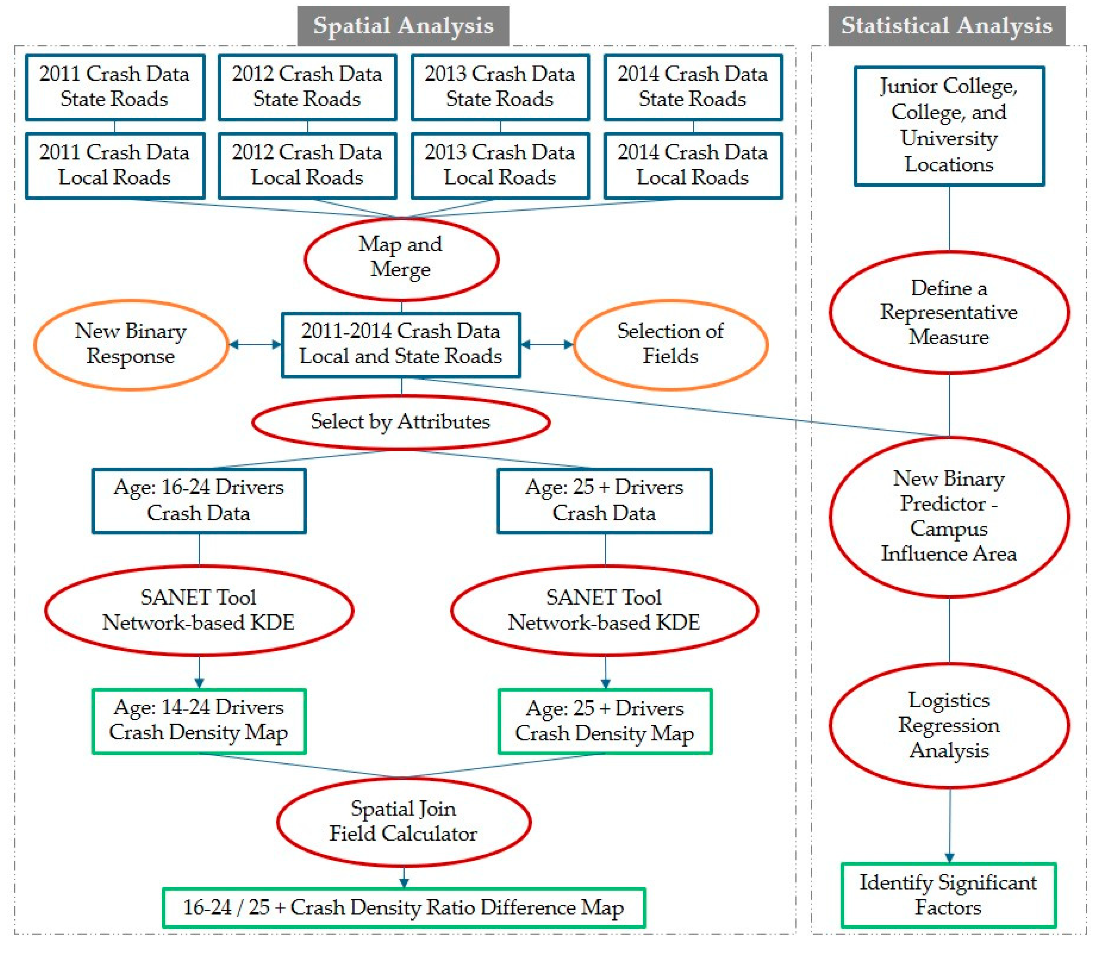
Several studies have used statistical analyses to investigate the predictor variables that could significantly affect roadway crashes and their severity [49,50]. In the literature, several studies have shown that different environmental, roadway- and driver-related predictor variables have different effects on the probability of crash involvement with regard to various age groups [51]. Scanning the literature, many studies have applied logistic regression in the context of crash studies. For example, Kong and Yang used logistic regression to investigate the relationship between speed and pedestrian casualty in vehicle-pedestrian collisions in China [52]. Elsewhere, Fitzpatrick et al. developed logistic regression models to identify which crashes truly were or were not considered as speeding-related crashes, given the crash narratives [53]. More broadly, logistic regression models have been used widely as the binary choice models in the literature, such as in cases of choices between the probability of crash occurrence and interacting predictors [54,55]. Ye and Lord [56] conducted a Monte-Carlo approach based on simulated and observed crash data to compare three different models, including multinomial logit, ordered probit, and mixed logit models to identify the required sample size for crash severity modeling. The results indicated that the mixed logit model and the ordered probit model required the highest and lowest sample size, respectively [56]. Additionally, Alam and Spainhour [2] implemented a binary logit model in order to investigate the association between at-fault drivers’ age with fatal crashes on highways and state roadways in Florida. The findings indicated that the probability of fatal crashes is higher for younger (≤24 years) and older drivers (65–74 and ≥75) than other age cohorts. Recently, Se et al. [57] employed the hierarchical binary logit technique to compare driver injury severity and found that roadside safety features (guardrails) significantly reduce fatal crashes among young drivers, but they did not expand the result around university campus areas specifically. Ulak et al. [48] also applied a three-step spatial analysis on three urban counties in northwest Florida to investigate crashes involving aging drivers. They developed a statistical analysis to identify the predictor variables that are statistically significant in crashes involving aging drivers. The results of this study revealed different spatial and temporal patterns for aging-involved crashes compared to other age groups. However, none of these studies specifically focused on young-driver-involved crashes that occurred in the proximity of university areas using GIS-based models and statistical methods.

3. Methodology

The main objective of this research is to develop a GIS-based methodology that can be used to spatially analyze young-driver-involved roadway crashes and determine if university campus locations are prone to more young-driver-involved crashes or not. The paper focuses specifically on the crashes that involve youth populations in order to systematically determine the most hazardous locations associated with those crashes. By the hazardous location analysis, we mean identifying the youth population-involved hot spots and crash clusters on the given roadway network and evaluating the hypothesis that roadways around universities are among the highest-risk areas with respect to young-driver crash densities in the selected counties with distinguishing college-oriented characteristics. Moreover, logistic regression model findings statistically confirm the visual conclusions obtained by GIS in the following sections. A descriptive flowchart displaying the overall spatial-statistical analysis methodology is provided in Figure 1. This methodology was applied to three urban counties in Florida: Alachua, Leon, and Duval. Leon and Alachua counties are homes to two college towns, Tallahassee and Gainesville, respectively, whereas Duval County is one of the most highly populated counties of Florida, with a high university student population. We intend to assess how different types of counties have impacted young-driver crash density patterns.

One of the most common methodologies used for a GIS-based spatial clustering analysis is kernel density estimation (KDE). KDE is used to identify the density of high crash occurrence locations called hotspots [45]. There are two major approaches to conduct the KDE analysis: planar Euclidean distance (ED)- and roadway network distance (RND)-based. The planar method utilizes the Euclidean distances between crash points, whereas the latter one utilizes the actual roadway network distance. At a higher level, when looking at a whole state or county, for example, it may be appropriate to use planar methods generally. However, at a local level, while looking at specific corridors and intersections, the ED method will identify all the roadways and intersections that reside in the peak density region as ‘high crash’ risk locations. This is critical because it may cause the following problems: (a) Overestimation: Some roadways that do not actually possess high risk are shown to be as such, (b) Underestimation: Because multiple roadways are shown as critical locations rather than the actual roadways that have high crash risk, one may not give the needed attention to the actual high-risk locations. The SANET toolbox, which is based on roadway network-based distance calculations, solves the overestimation and underestimation problems associated with the ED kernel density estimation approach and therefore provides more accurate hotspots at a local level.

The selection of bandwidth values is also critical for the KDE approaches. This is mainly owing to the fact that considering extremely small bandwidths might discard the critical clusters by diminishing connections between points, whereas very large bandwidths might fail to identify local clusters by averaging out the effect of closely connected points [58]. Hence, as an example, bandwidths can be selected based on trial-and-error for the ED approach [59]. A research study conducted by Okabe et al. suggests a bandwidth ranged from 100–300 m. for applying the network-based KDE, especially in urban areas. Therefore, in this paper, a 200 m. bandwidth has been selected for both ED and RND approaches based on trial-and-error within the range provided in previous research for urban networks [60]. Moreover, the SANET needs another input named cell-width value, which was taken as equal to 20 [47] (one-tenth of the bandwidth).

In addition, we applied a crash Density Ratio Difference (DRD) measure to evaluate the difference between normalized crash intensity ratios for two age groups: 16–24 and 25 and over. The DRD is a useful index to identify and investigate hotspots, which was developed in a research conducted by Ulak et al. in 2017 [48]. This comparative crash density analysis was conducted to evaluate the spatial patterns of crashes that involve the youth population and compared hotspots between different age groups. In this paper, DRD represents the difference between the maxima-normalized crash densities for the following crash drivers: 16–24 and 25 and over. The formula of DRD is shown in Equation (1).

$${\mathrm{DRD}}_{\mathrm{ij}}=\frac{{\mathrm{D}}_{\mathrm{i}}}{\max \left({\mathrm{D}}_{\mathrm{i}}\right)}-\frac{{\mathrm{D}}_{\mathrm{j}}}{\max \left({\mathrm{D}}_{\mathrm{j}}\right)}$$

(1)

where DRD_ij is the density ratio difference between the compared maps I and j, whereas Di and D_j are the density values of the corresponding roadway sections, and max (D_i) and max (D_j) are the maximum crash density values of the compared maps, respectively. Based on this approach, the highest value of normalized density for each age group is equal to 1, whereas the lowest value of normalized density is equal to 0. Based on the calculation of normalized crash densities, the crash density map of the 16–24 (map i) age group is subtracted from the crash density map of 25 and over (map j) drivers individually. Therefore, the DRD index reveals the relatively different locations in the area, which provides even more explicit visual results in terms of geo-spatial differences between the two different age groups.

Note that there is an extensive amount of research literature available on the generalized linear regression models. Logistic regression, which is also known as logit model or logit regression, is used as a statistical analysis to predict the probability of an event happening given the available data. Logit regression is a suitable regression model when the dependent variable is binary [61]. In this paper, we present three separate logistic regression models for each county in order to estimate the effects of these factors on young-driver-involved crashes and test their level of significance. The model includes a binary predictor variable that indicates whether a crash occurred around university campuses or not. To define this variable, we added a binary attribute to the crash dataset, coded as 1, indicating a crash occurrence within a 5-mile buffer around campus, and zero for otherwise. The response variable (a crash involving a young driver or not) utilized in the model is also binary; hence, a binary choice model was developed in this study. In order to estimate the coefficients of the predictor variables of the logit model, we maximized the following log-likelihood function:

$$\mathrm{lnL}\left(\mathsf{\delta }\mathsf{\beta }\right)={{\displaystyle \sum }}_{\mathrm{i}=1}^{\mathrm{n}}\left\{{\mathrm{Y}}_{\mathrm{i}}*\left[\mathsf{\psi }\left({\mathrm{X}}_{\mathrm{i}}\mathsf{\beta }\right)\right]+\left(1-{\mathrm{Y}}_{\mathrm{i}}\right)*\left[1-\mathsf{\psi }\left({\mathrm{X}}_{\mathrm{i}}\mathsf{\beta }\right)\right]\right\}$$

(2)

where Y_i is the binary response variable (0 or 1) that denotes the occurrence of a young-driver crash, X_i is the row vector for the values of the predictor variables for ith observation, $\mathsf{\beta }$ is the vector of coefficients of the predictor variables, n is the number of data points (crash or non-crash) observed in the study region, and $\mathsf{\psi }\left({\mathrm{X}}_{\mathrm{i}}\mathsf{\beta }\right)$ is the cumulative distribution function of the logistic function. In this study, the response variable Y_i is equal to 1 if the crash involved a young driver, or 0 otherwise.

In the current study, a subset of predictor variables has been considered based on the Pearson correlation coefficients, forward selection method, literature review, and authors’ prior knowledge to develop the logistic regression models for all three counties, namely Alachua, Duval, and Leon.

Table 1. Description of predictor variables.

Predictor Variable	Description
Estimated Vehicle Speed (mph)	The vehicle’s speed at the time of the crash
AADT (Divided by 1000)	Average Annual Daily Traffic divided by 1000
Weekend	The crash occurred on Friday, Saturday, or Sunday
At Peak Hours	The crash occurred during peak hours (6–9 a.m. & 4–7 p.m.)
Alcohol-Drug Abuse	One or more drivers were under the influence of alcohol/drugs
Intersection Presence	Intersection involvement for the crash
Weather Conditions	The crash has not occurred during clear weather conditions
Light Conditions	The crash has not occurred during daylight conditions
Speeding Violation	Speeding involvement for the crash
Aggressive Driving	Aggressive driving by one or more of the drivers
Fatality or Incapacitating Injury	Fatality or Incapacitating injury has occurred
Distracted Driver	One or more drivers were distracted at the time of the crash
Single Driver	Single-Driver crash (No passenger)
Within University Area	The crash occurred within a 5-mile buffer around the university

lists the predictor variables along with their descriptions. The fitted logistic regression models for the three counties and the discussion of these results is provided in the Results Section. The glm command in R has been used to fit the logistic regression models.

In Table 1, the first two predictor variables are continuous, and the others are defined as binary variables, meaning that 1 stands for “Yes” and 0 otherwise.

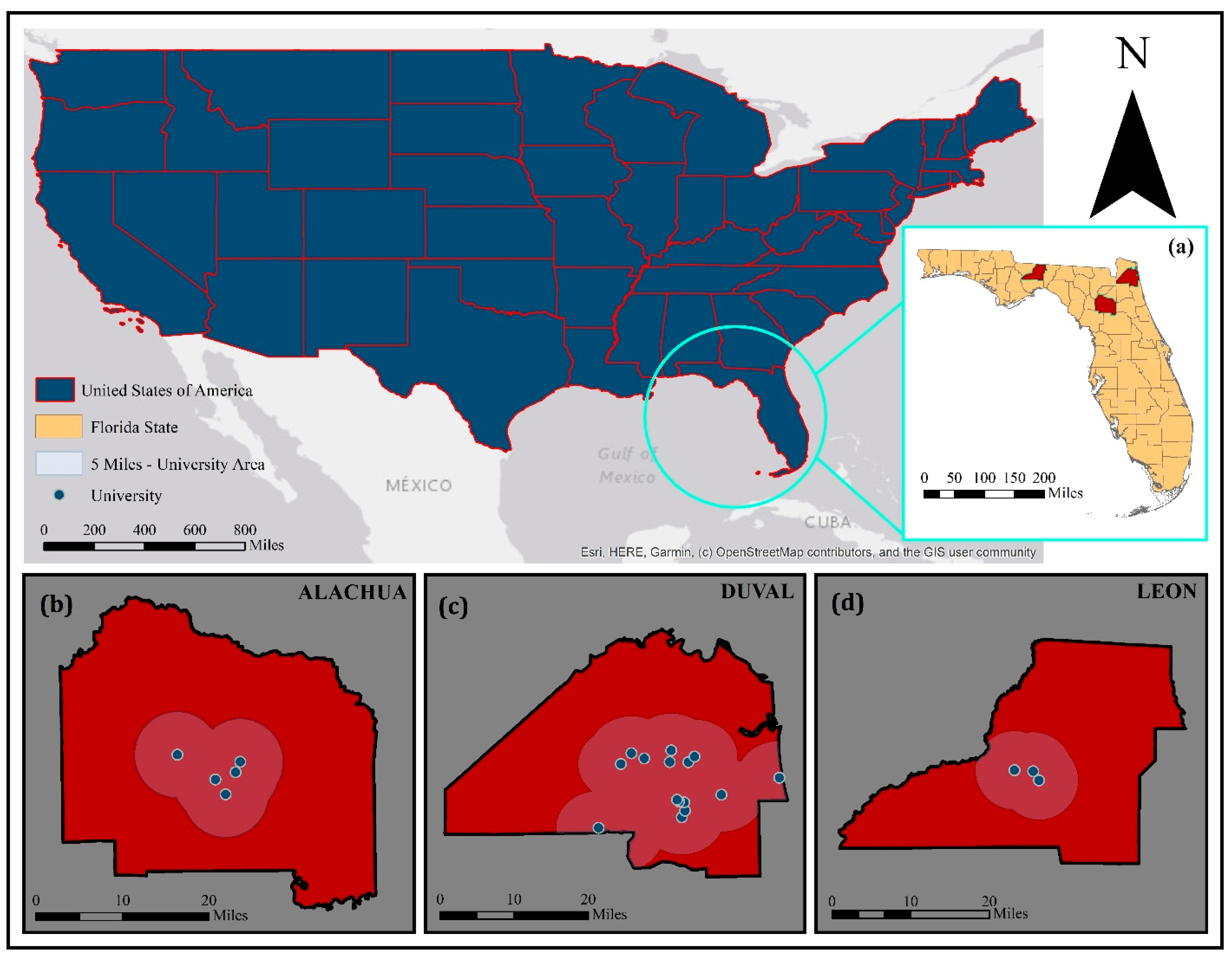
4. Study Area and Data Description

This research intends to examine the correlating factors associated with young-driver-involved crashes that occurred around campuses of junior colleges, colleges, universities, or professional schools. To follow this purpose, we focus on the youth-age (16–24) drivers involved in crashes occurring in the whole state of Florida, and three selected Florida counties namely Alachua, Duval, and Leon, in detail. The Florida Department of Motor Vehicles (DMV) issues a restricted license to teenagers between 15 and 17 once they complete the required courses and tests [62]. A teenager must have a learner permit for one year while practicing their driving skills with an adult. After 12 months with a learner permit, he/she can then take the driving test to obtain a full Florida driver’s license [62]. In this study, therefore, we screened the crashes where the driver was aged between 16 to 24. We will use the term “young-driver-involved crashes” to represent this type of crash in this paper. The above-mentioned age group is associated with the youth population who attend junior colleges, colleges, universities, or professional schools based on National Center for Education Statistics (NCES) suggestions [63].

According to the U.S. Census estimates, as of 2019, Duval County is the seventh most populated county in Florida and contain 15 universities and other higher education institutions. Alachua and Leon County, on the other hand, are considered mid-size counties based on their populations [16]. The crash data is composed of points dispersed along the roadway network, and each point represents a vehicle crash with the associated driver information. This dataset was obtained from the FDOT Safety Office in the format of GIS shapefiles and their respective databases and includes 4 years of data from 2011 to 2014 [64]. These shapefiles were extracted and mapped onto the GIS using the longitudes and latitudes of each crash data point. Roadway network, on the other hand, was obtained from the TIGER Geodatabase of the U.S. Census Bureau [16].

Table 2. Overview of Crash data in Florida Counties between 2011 and 2014.

Year
		2011	2012	2013	2014	Total
Local Roadway	Florida	100,220	113,514	133,605	157,229	504,568
	Alachua	1340	1396	1346	1255	5337
	Duval	3731	7888	8827	8567	29,013
	Leon	2405	2387	2611	2774	10,177
Highway System	Florida	145,517	169,310	194,456	214,968	724,251
	Alachua	3473	3568	3812	3301	14,154
	Duval	8269	16,723	17,584	17,279	59,855
	Leon	2756	2797	2934	3205	11,692

shows the number of crashes for the whole state as well as each county separately. It should be mentioned that separate datasets including local roadway and highway system crashes were merged in order to obtain one aggregated crash dataset that includes all the crashes that occurred during the years from 2011 to 2014.

Figure 2 illustrates the overview of the study area, including university locations in each county. Leon and Alachua counties are home to two college towns, Tallahassee and Gainesville, respectively, whereas Duval County is one of the most highly populated counties of Florida, with a high university student population. Alachua and Leon are among the highest college-oriented counties, with a great number of students enrolled at junior colleges, colleges, universities, and professional schools (See

Table 3. Overview of the Universities, and Number of Crashes around University.

County	Total Population	Total # of Crashes	Total # of Young-Driver-Involved Crashes (% to Total)	Total # of Young-Driver-Involved Crashes Around the University (% to Young-Driver-Involved Crashes)	Junior Colleges, Colleges, Universities, and Professional Schools	Enrollment
Alachua	269,000	19,491	8177 (42%)	7191 (88%)	University of Florida	51,475
					Santa Fe College	14,796
					Dragon Rises College of Oriental Medicine	36
					City College Branch Campus	272
					Academy for Five Element Acupuncture	32
Duval	957,000	88,868	27,930 (31%)	24,365 (87%)	University of Phoenix-North Florida Campus	1126
					University of North Florida	14,982
					Trinity Baptist College	300
					Stenotype Institute of Jacksonville Inc.	293
					Remington College—Jacksonville Campus	Online
					Jones College—Jacksonville	558
					Jacksonville University	3418
					ITT Technical Institute—Jacksonville	552
					Heritage Institute—Jacksonville	388
					Florida Technical College of Jacksonville Inc.	204
					Florida Community College at Jacksonville	25,686
					Florida Coastal School of Law	1498
					Everest University—Jacksonville	438
					Edward Waters College	840
					Concorde Career Institute	587
Leon	293,000	21,869	8833 (40%)	7166 (81%)	Tallahassee Community College	14,048
					Florida State University	38,717
					Florida Agricultural and Mechanical University	11,672
					Flagler College—Tallahassee	454

All # signs indicate numbers.

).

Moreover, in Table 3, we observe that a considerable percentage of drivers involved in crashes that occurred in these counties are those that are between the ages of 16 and 24, as expected. Using the GIS query tool, crash data for the age group of 16–24 and 25 and over were separated. Note that crash data include the required information associated with drivers involved in a crash. These data do not include crashes occurring at parking lots, on private property, and on private roadways. The roadway network, on the other hand, is obtained from the TIGER Geodatabase of the Census Bureau [16]. We also consider the locations of all junior colleges, colleges, universities, and professional schools within three selected counties in Florida, obtained from the U.S. Geological Survey [65].

This study examined the crash spot-residence location distances based on the occupant residential ZIP code centroid. The results of this study imply that if there is a crash around a facility, it is more likely that the crash is closer to the residential ZIP code of the crash occupants. We focus on those crashes that are in the vicinity of the campus locations (selected based on a 5-mile buffer). Based on previous studies, the 5-mile buffer zone radius is selected as a reasonable proxy for a typical trip length traveling by a personal vehicle [66]. Moreover, a 5-mile radius is roughly consistent with the assumption of a 15-min driving distance from the crash location, accounting for the effects of traffic signals and possible delays on roadways depending on the roadway and traffic characteristics [13]. For these reasons, a 5-mile radius is selected as a representative measure for the crash locations in the three studied counties. Based on Table 3, it is also worth mentioning that a noticeable percentage (>80%) of young-driver-involved crashes occurred around universities within the selected 5-mile buffer.

5. Results

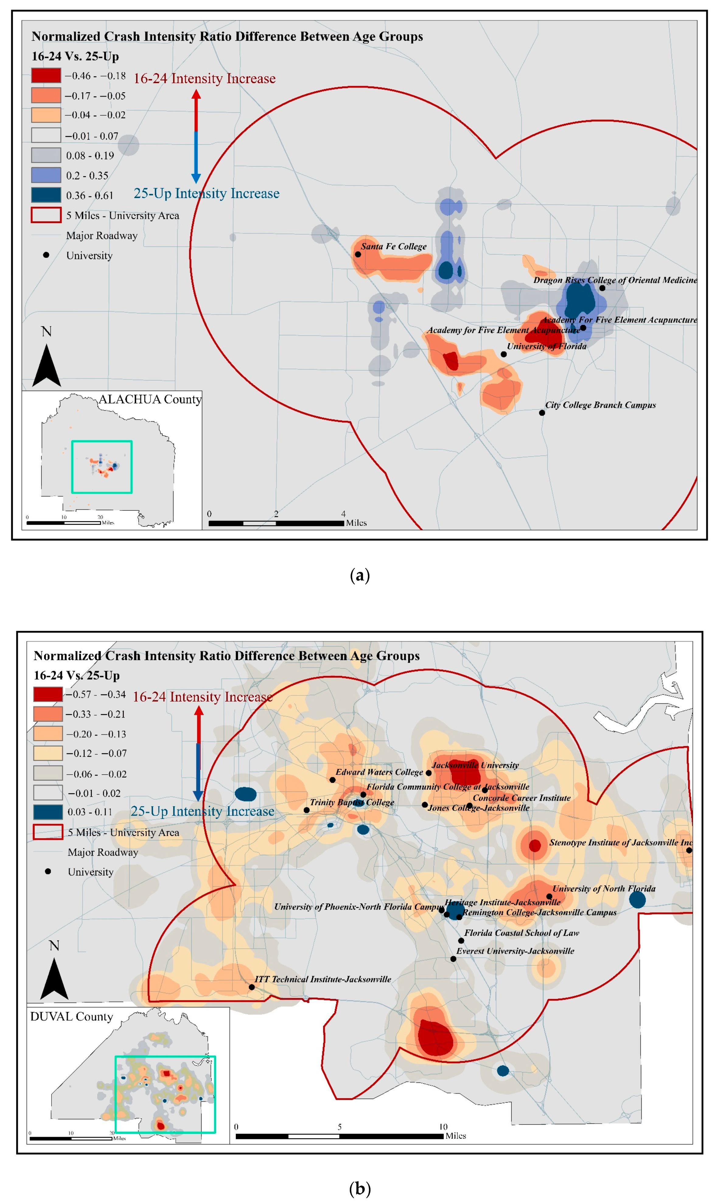
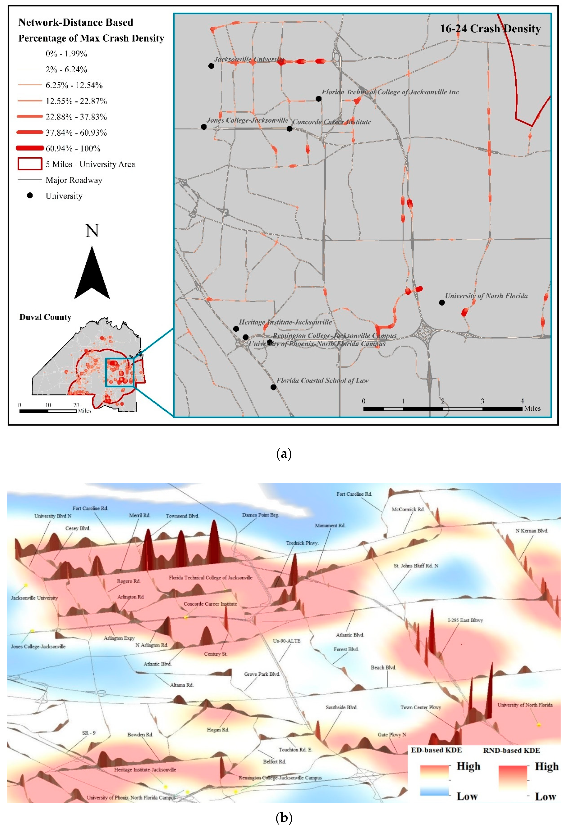
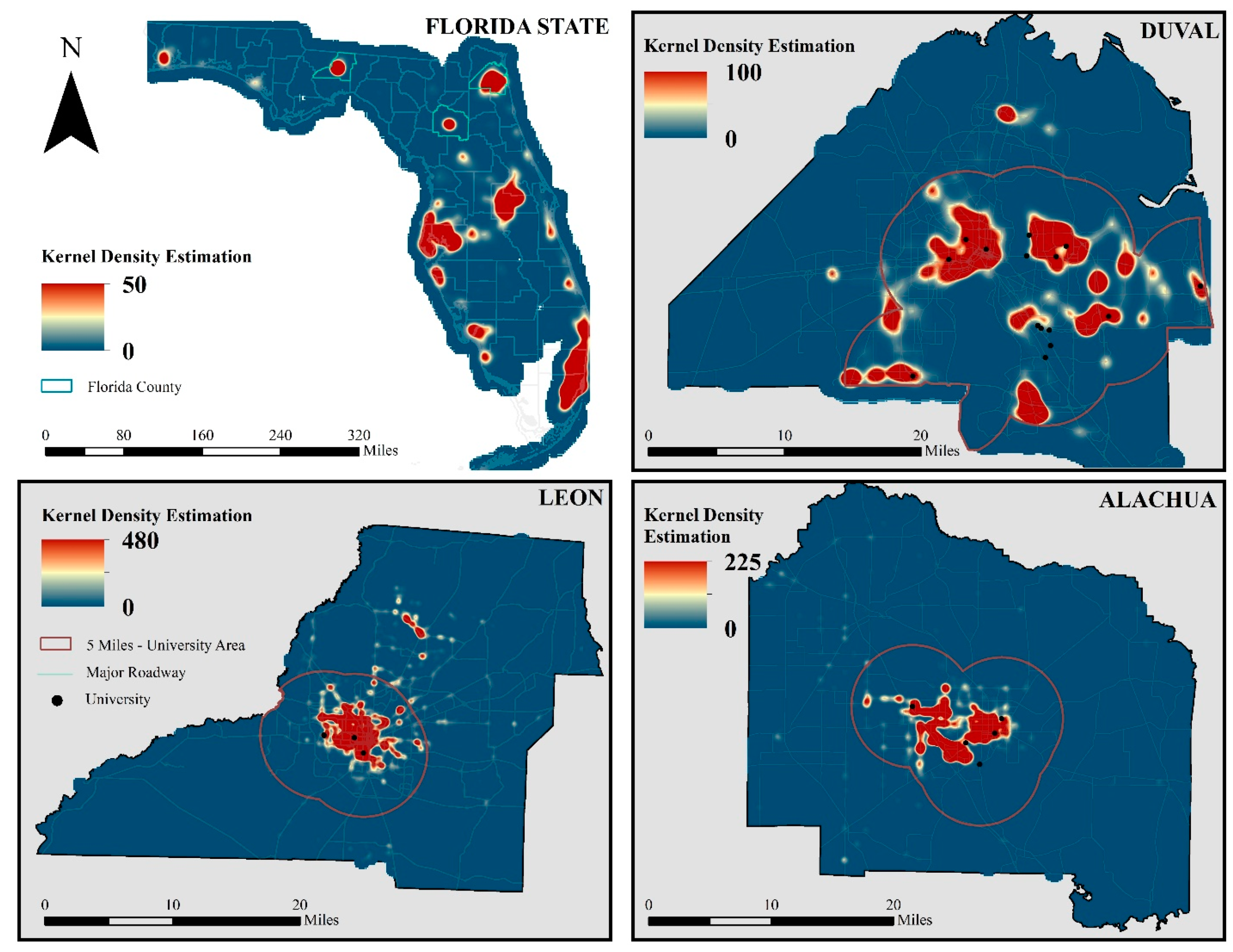
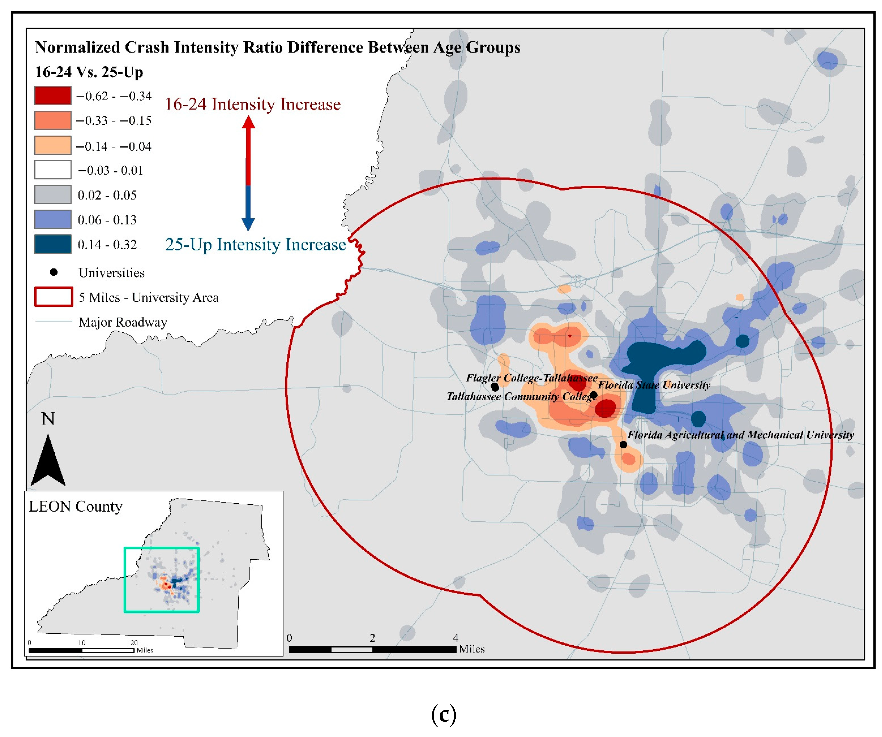
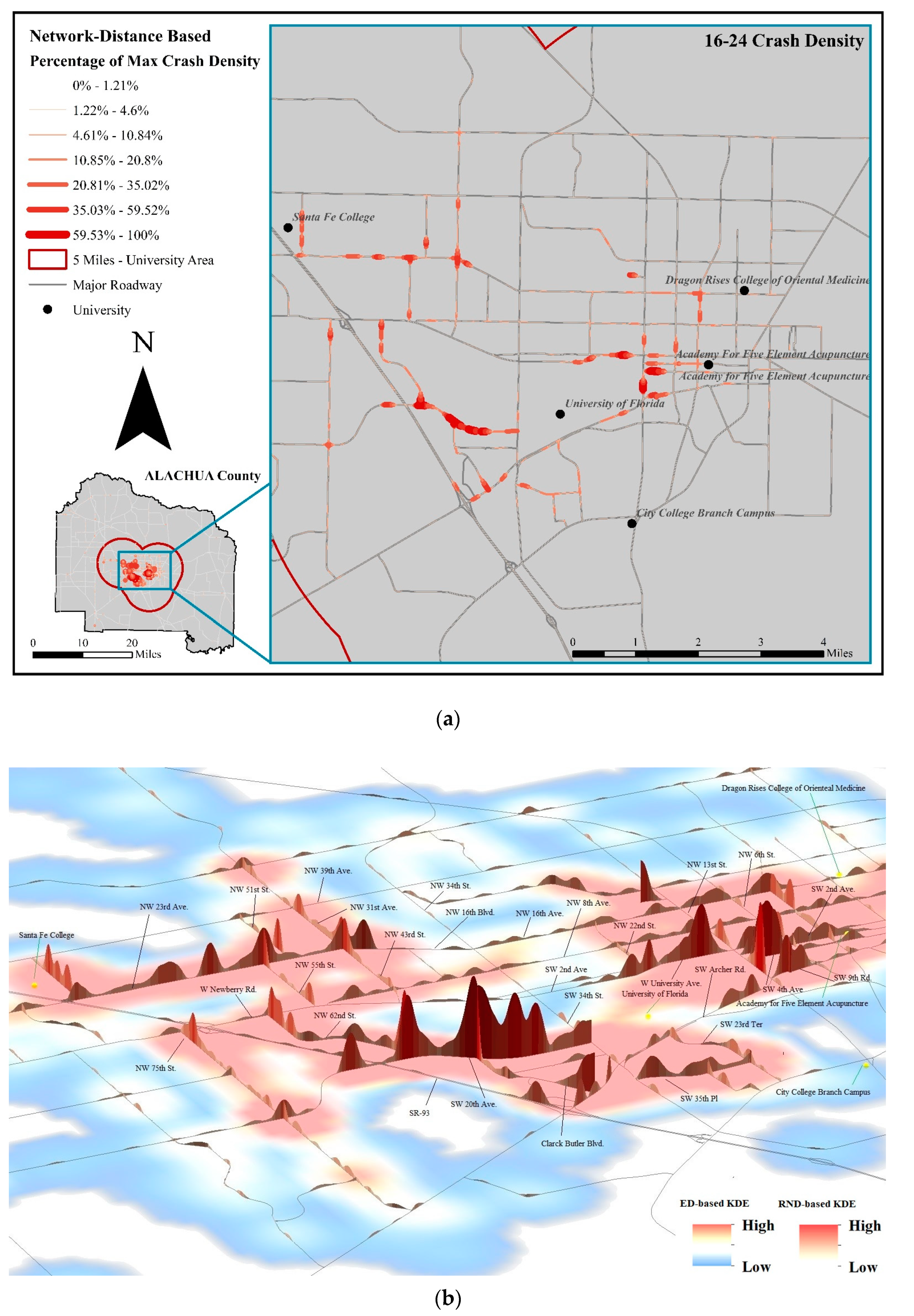
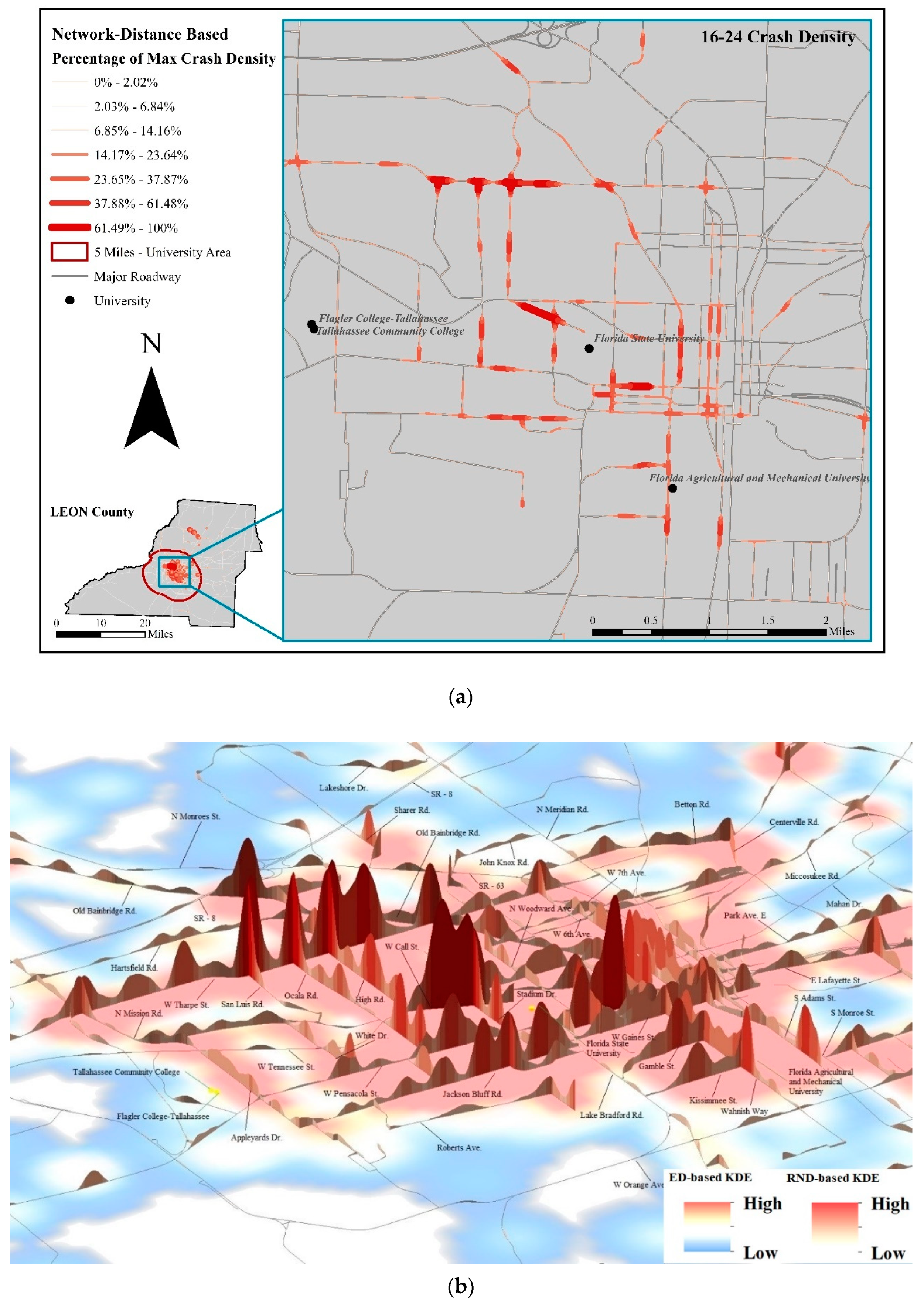
5.1. GIS-Based Visual Illustrations

The kernel density estimates of the crash counts of the three counties were computed in ArcGIS and the SANET toolbox. Figure 3 shows the results obtained from the ED application for the State of Florida as well as the selected counties. Note that the dark red areas in Figure 3 indicate the high-crash-risk locations around university campuses with respect to young-driver-involved crashes. For the whole state, it is clear that many metropolitan regions have higher crashes involving young people. This study, on the other hand, focuses on two counties that include college towns (Tallahassee and Gainesville), namely Leon and Alachua counties, where high-risk locations are clustered around the universities (See Figure 3 and Figure 4). The third county selected is Duval County, which is a larger metropolitan area including the City of Jacksonville. Based on this county selection, at the county level, the DRD methodology was applied using the ED approach, and the results can be seen in Figure 4.

Based on Figure 4, the normalized crash intensity ratio differences between those aged 16–24 and those that are over 25 seem to occur mostly in the vicinity of the University of Florida and Florida State University in Leon and Alachua counties, respectively. The dark red areas indicate that the 16–24 age group crash intensities increase around universities, particularly in Leon County. In Duval County, on the other hand, there are no distinguished patterns, possibly due to the higher urbanization of the region. The hotspots shown as dark red are located to the north of the 5-miles university area (including Jacksonville University, Florida Technical College of Jacksonville, Concorde Career Institute, and Jones College-Jacksonville) in Duval County. There are no clear differences between crashes involving 16–24 vs. the 25 and up populations around the University of North Florida and Florida Community College. This may be linked to the high population and urbanization of the city itself.

The ED approach has been implemented at the county level in Figure 3. However, in order to estimate the extent of the high-risk locations more accurately at a local level, the RND approach is applied to those regions around the universities that seem to pose a high risk for youth populations (see Figure 5, Figure 6 and Figure 7). Based on what is shown in Figure 3, at a state level, it may be appropriate to use ED-based methods. However, at a local level, while looking at specific corridors and intersections, the ED method will identify all the roadways and intersections that reside in the peak density region as hotspot locations. This is critical because it may cause overestimation or underestimation. Therefore, the exact hotspot locations that require an appropriate safety improvement countermeasure remain unidentified. The proposed two-stage approach is aimed at achieving computational efficiency. This is achieved through the SANET method and is shown in Figure 5a, Figure 6a and Figure 7a. Taking this approach, it becomes possible to detect the roadways that have a high number of young-driver-involved crashes where every distance between the crashes is calculated based on the actual roadway (network) distance. The 3D maps of Figure 5b, Figure 6b and Figure 7b were created based on the SANET method and represent those distributions of the RND approach. The 3D maps of Figure 5b, Figure 6b and Figure 7b present the ED-based KDE displayed as a blue to a red color ramp on the plane, and the RND-based KDE outputs have been plotted above the ED-based KDE in perspective 3D view in white to the red color ramp.

As stated earlier, Figure 3 represents the ED-based results for Alachua, Duval, and Leon counties, and shows the crash hotspots located in the 5-mile buffer around the university campuses. The RND approach, represented in Figure 5, Figure 6 and Figure 7, on the other hand, enables us to identify the exact locations of the most critical hotpot corridors. As such, the drawbacks of the planar KDE approach are more visible in the 3D visualization of crash density maps of the counties. For example, some parts of the university region, which is shown as a critical hotspot in the ED-based maps in Figure 3, do not have the highest peak (highest crash risk) in the 3D maps created using the RND approach (Figure 5 through Figure 7).

With a focus on Figure 5, considering Alachua County, the RND approach does not show any critical hotspots in some parts of NW 31st Ave., W Newberry Rd., SW 34th St., or NW 6th St., which are identified as being important by the ED approach. This indicates that ED-based KDE overestimates the crash density along these roadways. Although this may not be entirely visible from the 2D maps, they are typically identifiable by the high surface peaks in the three-dimensional (3D) view of crashes (Figure 5).

Similarly, with regard to the results presented in Figure 3, almost the entire area around Florida Technical College of Jacksonville and Concorde Career Institute appear to be critical due to their dark red color; however, the whole area is not actually a hotspot, but rather certain roadways have higher crash rates than others in that particular area. This is more precisely shown through using the SANET results shown in Figure 6. Other similar examples include Cesey Blvd., Rogero Rd., and Townsend Blvd (Figure 6).

The same overestimation is observed in Leon County (Figure 7). Although the whole area around Florida State University is shown in dark red and identified as hotspots in the ED approach, some segments are critical hotspots identified by the RND approach, such as W Call St. intersection with Stadium Dr. N Woodward Ave., S Adams St., and W 7th Ave., on the other hand, are not as critical as W Call St. intersection with Stadium Dr. based on the RND approach. However, those locations are also shown to possess a high risk based on the ED approach (Figure 7). Thus, RND-based KDE leads us to a more detailed assessment of young-driver-involved crashes, and this approach allows us to observe high-crash-risk locations more clearly and accurately.

Based on analyzing the high peaks in Alachua County in Figure 5b, there appears to be two major hotspots around the university area: the intersection of SW 20th Ave and NW 62nd St. and SW 20th Ave and W. University Ave. These locations are in the vicinity of the University of Florida. Similarly, the intersection of W Tharpe St. and San Luis Rd., the intersection of W Tharpe St. and Ocala Rd., and the intersection of W Tharpe St. and High Rd. in Leon County are among the most critical hotspot associated with youth-involved crashes (Figure 7b). Figure 6b also clearly shows that the highest young-driver crash density in Duval County is found at the Townsend Blvd. and Merril Rd. intersection.

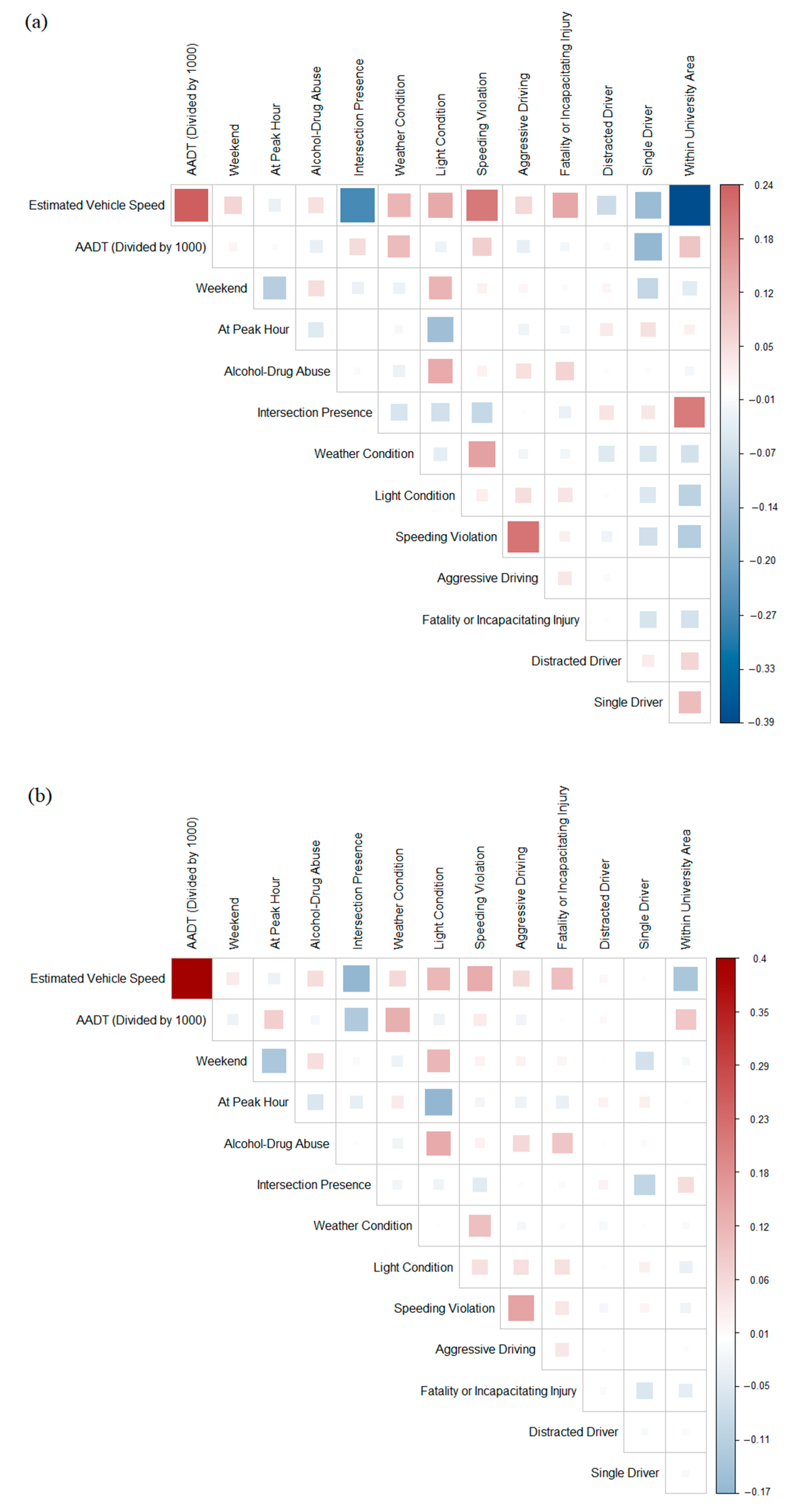
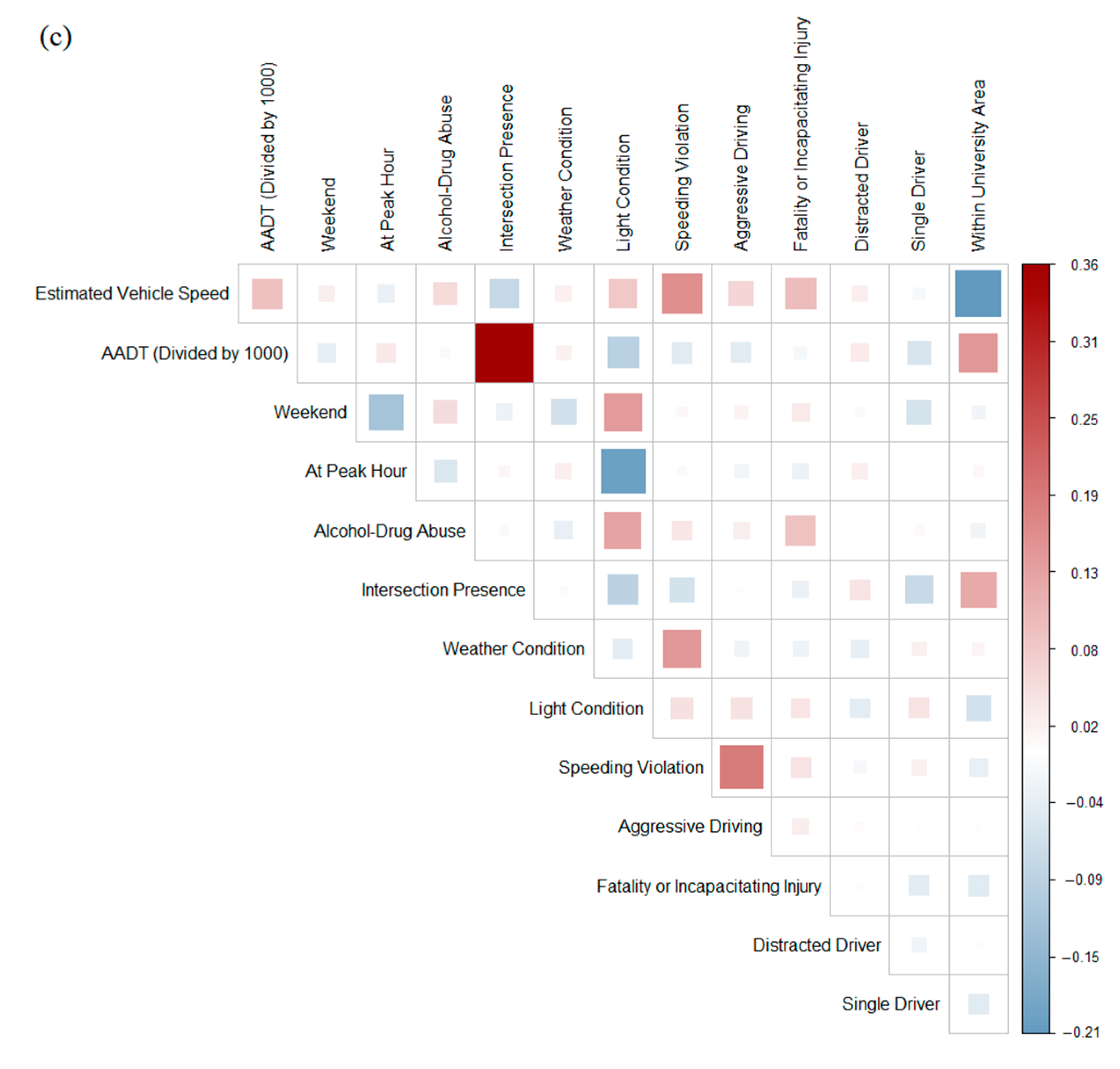
5.2. Regression Analysis

In order to develop the logistic regression models, we considered a subset of predictor variables for the regression analysis, selected based on the Pearson correlation coefficients (see Figure 8), literature review, and the authors’ prior knowledge. This approach enables us to remove the ones with the high correlation value to develop a more accurate regression model and avoid multicollinearity and inflation while predicting the probability of occurrence of young-driver-involved crashes. The correlation matrices shown in Figure 8 yield the results needed to examine the influence of predictor variables on each other. Based on the correlation matrix shown for Duval County (Figure 8b), there is a high correlation between “Estimated Vehicle Speed” and “Average Annual Daily Traffic” that leads to collinearity. This indicates that considering both predictor variables in logistic regression models will cause some regression coefficients to have a wrong sign and inflate the variance of the estimated regression coefficients. Thus, we removed the “Estimated Vehicle Speed” from the model for Duval County. We also developed another logistic regression model with “Estimated Vehicle Speed” and without “AADT” to check their influence on the results.

The results of statistical analyses for the selected three counties, namely Alachua, Duval, and Leon, are provided in

Table 4. Logistic regression analysis results, (a) Alachua County, (b) Duval County, (c) Leon County.

Regressors	Alachua County				Duval County				Leon County
	β	SE	p	VIF	β	SE	p	VIF	β	SE	p	VIF
Intercept	−1.319	0.060	$\approx 0$		−0.865	0.026	$\approx 0$		−0.933	0.053	$\approx 0$
Estimated Vehicle Speed	0.005	0.001	$\approx 0$	1.41					0.016	0.001	$\approx 0$	1.13
AADT/1000	0.002	0.001	0.04	1.16	0.002	0.000	$\approx 0$	1.05	−0.002	0.001	0.02	1.20
Weekend					−0.031	0.015	0.04	1.03
At Peak Hour					0.047	0.015	$\approx 0$	1.05	−0.093	0.031	0.01	1.04
Alcohol/Drug Abuse	0.393	0.109	$\approx 0$	1.01					0.206	0.124	0.09	1.03
Intersection Presence	0.185	0.031	$\approx 0$	1.10	0.115	0.015	$\approx 0$	1.04	0.199	0.031	$\approx 0$	1.18
Weather Condition	0.057	0.032	0.07	1.03	0.058	0.015	$\approx 0$	1.03
Light Condition					0.053	0.016	$\approx 0$	1.05	−0.169	0.031	$\approx 0$	1.08
Speeding Violation					0.373	0.050	$\approx 0$	1.04	0.532	0.070	$\approx 0$	1.07
Aggressive Driving	−0.748	0.168	$\approx 0$	1.01	0.179	0.085	0.03	1.03	−0.238	0.120	0.05	1.04
Fatality/Incapacitating	−0.215	0.073	$\approx 0$	1.03	−0.114	0.039	$\approx 0$	1.01	−0.331	0.083	$\approx 0$	1.02
Distracted Driver	0.387	0.039	$\approx 0$	1.01	0.351	0.021	$\approx 0$	1.00	0.477	0.040	$\approx 0$	1.00
Single Driver	0.068	0.030	0.02	1.05	−0.337	0.015	$\approx 0$	1.02	−0.358	0.029	$\approx 0$	1.01
Within University Area	0.718	0.046	$\approx 0$	1.24	0.067	0.022	0.002	1.02	0.371	0.037	$\approx 0$	1.09
	N: 19,491, df: 19,480				N: 88,868, df: 88,855				N: 21,869, df: 21,856
	$\mathsf{\chi }2=526,p\approx 0$				$\mathsf{\chi }2=1130,p\approx 0$				$\mathsf{\chi }2=893,p\approx 0$

Generalized linear regression model: logit (y) ~ 1 + x1 + x2 + x3 + x4 + x5 + x6 + x7 + x8 + x9 + x10 + x11 + x12 + x13 + x14. y ~ Probability of a crash to involve a young driver (16–24). Binary variables: “Weekend” (1: Weekend, 0: Weekday), “At Peak Hour” (1: Yes, 0: No), “Alcohol/Drug Abuse” (1: Yes, 0: No), “Intersection Presence” (1: Yes, 0: No), “Weather Condition” (1: Otherwise, 0: Clear), “Light Condition” (1: Otherwise, 0: Daylight), “Speeding Violation” (1: Yes, 0: No), “Aggressive Driving” (1: Otherwise, 0: Clear), “Fatality or Incapacitating injury” (1: Yes, 0: No), “Distracted Driver” (1: Yes, 0: No), “Single Driver” (1: Yes, 0: No), “Within University Area 5-mile buffer zone” (1: Yes, 0: No). Continuous Variables: “Estimated Vehicle Speed”, “AADT”. Abbreviations: β: estimated coefficient, SE: standard error, p: p-value, N: number of observations, df: degrees of freedom, χ²: Chi2 statistics vs. constant model. Note: The models merely include the independent variables with at least a 90 percent level of significance.

. In the table, the “β” coefficients show the positive or negative contribution of predictor variables on the response variable, relatively. “SE” values, which stand for Standard Error, estimate the standard deviation of the coefficients in the model. That is, it measures the precision of the model. Additionally, “p” values reveal the significance level of different predictor variables on the binary response variable, and these values have been used to examine whether a predictor variable has significance at 90% or higher per the logistic regression model used for each county. It is worth mentioning that the predictors have been added to the models based on a step forward selection method one at a time [61]. Variable Inflation Factor (VIF) has also been examined to ensure the selected predictors are not mutually correlated and hence do not cause inflation of the estimation uncertainty. The forward selection approach along with VIFs allowed us to keep all the selected crash-related factors in the logistic regression models and distinguish the differences between the associated significant levels for each county.

We found that “Estimated Vehicle Speed” has a positive effect on the response variable at a 99% level of significance, similar to the other two counties. This indicates that the higher estimated vehicle speed increases the probability of youth involvement in crashes. It is also worth mentioning that there are negative correlations between “Estimated Vehicle Speed” and “Within University Area” for all these three counties (See Figure 8). That is, the vehicles involved in the crashes occurring around campus areas (within 5-miles buffer) have lower speed estimation at the time of crash, mainly due to the lower speed limit in these areas. Thus, it could be concluded that the lower speed limits around campus area do not necessarily prevent young-driver crash occurrence despite their effectiveness in decreasing vehicle speed. Note that all three logistic regression models are thoroughly checked for possible multicollinearity issues between predictors based on the VIF and correlation matrices provided in Figure 8.

Statistical results obtained by logistic regression models also reveal that “Distracted Driver”, “Intersection Presence”, and “Within University Area” variables have statistically significant increasing effects on the probability of young-driver-involved crashes for all these counties. The positive estimated coefficient for “intersection presence” indicates higher young-driver crash probabilities at intersections. Furthermore, Figure 8 illustrates positive correlations between “Within University Area” and “Intersection Presence” variables in all three counties. This shows that most of the problematic intersections are located around universities. These statistical findings confirm the soundness of results obtained by the RND-based KDE method that illustrated those intersections in dark red as hotspot areas with noticeable young-driver crash densities (see Figure 5 through Figure 7). Based on the crash data considered in the current study, 10,305 crashes occurred at intersections in Alachua County. Among these, 4623 crashes were young-driver-involved crashes, which is approximately equal to 45% of the total number of crashes occurring at intersections. It is also worth mentioning that, among the 1937 crashes occurring at intersections where the driver was distracted, 1015 (about 52%) of them involved young drivers. Duval County and Leon County also follow a similar pattern (

Table 5. Number of crashes involving intersection and distracted driver.

County	Total # of Crash	Total # of Intersection Involvement Crash	Young-Driver Intersection Crash	Total # of Distracted Driver at Intersection Involvement Crash	Distracted Young Driver at Intersection
Alachua	19,491	10,305 (53%)	4623 (45%)	1937 (10%)	1015 (52%)
Duval	88,868	36,476 (41%)	12,031 (33%)	5015 (6%)	1994 (40%)
Leon	21,869	9362 (43%)	4037 (43%)	1422 (7%)	742 (52%)

Note: Italic percentage values in parentheses indicate the percentage of the total number of crashes. Underlined values indicate the percentage of the number of crashes with specific characteristics. All # signs indicate numbers.

).

Note that other age group populations may also have relatively more crashes at intersections [67]; however, the current research reveals that those intersections located around university campuses are prone to more young-driver-involved crashes. This problem was also evidenced in research conducted by Kidando et al. in 2018, where the youth populations were found to have 85.1% of all crashes on intersections on the Mahan Corridor of Leon County [68]. Because redesigning a roadway intersection would be very costly to transportation agencies, it can be more appropriate to maintain and operate the current intersections in a better and smarter way, especially in regions that have high youth population activities, such as the counties studied in this paper. Some effective interventions, including installing speed humps and intelligent traffic video surveillance, a higher level of police enforcement, and higher penalties for speeding violations alongside enacting more strict regulations could be utilized around universities to reduce young-driver-involved crashes. Intelligent Transportation System (ITS)-based safety improvement strategies implementations have also been studied in previous research, and they have the potential to yield better signalization, signing, and communication through IT-based systems. For instance, the application of an interactive in-vehicle tool, namely a “riskometer”, can be used to enhance the safety of young drivers [69].

The noticeable percentage of distracted young drivers at intersections indicates that this issue needs urgent attention to prevent the occurrence of these crashes. The effects of state-of-the-art technologies to improve the attentiveness of young drivers while driving and provide them with modern onboard devices to avoid distraction have been studied [70,71,72]. For instance, the connected vehicle (CV) and driving assistance (DA) technologies have the ability to reduce 94% of crashes in the U.S. that are due to either human error or bad/wrong decisions [73]. These technologies include, but are not limited to, the following: lane departure warning (LDW), intersection movement assist (IMA), forward collision warning (FCW), and adaptive cruise control system (ACC). For example, FCW can mitigate approximately 17 to 70% of rear-end crashes [74], while LDW has the ability to reduce about 17 and 33% of crashes if the application is fully operational [75].

The “Weekend” variable has a large negative coefficient for Duval County, which indicates that the probability of occurrence of young-driver-involved crashes during the weekdays is higher in comparison to the one for weekends. However, this variable does not have a significant influence in Leon and Alachua Counties, mainly as a result of the uniform temporal distribution of crashes during a week due to the college-oriented nature of these counties. Logit regression models reveal that the “Alcohol/Drug Abuse” variable has a different pattern with regards to its significant positive impact on the probability of young-driver-involved crashes in Alachua and Leon counties. On the other hand, it is not statistically significant for Duval County. This shows that driving under the influence of alcohol or drugs significantly increases the probability of young-driver-involved crashes in Alachua and Leon counties. This variable for Duval County, which is noticeably higher than the other two counties, on the other hand, does not have a significant contribution to the regression model.

Table 6. Number of Distracted or DUI young drivers.

County	Total # of Crash	Youth Involved Crash	Total # of Alcohol/Drug Crash	Young-Driver Alcohol/Drug Crash	Total # of Distracted Driver	Young-Driver Distracted Driver
Alachua	19,491	8177 (42%)	328	147 (45%)	3366	1696 (50%)
Duval	88,868	27,930 (31%)	1350	413 (31%)	11,553	4436 (38%)
Leon	21,869	8833 (40%)	290	131 (45%)	2982	1522 (51%)

All # signs indicate numbers.

shows this insignificant impact, which could be due to the low percentage of alcohol/drug and young-driver-involved crashes to the total number of alcohol/drug crashes.

The “Aggressive Driving” predictor has a high level of significance in all three counties; however, it is worth mentioning that it has a different pattern for Duval County. That is, for Leon and Alachua counties, aggressive drivers do not belong to the 16–24 age group, and the “Aggressive Driving” factor has a decreasing effect on the probability of occurrence of young-driver-involved crashes due to the negative sign of this variable. On the contrary, for Duval County, “Aggressive Driving” increases the probability of a crash having young drivers involved. Thus, it can be concluded that in college-oriented cities, young drivers tend to drive less aggressively in comparison with larger cities. It is also worth mentioning that the “Aggressive Driving” predictor is a binary variable in FDOT crash reports filled by a police officer. Thus, this difference between these three counties could result from the officers’ attitude toward young drivers involved in a crash. This indicates that, in larger cities such as Jacksonville, the police officers incriminate young drivers (i.e., those aged between 16 and 24) to aggressive driving in a more hasty manner compared to college-oriented cities such as Tallahassee and Gainesville. Based on logit regression findings, the “Fatality/Incapacitating” predictor variable is statistically significant at the significance level of 99% given its small p-value. The current study particularly intends to assess this assumption that young-driver-involved crashes are mostly categorized as less severe crashes, mainly because of their higher physical strength compared to other age groups, including aging roadway users (e.g., seniors). This binary variable has been defined based on another attribute in a crash report entitled the “highest level of injury”, which categorized crashes into KABCO scales. The negative coefficient for this predictor variable reveals a lower probability of youth being involved in crashes with fatalities and incapacitating injuries. This indicates that young drivers are usually less prone to fatal and incapacitating crashes compared to other age groups.

6. Conclusions and Practical Applications

This study utilized a GIS-based spatial and statistical methodology in order to examine young-driver-involved crash (those aged between 16 and 24) patterns and contributing factors affecting the probability of these crashes around selected universities in Florida. The findings of the spatial analysis indicate the better performance of the network distance-based KDE when there is a localized focus, and there are different spatial patterns of young-driver-involved crashes compared to those for other age groups. The results also show several patterns, including the following: (a) a noticeable number of young-driver-involved crashes occur in the vicinity of universities, regardless of the differences in the general perspective of the characteristics of the selected counties, (b) the hotspots for young-driver crash densities appear to be different than those of other age groups, (c) intersections are the most problematic locations for youth populations, and (d) decreasing speed limits around universities does not necessarily decrease young-driver crash probability.

In order to identify the significant factors behind the occurrence of young-driver-involved crashes, three separate logistic regression models have been developed. The findings of statistical analyses demonstrate the significant contribution of intersection presence on young-driver-involved crashes, which is also visually illustrated in KDE maps. The results indicate that young drivers aged between 16 and 24 have a noticeable potential of being distracted during driving, which results in crashes at intersections. This can help researchers better understand the prominent reasons explaining these crashes, and focus deeper on young-driver behavior, and evaluate the effectiveness of ITS strategies to improve young-driver safety and prevent young-driver-involved crashes. Investigating these distinct patterns thoroughly can lead to better transportation plans and policies and thereby reduce the number of youth-related crashes as well as the risk associated with them. The findings of this study can provide valuable insights to transportation agencies in pinpointing high-risk intersections around universities, developing safety plans, and imposing more restrictions. Examples of such restrictions may include more stringent seat belt laws, lower blood alcohol content laws, and more comprehensive motorcycle helmet laws. More effective parking strategies (e.g., costly parking fees) and improving public transport facilities could also be considered as alternative plans that could lead to a decrease in using private vehicles while traveling in and around campus areas.

7. Limitations and Future Work

There are several limitations to the study. First, some findings of this research may be site-specific. Therefore, another interesting area of research is to expand this research to other counties of Florida. Additionally, there is a need for age stratification to evaluate the effect of age on crash involvement. The current study specifically intended to evaluate the contribution of campus influence areas on the probability of young-driver-involved crashes. There are more possible correlated factors (e.g., different types of land use [76], the proportion of young drivers, and seasonal effects) that could increase the probability of young-driver-involved crashes, and this requires further investigation as a future work. The proposed approach can be applied to the selected counties using a more advanced methodology, such as the two-step catchment model rather than selecting buffer zones. Moreover, some other contributing factors, including driver’s fault and action at the time of the crash, are potentially available in detail as part of the crash reports, so we could extract them in order to develop more reliable models using them as descriptive variables in future studies. Statistically more advanced models, such as Bayesian hierarchical regression models [77], could also be applied in future work to observe and account for heterogeneity. The effectiveness of driver education, especially through supervised practice [78] before independent driving licensure and licensing policies are two primary preventive countermeasures that may help decrease young-driver crash risks, which is a good direction for future work. The results of the current research also enable us to accommodate risk factors identified through regression models to RND KDE-based hotspot analysis in future work.

References

1. WHO. WHO Global Status Report on Road Saf. 2013: Supporting a Decade of Action; WHO: Geneva, Switzerland, 2013. [Google Scholar]
2. Alam, B.M.; Spainhour, L. Logit and Case-Based Analysis of Drivers’ Age as a Contributing Factor for Fatal Traffic Crashes on Highways and State Roads in Florida. In Proceedings of the Transportation Research Board 93th Annual Meeting, Washington, DC, USA, 15 January 2014. [Google Scholar]
3. Buckley, L.; Chapman, R.L.; Sheehan, M. Young Driver Distraction: State of the Evidence and Directions for Behavior Change Programs. J. Adolesc. Heal. 2014, 54, S16–S21. [Google Scholar] [CrossRef] [PubMed] [Green Version]
4. European Union. Road Saf. in the European Union—Trends, Statistics and Main Challenges; European Commission: Brussel, Belgium, 2018. [Google Scholar] [CrossRef]
5. Clarke, D.D.; Ward, P.; Truman, W. Voluntary risk taking and skill deficits in young driver accidents in the UK. Accid. Anal. Prev. 2005, 37, 523–529. [Google Scholar] [CrossRef] [PubMed]
6. Dezman, Z.; de Andrade, L.; Vissoci, J.R.; El-Gabri, D.; Johnson, A.; Hirshon, J.M.; Staton, C.A. Hotspots and causes of motor vehicle crashes in Baltimore, Maryland: A geospatial analysis of five years of police crash and census data. Injury 2016, 47, 2450–2458. [Google Scholar] [CrossRef] [PubMed] [Green Version]
7. Wells, P.; Tong, S.; Sexton, B.; Grayson, G.; Jones, E. Cohort II: A Study of Learner and New Drivers/Volume 1, Main Report. 2008. Available online: https://trid.trb.org/view/1153843 (accessed on 23 October 2021).
8. Cassarino, M.; Murphy, G. Reducing young drivers’ crash risk: Are we there yet? An ecological systems-based review of the last decade of research. Transp. Res. Part F Traffic Psychol. Behav. 2018, 56, 54–73. [Google Scholar] [CrossRef]
9. Bagloee, S.A.; Asadi, M. Crash analysis at intersections in the CBD: A survival analysis model. Transp. Res. Part A Policy Pract. 2016, 94, 558–572. [Google Scholar] [CrossRef]
10. Kidando, E.; Kitali, A.E.; Kutela, B.; Ghorbanzadeh, M.; Karaer, A.; Koloushani, M.; Moses, R.; Ozguven, E.E.; Sando, T. Prediction of vehicle occupants injury at signalized intersections using real-time traffic and signal data. Accid. Anal. Prev. 2021, 149, 105869. [Google Scholar] [CrossRef] [PubMed]
11. Hasan, M.K.; Younos, T.B. Safety culture among Bangladeshi university students: A cross-sectional survey. Saf. Sci. 2020, 131, 104922. [Google Scholar] [CrossRef]
12. Ball, K.; Owsley, C.; Stalvey, B.; Roenker, D.L.; Sloane, M.E.; Graves, M. Driving avoidance and functional impairment in older drivers. Accid. Anal. Prev. 1998, 30, 313–322. [Google Scholar] [CrossRef]
13. Vemulapalli, S.S.; Ulak, M.B.; Ozguven, E.E.; Sando, T.; Horner, M.W.; Abdelrazig, Y.; Moses, R. GIS-based Spatial and Temporal Analysis of Aging-Involved Accidents: A Case Study of Three Counties in Florida. Appl. Spat. Anal. Policy 2017, 10, 537–563. [Google Scholar] [CrossRef]
14. Huang, H.; Abdel-Aty, M.A.; Darwiche, A.L. County-Level Crash Risk Analysis in Florida: Bayesian Spatial Modeling. Transp. Res. Rec. J. Transp. Res. Board 2010, 2148, 27–37. [Google Scholar] [CrossRef]
15. Koloushani, M.; Ghorbanzadeh, M.; Ozguven, E.E.; Ulak, M.B. Crash Patterns in the COVID-19 Pandemic: The Tale of Four Florida Counties. Futur. Transp. 2021, 1, 414–442. [Google Scholar] [CrossRef]
16. United States Census Bureau. The Encyclopedia of Housing, 2019. Available online: https://www.census.gov/quickfacts/fact/table/alachuacountyflorida,duvalcountyflorida,leoncountyflorida/POP010210 (accessed on 23 October 2021).
17. Centers for Disease Control and Prevention (CDC). Underlying Cause of Death 1999–2019—National Center for Health Statistics. 2019. Available online: https://wonder.cdc.gov/ucd-icd10.html (accessed on 23 October 2021).
18. Schneider, R.J.; Khattak, A.J.; Zegeer, C.V. Method of Improving Pedestrian Safety Proactively with Geographic Information Systems: Example from a College Campus. Transp. Res. Rec. J. Transp. Res. Board 2001, 1773, 97–107. [Google Scholar] [CrossRef]
19. Loukaitou-Sideris, A.; Medury, A.; Fink, C.; Grembek, O.; Shafizadeh, K.; Wong, N.; Orrick, P. Crashes on and Near College Campuses: A Comparative Analysis of Pedestrian and Bicyclist Safety. J. Am. Plan. Assoc. 2014, 80, 198–217. [Google Scholar] [CrossRef]
20. Nickkar, A.; Banerjee, S.; Chavis, C.; Bhuyan, I.A.; Barnes, P. A spatial-temporal gender and land use analysis of bikeshare ridership: The case study of Baltimore City. City Cult. Soc. 2019, 18, 100291. [Google Scholar] [CrossRef]
21. Bridgelall, R. Campus parking supply impacts on transportation mode choice. Transp. Plan. Technol. 2014, 37, 711–737. [Google Scholar] [CrossRef] [Green Version]
22. Nash, S.; Mitra, R. University students’ transportation patterns, and the role of neighbourhood types and attitudes. J. Transp. Geogr. 2019, 76, 200–211. [Google Scholar] [CrossRef]
23. Harbeck, E.L.; Glendon, A.I. Driver prototypes and behavioral willingness: Young driver risk perception and reported engagement in risky driving. J. Saf. Res. 2018, 66, 195–204. [Google Scholar] [CrossRef] [PubMed]
24. Laflamme, L.; Hasselberg, M.; Kullgren, A.; Vaez, M. First car-to-car crashes involving young adult drivers: Main patterns and their relation to car and driver characteristics. Int. J. Inj. Contr. Saf. Promot. 2006, 13, 179–186. [Google Scholar] [CrossRef]
25. Fergusson, D.; Swain-Campbell, N.; Horwood, J. Risky driving behaviour in young people: Prevalence, personal characteristics and traffic accidents. Aust. N. Z. J. Public Health 2003, 27, 337–342. [Google Scholar] [CrossRef]
26. Jeihani, M.; Ahangari, S.; Pour, A.H.; Khadem, N.; Banerjee, S. Investigating the Impact of Distracted Driving among Different Socio-Demographic Groups; Urban Mobility & Equity Center: Baltimore, MD, USA, 2019; Available online: https://trid.trb.org/view/1674314 (accessed on 23 October 2021).
27. Hassan, H.M.; Abdel-Aty, M.A. Exploring the safety implications of young drivers’ behavior, attitudes and perceptions. Accid. Anal. Prev. 2013, 50, 361–370. [Google Scholar] [CrossRef]
28. Kidando, E.; Kitali, A.E.; Kutela, B.; Karaer, A.; Ghorbanzadeh, M.; Koloushani, M.; Ozguven, E.E. Use of Real-Time Traffic and Signal Timing Data in Modeling Occupant Injury Severity at Signalized Intersections. Transp. Res. Rec. J. Transp. Res. Board 2021, 036119812110478. [Google Scholar] [CrossRef]
29. Miller, L.; Walshe, E.; McIntosh, C.; Romer, D.; Winston, F. “What were they thinking?”: Metacognition and impulsivity play a role in young driver risk-taking. J. Psychiatry Behav. Sci. 2021, 4, 1048. [Google Scholar]
30. Deery, H.A. Hazard and Risk Perception among Young Novice Drivers. J. Saf. Res. 1999, 30, 225–236. [Google Scholar] [CrossRef]
31. Preece, C.; Watson, A.; Kaye, S.-A.; Fleiter, J. Understanding the psychological precursors of young drivers’ willingness to speed and text while driving. Accid. Anal. Prev. 2018, 117, 196–204. [Google Scholar] [CrossRef] [PubMed]
32. Nasr Esfahani, H.; Arvin, R.; Song, Z.; Sze, N.N. Prevalence of cell phone use while driving and its impact on driving performance, focusing on near-crash risk: A survey study in Tehran. J. Transp. Saf. Secur. 2021, 13, 957–977. [Google Scholar] [CrossRef]
33. Evans, L.; Wasielewski, P. Risky driving related to driver and vehicle characteristics. Accid. Anal. Prev. 1983, 15, 121–136. [Google Scholar] [CrossRef]
34. Rahman, M.A.; Hossain, M.M.; Mitran, E.; Sun, X. Understanding the contributing factors to young driver crashes: A comparison of crash profiles of three age groups. Transp. Eng. 2021, 5, 100076. [Google Scholar] [CrossRef]
35. Clarke, D.D.; Ward, P.; Bartle, C.; Truman, W. Killer crashes: Fatal road traffic accidents in the UK. Accid. Anal. Prev. 2010, 42, 764–770. [Google Scholar] [CrossRef]
36. Gheorghiu, A.; Delhomme, P.; Felonneau, M.L. Peer pressure and risk taking in young drivers’ speeding behavior. Transp. Res. Part F Traffic Psychol. Behav. 2015, 35, 101–111. [Google Scholar] [CrossRef]
37. Yannis, G.; Laiou, A.; Papantoniou, P.; Christoforou, C. Impact of texting on young drivers’ behavior and safety on urban and rural roads through a simulation experiment. J. Saf. Res. 2014, 49, 25.e1-31. [Google Scholar] [CrossRef]
38. Atchley, P.; Atwood, S.; Boulton, A. The choice to text and drive in younger drivers: Behavior may shape attitude. Accid. Anal. Prev. 2011, 43, 134–142. [Google Scholar] [CrossRef] [PubMed]
39. Rolison, J.J.; Moutari, S. Combinations of factors contribute to young driver crashes. J. Saf. Res. 2020, 73, 171–177. [Google Scholar] [CrossRef] [PubMed]
40. Islam, M.A.; Singh, P. Intersection Related Crash Injuries: A Study on Factors Contributing to Injury Severity among Younger and Older Drivers in Summer and Winter. J. Transp. Technol. 2020, 10, 364–379. [Google Scholar] [CrossRef]
41. Yao, S.; Loo, B.P.Y.; Yang, B.Z. Traffic collisions in space: Four decades of advancement in applied GIS. Ann. GIS 2016, 22, 1–14. [Google Scholar] [CrossRef]
42. Mousavi, S.M.; Zhang, Z.; Parr, S.A.; Pande, A.; Wolshon, B. Identifying High Crash Risk Highway Segments Using Jerk-Cluster Analysis. In Proceedings of the International Conference on Transportation and Development, Alexandria, VA, USA, 9–12 June 2019; American Society of Civil Engineers: Reston, VA, USA, 2019; pp. 112–123. [Google Scholar]
43. Manap, N.; Borhan, M.; Muhamad, M.Y.; Hambali, M.; Rohan, A. Determining Spatial Patterns of Road Accidents at Expressway by Applying Getis-Ord Gi* Spatial Statistic. Int. J. Recent Technol. Eng. 2019, 8, 345–350. [Google Scholar] [CrossRef]
44. Weiss, H.B.; Kaplan, S.; Prato, C.G. Fatal and serious road crashes involving young New Zealand drivers: A latent class clustering approach. Int. J. Inj. Contr. Saf. Promot. 2016, 23, 427–443. [Google Scholar] [CrossRef] [PubMed]
45. Prasannakumar, V.; Vijith, H.; Charutha, R.; Geetha, N. Spatio-Temporal Clustering of Road Accidents: GIS Based Analysis and Assessment. Procedia Soc. Behav. Sci. 2011, 21, 317–325. [Google Scholar] [CrossRef] [Green Version]
46. Okabe, A.; Okunuki, K.; Shiode, S. SANET: A Toolbox for Spatial Analysis on a Network. Geogr. Anal. 2006, 38, 57–66. [Google Scholar] [CrossRef]
47. Okabe, A.; Sugihara, K. Spatial Analysis along Networks: Statistical and Computational Methods; John Wiley & Sons, Ltd.: Chichester, UK, 2012; ISBN 9781119967101. [Google Scholar]
48. Ulak, M.B.; Ozguven, E.E.; Spainhour, L.; Vanli, O.A. Spatial investigation of aging-involved crashes: A GIS-based case study in Northwest Florida. J. Transp. Geogr. 2017, 58, 71–91. [Google Scholar] [CrossRef]
49. Lord, D.; Mannering, F. The statistical analysis of crash-frequency data: A review and assessment of methodological alternatives. Transp. Res. Part A Policy Pract. 2010, 44, 291–305. [Google Scholar] [CrossRef] [Green Version]
50. Mannering, F.L.; Bhat, C.R. Analytic methods in accident research: Methodological frontier and future directions. Anal. Methods Accid. Res. 2014, 1, 1–22. [Google Scholar] [CrossRef]
51. Abdel-Aty, M.A.; Abdelwahab, H.T. Exploring the relationship between alcohol and the driver characteristics in motor vehicle accidents. Accid. Anal. Prev. 2000, 32, 473–482. [Google Scholar] [CrossRef]
52. Kong, C.; Yang, J. Logistic regression analysis of pedestrian casualty risk in passenger vehicle collisions in China. Accid. Anal. Prev. 2010, 42, 987–993. [Google Scholar] [CrossRef] [PubMed]
53. Fitzpatrick, C.D.; Rakasi, S.; Knodler, M.A. An investigation of the speeding-related crash designation through crash narrative reviews sampled via logistic regression. Accid. Anal. Prev. 2017, 98, 57–63. [Google Scholar] [CrossRef] [PubMed]
54. Shirani, N.; Doustmohammadi, M.; Haleem, K.; Anderson, M. Safety Investigation of Nonmotorized Crashes in the City of Huntsville, Alabama, Using Count Regression Models. In Proceedings of the Transportation Research Board 97th Annual Meeting, Washington, DC, USA, 5–7 December 2018; Available online: https://trid.trb.org/view/1495585 (accessed on 23 October 2021).
55. Karacasu, M.; Ergül, B.; Altin Yavuz, A. Estimating the causes of traffic accidents using logistic regression and discriminant analysis. Int. J. Inj. Contr. Saf. Promot. 2014, 21, 305–313. [Google Scholar] [CrossRef] [PubMed]
56. Ye, F.; Lord, D. Comparing three commonly used crash severity models on sample size requirements: Multinomial logit, ordered probit and mixed logit models. Anal. Methods Accid. Res. 2014, 1, 72–85. [Google Scholar] [CrossRef] [Green Version]
57. Se, C.; Champahom, T.; Jomnonkwao, S.; Banyong, C.; Sukontasukkul, P.; Ratanavaraha, V. Hierarchical binary logit model to compare driver injury severity in single-vehicle crash based on age-groups. Int. J. Inj. Contr. Saf. Promot. 2021, 28, 113–126. [Google Scholar] [CrossRef] [PubMed]
58. Xie, Z.; Yan, J. Detecting traffic accident clusters with network kernel density estimation and local spatial statistics: An integrated approach. J. Transp. Geogr. 2013, 31, 64–71. [Google Scholar] [CrossRef]
59. Plug, C.; Xia, J.; Caulfield, C. Spatial and temporal visualisation techniques for crash analysis. Accid. Anal. Prev. 2011, 43, 1937–1946. [Google Scholar] [CrossRef]
60. Okabe, A.; Satoh, T.; Sugihara, K. A kernel density estimation method for networks, its computational method and a GIS-based tool. Int. J. Geogr. Inf. Sci. 2009, 23, 7–32. [Google Scholar] [CrossRef]
61. James, G.; Witten, D.; Hastie, T.; Tibshirani, R. An Introduction to Statistical Learning: With Applications in R; Springer: New York, NY, USA, 2013. [Google Scholar]
62. Florida Highway Safety and Motor Vehicles (FLHSMV) Licensing Requirements for Teens, Graduated Driver License Laws and Driving Curfews. Available online: https://www.flhsmv.gov/driver-licenses-id-cards/licensing-requirements-teens-graduated-driver-license-laws-driving-curfews/ (accessed on 23 October 2021).
63. National Center for Education Statistics. College Navigator. 2021. Available online: https://nces.ed.gov/collegenavigator/ (accessed on 23 October 2021).
64. Florida Department of Transportation (FDOT). Unified Basemap Repository. Available online: https://ubr.fdot.gov/basemaps/category/52 (accessed on 23 October 2021).
65. US Geological Survey. College and University Information. 2018. Available online: https://www.usgs.gov/ (accessed on 23 October 2021).
66. Ulak, M.B.; Kocatepe, A.; Ozguven, E.E.; Horner, M.W. How far from home do crashes occur? A network based analysis. Saf. Sci. 2019, 118, 298–308. [Google Scholar] [CrossRef]
67. Wang, X.; Abdel-Aty, M.; Brady, P.A. Crash Estimation at Signalized Intersections. Transp. Res. Rec. J. Transp. Res. Board 2006, 1953, 10–20. [Google Scholar] [CrossRef]
68. Kidando, E.; Moses, R.; Ghorbanzadeh, M.; Ozguven, E.E. Traffic Operation and Safety Analysis on an Arterial Highway: Implications for Connected Vehicle Applications. In Proceedings of the 2018 21st International Conference on Intelligent Transportation Systems (ITSC), Maui, HI, USA, 4–7 November 2018; IEEE: Piscataway, NJ, USA, 2018; pp. 2753–2758. [Google Scholar] [CrossRef]
69. Hojjati-emami, K.; Dhillon, B.S.; Jenab, K. Stochastic Risk Assessment Methodology and Modeling as an In-Vehicle Safety Enhancing Tool for Younger Drivers on Roads. J. Transp. Saf. Secur. 2014, 6, 301–320. [Google Scholar] [CrossRef]
70. Mahdavian, A.; Shojaei, A.; Mccormick, S.; Papandreou, T.; Eluru, N.; Oloufa, A.A. Drivers and Barriers to Implementation of Connected, Automated, Shared, and Electric Vehicles: An Agenda for Future Research. IEEE Access 2021, 9, 22195–22213. [Google Scholar] [CrossRef]
71. Koloushani, M.; Fatemi, A.; Tabibi, M. Application of Global Positioning System Data Collected by Mobile Mapping System for Automatic Control of Safety Standards in Horizontal Curves. In Proceedings of the Transportation Research Board 93rd Annual Meeting, Washington, DC, USA, 15 January 2014; Available online: https://trid.trb.org/view/1287757 (accessed on 23 October 2021).
72. Koloushani, M.; Ozguven, E.E.; Fatemi, A.; Tabibi, M. Mobile Mapping System-based Methodology to Perform Automated Road Safety Audits to Improve Horizontal Curve Safety on Rural Roadways. Comput. Res. Prog. Appl. Sci. Eng. 2020, 6, 263–275. [Google Scholar]
73. Wang, L.; Zhong, H.; Ma, W.; Abdel-Aty, M.; Park, J. How many crashes can connected vehicle and automated vehicle technologies prevent: A meta-analysis. Accid. Anal. Prev. 2020, 136, 105299. [Google Scholar] [CrossRef] [PubMed]
74. Yue, L.; Abdel-Aty, M.; Wu, Y.; Wang, L. Assessment of the safety benefits of vehicles’ advanced driver assistance, connectivity and low level automation systems. Accid. Anal. Prev. 2018, 117, 55–64. [Google Scholar] [CrossRef]
75. Holmes, D.; Gabler, H.; Sherony, R. Estimating Benefits of LDW Systems Applied to Cross-Centerline Crashes. SAE Tech. Pap. 2018. [Google Scholar] [CrossRef]
76. Koloushani, M.; Karaer, A.; Ozguven, E.E.; Sando, T.; Dulebenets, M.A.; Moses, R. Assessing the Spatial Correlation between Land Use and Injury Severity of Pedestrian-Involved Crashes that Do Not Occur at Intersections: A Network-Based Case Study in Northwest Florida. In Proceedings of the Transportation Research Board 101st Annual Meeting Transportation Research Board, Washington, DC, USA, 9–13 January 2022. [Google Scholar]
77. Khoda Bakhshi, A.; Ahmed, M.M. Practical advantage of crossed random intercepts under Bayesian hierarchical modeling to tackle unobserved heterogeneity in clustering critical versus non-critical crashes. Accid. Anal. Prev. 2021, 149, 105855. [Google Scholar] [CrossRef]
78. Jones, S.J.; Begg, D.J.; Palmer, S.R. Reducing young driver crash casualties in Great Britain—Use of routine police crash data to estimate the potential benefits of graduated driver licensing. Int. J. Inj. Contr. Saf. Promot. 2013, 20, 321–330. [Google Scholar] [CrossRef]
Figure 1. Spatial-statistical crash density analysis methodology.
Sustainability 14 00696 g001
Figure 2. Study area. (a) State of Florida, (b) Alachua, (c) Duval, and (d) Leon (blue dots show university location).
Sustainability 14 00696 g002
Figure 3. ED-based KDE application for the State of Florida and the selected counties.
Sustainability 14 00696 g003
Figure 4. Crash density ratio difference maps (2011–2014). (a) Alachua County, (b) Duval County, and (c) Leon County.
Sustainability 14 00696 g004aSustainability 14 00696 g004b
Figure 5. RND-based KDE application for the young-driver crash density in Alachua County. (a) 2D KDE map and (b) 3D KDE map.
Sustainability 14 00696 g005
Figure 6. RND-based application for the young-driver crash density in Duval County. (a) 2D KDE map and (b) 3D KDE map.
Sustainability 14 00696 g006
Figure 7. RND-based KDE application for the young-driver crash density in Leon County. (a) 2D KDE map and (b) 3D KDE map.
Sustainability 14 00696 g007
Figure 8. Correlation matrix of independent variables. (a) Alachua County, (b) Duval County, and (c) Leon County.
Sustainability 14 00696 g008aSustainability 14 00696 g008b